3D Visualization Applied to PRBGs and Cryptography
– Long Version
Michel Dubois
,
Eric Filiol
∗Operational Cryptology and Virology Laboratory, 38 Rue des Docteurs Calmette et Gu´erin, 53000 Laval, France
Copyright c2016 by authors, all rights reserved. Authors agree that this article remains permanently open access under the terms of the Creative Commons Attribution License 4.0 International License
Abstract
Today there is no easy and quick way to analyse and differentiate random data. However, all day long our computers generate pseudo random data, our cryptographic algorithms tend to act as pseudo random generator of data to better hide the message. So we can then ask whether is it possible to quickly determine the algorithm used to construct a random sequence of numbers and in a second time, distinguish between a PRBG or a cryptographic algorithm? In this paper, we present a new approach, to visualize, in a two and three dimensions environment at the same time, a sequence issued from a pseudo random bit generator or from cryptographic algorithms. To embody our idea, we assume that sequences produced by PRBG and Cryptographic algorithms are comparable to a nonlinear system generating a chronological series of data. We have developed some tools to realize our analysis and use them to well known kinds of PRBG and to the AES. Even, if our approach can’t serve as determining proof on the quality of an alea, it can bring a great help to quickly (because visually) distinguish two random sequences and eventually find some statistical bias.Keywords
Block Cipher, Boolean Function, Cryptanaly-sis, AES1
Introduction
In computer security, visualization is commonly used for different tasks like log analysis [16], attacks detection [13], binary analysis [4] and reverse engineering [3, 2] but today there is no easy way to analyze and differentiate random data. However, operating systems or cryptographic protocols com-monly use randomness, for example, to generate a TCP se-quence number or generate a random encryption key for WiFi or Web.
Likewise, the Grail of any cryptographic algorithm is to obtain, at each internal step and after the encryption process, a sequence appearing to be the closest possible of perfect random. Indeed, the security of a cryptographic algorithm depends on its ability to generate unpredictable quantities. Assuming that the perfect randomness is only a philosoph-ical view and, in fact, the perfection of the randomness
de-pends on statistical tests were applied to him [5], we can say the cryptographic randomness must be random in the sense that the probability of a particular value chosen must be low enough to prevent an opponent to gain the advantage by op-timizing a search strategy based on this probability [12].
So we have pseudorandom number generator algorithms and cryptographic algorithms which producing data that seem random. The challenge is multiple. First of all, how to quickly determine the algorithm used to construct a ran-dom sequence of numbers. Then, is it possible to distinguish between a PRBG or a cryptographic algorithm. Finally, if we have a cryptographic algorithm, is it possible to use visual-ization to realize a first approach of its security.
This paper is composed as follows. In Section 2, pseudo-random bit generators are described. In Section 3, method-ologies to display linear sequence in 2 and 3 dimensions space are presented. In Section 4, we use 2D and 3D vi-sualizations to analyze some pseudorandom bit generator se-quences. In Section 5, we apply our approach on the RC4 and AES algorithms. Finally, in Section 6, conclusions and future directions are provided.
2
Pseudorandom Bit Generator
A random bit generator is a device or an algorithm that produces a statistically independent bit sequence and unbi-ased [12].
Some hardwares generate randomness from the time be-tween the emission of particles during radioactive decay phase or from the thermal noise from resistance or semicon-ductor diode. Similarly, to generate randomness, some soft-ware use algorithms combining various sources such as the time between two keystrokes, mouse movement or content of input/output buffers.
A pseudorandom bit generator (PRBG) is a deterministic algorithm which, from a truly random sequence of bits of lengthk, produces a sequence of bits of lengthlk seem-ingly random. The initial sequence is called the seed while the sequence produced by the PRBG is called pseudo-random bit sequence.
sin” [17]. So, the sequence produced by a PRBG is not truly random. More specifically, the number of possible sequences produced by the PRBG is, at most, a small fraction, namely
2k
2l, of all possible binary sequences of lengthl. The
objec-tive here is to take a small truly random sequence and extend to a sequence of much greater length, so that the attacker can not easily distinguish between the output sequences of PRBG and truly random sequences of even length.
For a PRBG algorithm is cryptographically secure, three main rules have to be respected [12].
Firstly, the length of the seedkmust be of sufficient size. In fact, the size ofkmust be such that research on all2kseeds space elements is impossible for the attacker.
The following rule is that the sequence produced by a PRBG must be statistically close to a truly random sequence, or more accurately, approximated by a sequence of binary variables, independent and identically distributed. We then say that PRBG spends all statistical tests in polynomial time if no polynomial algorithm can correctly distinguish between a sequence produced by the PRBG and a truly random se-quence of the same length with probabilityp 1
2.
Finally, the product bits should not be predictable, from a partial sequence already known, to an attacker with limited computing resources. A PRBG respect this rule, so-called “following bit” if, from the firstl bits of a sequence s pro-duced by the PRBG, no polynomial algorithm is able to pre-dict the(l+ 1)bit ofswith probability ofp 1
2.
3
PRBG representations
To better understand the results obtained from different PRBG algorithms, we will represent the sequences obtained in a 2D and 3D environment simultaneously.
3.1
2D representation
A PRBG is comparable to a nonlinear system generating a chronological series of data. If we want to represent such a series in a two-dimensional environment, a first approach could be to browse linearly all the points of the plan by as-signing to each dot a color corresponding to an entry in the series. This idea seems good, but it has the drawback of not represent the reality of the series.
Indeed, if we take a plan delimited by a rectangle of width
xand highywithx×y=|n|,|n|representing the cardinal of elements of the seriesn, so the dot at the coordinates(i, j), representing then(t), t < |n|member of the series, has as neighbors the points (i−1, j) and (i+ 1, j) representing respectively then(t−1)andn(t+ 1)members of the series, but also the points(i, j−1)and(i, j+ 1)representing the
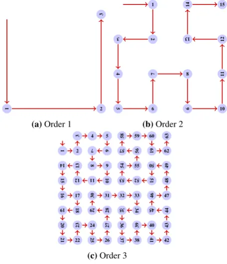
n(t0)andn(t00)members of the series. So points on the same line correspond to elements that follow one in the series but not between lines. As an example we can see on the figure 1 that the 15th node has as neighbors the 14th and 16th nodes but also the 8th and 20th node that are not close from it in the sequence.
Thus, to obtain a better representation of our series in a two-dimensional space we need another algorithm. A space filling curve is a continuous one-to-one function which map a compact interval to a multi-dimensional unit hypercube[6]. Space filling curves were discovered by the mathematician Giuseppe Peano in 1890[15]. For our purposes, we take out a
1 2 3 4 5
6 7 8 9 10 11 12
13 14 15 16 17
18 19 20 21 22 23 24
[image:2.595.362.473.63.157.2]25 26 27 28 29
Figure 1.Standard curve
specific example of such a curve, the one proposed by David Hilbert[7] shortly after Peano’s discovery.
A Hilbert Curve is a space filling curve which maps a one-dimensional interval into a two-one-dimensional area. Its con-struction is based on the repetition of a simple pattern: the first three sides of a square. At each repetition the square is turned, reduced and repeated until to obtain a curve that fills the plan. In fact, a Hilbert curve can be regarded as a Linden-mayer system[19], also known as an L-system. A L-system is a string rewriting system that can be used to generate frac-tals with dimension between 1 and 2. For the Hilbert curve the L-system rules are:
L= +RF−LF L−F R+
R=−LF+RF R+F L−
withL andR as L-system alphabet, F means draw for-ward,−means turn left 90 and+means turn right 90.
The first orders of the Hilbert curve are presented in the figure 2. As we can see on the pictures 2a, 2b and 2c, each point has an index corresponding to the index of each entry in the series. We can see that unlike our first approach described above, the use of Hilbert Curve permit us to preserve data locality, meaning that points close in the series remain close in the two-dimensional space.
1
2
3
(a)Order 1
1 2 3 4 5 6 7 8 9 10 11 12 13 14 15
(b)Order 2
1
2
3 4 5
6 7 8 9 10 11 12 13 14 15 16 17 18 19 20 21 22 23 24 25 26 27 28 29
30 31 32 33
34 35 36 37 38 39 40 41 42 43 44 45 46 47 48 49 50 51 52 53 54 55 56 57 58 59 60
61
62
63
(c)Order 3
Figure 2.First orders of Hilbert curve
[image:2.595.310.538.507.772.2]3.2
3D representation
After the two-dimensional approach, we will try to repre-sent the sequences obtained in a 3D environment.
As we have said above, a PRBG is comparable to a non-linear system generating a chronological series of data. One of the most commonly used means for analysing a series of this type is to rebuild its phase space using the method of delays [9]. The phase space is a space ofndimensions that completely describes the state of anvariables system. For example, the phase space describing the landing of a rocket is a two-dimensional space. The first dimension is the ve-locity of the rocket and the second dimension is the ground distance. The phase space is then a graph representing the velocity on x-axis and the ground distances on y-axis. Thus, for the rocket to land smoothly, it is necessary that the curve describing the progress in its phase space tends to zero (see figure 3).
Speed inkm/h
Distance to the ground inm
0 100 200 300 400
0 1000 2000 3000 4000
[image:3.595.325.534.267.437.2]Rocket progression
Figure 3.Phase space of the rocket path
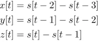
Here, our goal is to represent in three-dimensional a one-dimensional sequence. The method of delays [14] allows to reconstruct the missing dimensions using the previous values as additional coordinates. For this, instead of using the raw values returned by the function, we calculate, for each coor-dinate, the difference of two successive values. This allows us to generate more useful results to show the dynamics of the function. So ifs[t]is the sequence provided by a PRBG in function of timet, then the coordinatesx,y,zof a point in our environment are calculated from following equations:
x[t] =s[t−2]−s[t−3]
y[t] =s[t−1]−s[t−2]
z[t] =s[t]−s[t−1]
Then, representing the point sequence thus obtained in a three-dimensional environment we obtain a specific shape to the given function of PRBG. This form, calledattractor, re-veals the complex nature of the dependencies between the different elements of the sequence generated by the algorithm investigated [22, 23].
As a concrete example, the sequence of numbers of the figure 4 comes from the PRBG algorithm that generates
the TCP session sequence numbers of the operating system GNU/Linux RedHat in its version 7.3.
[image:3.595.70.286.292.497.2]3281499104, 3271545868, 3287443610, 3238749981, 3274168813, 3302234066, 3229771300, 3287970591, 3295595222, 3298841199, 3292774952, 3294591612, 3294540537, 3294046036, 3296969037, 3293746299, 3300112100, 3292483752
Figure 4.Sample sequences of Redhat 7.3 PRBG
At first glance, it is difficult to determine whether there is a link between the different elements of this sequence of numbers. By cons, the figure 5 formalizes this relationship by unveiling a shape that is characteristic of PRBG used by the Linux 2.4.18 kernel used by this Linux distribution.
Figure 5.Attractor of Redhat 7.3 PRBG - view45◦
Through this presentation mode, we are now easier to iden-tify a PRBG algorithm, given that the same algorithm will always give the same attractor.
4
PRBG samples
We will now study some PRBG algorithms.
4.1
True alea
Before starting our comparison of PRBG, we need a refer-ence, that is to say the representation of the attractor of a true alea. As a computer is a deterministic engine, it is not pos-sible to it to produce a true alea. Only hardware equipment based on physical random elements can provide this type of alea.
The websitewww.random.orgprovides the ability to gen-erate sequences of true alea. It uses atmospheric noise to produce this alea. This site is the result of a scientific project of Dr. Mads Haahr from the “School of Computer Science and Statistics” from Dublin Trinity College. It is used for online games, to generate the random lottery games, for sci-ence projects. . . We generated a sequsci-ence of 10 000 random integers from this site. The first inputs of this sequence are as presented in figure 6.
And the 3-dimensional representation of the corresponding attractor is shown in figure 7.
[image:3.595.127.230.677.720.2]72329, 95447, 11130, 52803, 25986, 58390, 84305, 98618, 54545, 64850, 27412, 15977, 13214, 30421, 91625, 48878, 35783, 58844, 16061, 74799
[image:4.595.60.267.135.310.2]Figure 6.Sample sequences of true alea
Figure 7.Attractor of a true alea - view45◦
andzin blue. The distribution of points in this space forms a homogeneous cloud and evenly covers the volume along the three axes. No specific pattern emerges. The values provided are between0and99995with an average value of54707.79. In the right corner we have the Hilbert curve representation of the data set. The colors in this curve seem completely ran-dom.
In addition, the program we use, assigns a specific color to each point: all the colors of the color palette is spread over all the points in chronological order. Thus, the first item on the list receives the first color in the palette, the second point receives the second color and so on until the last point. This principle allows us to add a fourth dimension to our graph: the time.
On our curve the color distribution seems completely ran-dom.
4.2
The PI digits
The number Pi is a mathematical constant defined by the ratio of a circle’s circumference to its diameter. Pi is com-monly approximated as 3.14159265. Being an irrational number, Pi cannot be expressed exactly as a fraction. The digits of Pi appear to be randomly distributed, however no proof of this has been discovered[21].
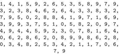
If we take the 100 first digits of Pi we obtain the sequence presented in figure 8. And the 3-dimensional representation of the corresponding attractor is shown in figure 9.
1, 4, 1, 5, 9, 2, 6, 5, 3, 5, 8, 9, 7, 9, 3, 2, 3, 8, 4, 6, 2, 6, 4, 3, 3, 8, 3, 2, 7, 9, 5, 0, 2, 8, 8, 4, 1, 9, 7, 1, 6, 9, 3, 9, 9, 3, 7, 5, 1, 0, 5, 8, 2, 0, 9, 7, 4, 9, 4, 4, 5, 9, 2, 3, 0, 7, 8, 1, 6, 4, 0, 6, 2, 8, 6, 2, 0, 8, 9, 9, 8, 6, 2, 8, 0, 3, 4, 8, 2, 5, 3, 4, 2, 1, 1, 7, 0, 6,
[image:4.595.301.514.349.512.2]7, 9
Figure 8.100 first digits of Pi
Figure 9.Attractor of the Pi digits - view45◦
In figure 9, we can see that the Hilbert curve shows a color distribution that seems random. However the 3-dimensional view shows a cloud of point close to the real random but with some ordered alignments. It appears there that the Pi digits are not truly random.
Figure 10.Attractor of the Pi digits (grouping by 4) - view45◦
In fact, this effect of ordered alignments is due to the limit of the Pi digits. Indeed, they are between 0 and 9 and the various possible combinations of these decimals in the sub-tractions which we make to calculate the coordinatesx,y, andz are limited. By grouping them by 4, we obtain one distribution of the results which stages between 0 and 9999. The obtained result is more relevant. The figure 10 she shows then a perfectly random cloud. We thus have a first approach of the confirmation of the hypothesis of the alea of the digits of the Pi number.
4.3
Linear congruence generator
The linear congruence generator produces a pseudo-random sequence of integersx1, x2,x3. . . according to the
following linear recurrence [12, 10]:
xn+1=axn+b (mod m) | n≥0
The integersa,bandmare the parameters that character-ize the generator andx0is the seed. An example of generated
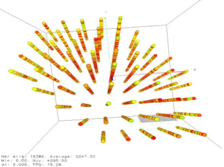
sequence witha= 5,b= 3andm= 4096is given below : The attractor for thexn+1 = 5xn+ 3 (mod 4096)
[image:4.595.67.260.703.791.2]772, 3863, 2934, 2385, 3736, 2299, 3306, 149, 748, 3743, 2334, 3481, 1024, 1027, 1042, 1117, 1492, 3367,
454, 2273, 3176, 3595, 1594, 3877, 3004, 2735, 1390, 2857, 2000, 1811,
866, 237, 1188, 1847, 1046, 1137
[image:5.595.64.268.174.332.2]Figure 11.Sample sequences of linear congruence generator
Figure 12.Attractor of the linear congruence generator - axey→y0
The sample size is16384, the minimum is0and the max-imum4095the average value is2047.50.
The color distribution in the Hilbert curve seems random. But, unlike true random generator that we have taken as a reference, the distribution of points in figures 12 and 13 has a specific pattern in the form of lines aligned on several levels. These lines correspond to the period of the algorithm.
Finally, we note that only the red predominantly colors ap-pear, it means that only the end of the spectrum is visible. The first points are covered by the latest, the algorithm therefore provides several times the same values.
[image:5.595.324.523.333.492.2]This type of generator is predictable and is not suitable for cryptographic use. Indeed, from a partial sequence, and with-out knowledge of the parametersa,bandm, it is possible to reconstruct the rest of the sequence. Moreover, in this case, the both representation – in two and three-dimensional – per-mit us to refine the randomness property of this algorithm.
Figure 13.Attractor of the linear congruence generator - axez→z0
4.4
Nonlinear recurrence generator
For our next example, we use a nonlinear recurrence gen-erator. The latter produces a pseudorandom sequence of in-tegersx1,x2,x3. . . according to the following recurrence
re-lation [20]:
xn+1=λxn(1−xn) | n≥0
This suite called “logistic” leads, if λ > 3,56995, to a chaotic suite. Logistic suite is used to model the size of a biological population over generations [11]. An example of generated sequence is given below:
451098855224, 451068728783, 451038599037, 451008465983, 450978329622, 450948189954, 450918046977, 450887900692, 450857751097, 450827598193, 450797441977, 450767282451,
The attractor for this function with the following variables
λ= 3.8andx0= 0.7364738523is given in figure 14.
Figure 14.Attractor of the nonlinear recurrence generator - axey→y0
The figure 14 also shows a specific pattern that makes it an unsafe PRBG for cryptographic application. However, unlike the linear congruence generator, we have no more appearance of periodic pattern. The generated data are not random in the first iterations (green color) then appear to become more random so with the increase of the number of iterations.
In this case, studying the Hilbert curve is interesting be-cause the color distribution seems random at the beginning but becomes quickly uniform at the end of the list (same color).
In our example, the sample size is 16384, the min-imum is 184264892666.96 and the maximum value 948850856936.47sample average is631015962902.33.
4.5
Blum-Blum-Shub generator
The pseudorandom bit generator Blum-Blum-Shub is a computationally secure PRBG as factoring large prime num-bers remains insoluble. This generator produces a pseudo-random bit sequence in accordance with the following algo-rithm:
[image:5.595.59.281.635.801.2]• choose a seed s in the range [1, n − 1] such that gcd(s, n) = 1;
• computex0=s2 (mod n);
• the sequence is defined asxi+1=x2i (mod n);
• ifxiis even thenzn = 0and ifxnis odd thenzn = 1;
• the output of the sequence isz1,z2,z3,. . .
[image:6.595.305.491.313.463.2]The attractor of this function is shown in figure 15. To facilitate the implementation of our presentation, we did not apply the final step of recovering the least significant bit. Fi-nally, we note that the attractor obtained is spread over the three axes in the form of a homogeneous cloud. We find the same form as in the case of the true alea. Actually, the Blum-Blum-Generator is cryptographically secure assuming the intractability of the quadratic residuosity problem [1]. In our example, the sample size is16384, the minimum is 56782881.0and the maximum value is512462853845.0, the sample average is257668663192.64.
Figure 15.Attractor for the Blum-Blum-Shub generator - view45◦
5
Cryptographic algorithms
5.1
RC4 attractor
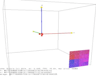
To calculate the attractor of the RC4 algorithm, we start from the sequence of integers n = 2105 + i with i =
[1· · ·60 000]that we convert in 128-bit blocks. We then en-crypt each block with the same enen-cryption 64-bit key:
k=0101010101010101 (1)
Finally, we convert the result to integers. So we start from a linear sequence of integers to get a pseudorandom sequence of integers. The following list shows the result for the first 8 entries in the sequence:
RC4k(2105+ 1) =16 (06080c0e182029293933495766768782)
=10 (8017150855153813117600873193181448066)
RC4k(2105+ 2) =16 (06080c0e182029293933495766768781)
=10 (8017150855153813117600873193181448065)
RC4k(2105+ 3) =16 (06080c0e182029293933495766768780)
=10 (8017150855153813117600873193181448064)
RC4k(2105+ 4) =16 (06080c0e182029293933495766768787)
=10 (8017150855153813117600873193181448071)
RC4k(2105+ 5) =16 (06080c0e182029293933495766768786)
=10 (8017150855153813117600873193181448070)
RC4k(2105+ 6) =16 (06080c0e182029293933495766768785)
=10 (8017150855153813117600873193181448069)
RC4k(2105+ 7) =16 (06080c0e182029293933495766768784)
=10 (8017150855153813117600873193181448068)
RC4k(2105+ 8) =16 (06080c0e18202929393349576676878b)
=10 (8017150855153813117600873193181448075)
We developed a suite of specific tools (see Appendix A.2) to generate the list and then display it in a three dimensional environment like the approach outlined above for PRBG. We get the figure 16.
Figure 16.RC4 attractor - axex→x0
The attractor of RC4 is very sparse and boils down to three red balls. The color is important, it is the color of the end of the panel color. So we can deduce that all points of the attractor have the same coordinates. We are far from a ran-dom distribution of the space like with the Blum-Blum-Shub generator.
If we change the key we obtain different kinds of attractor: figure 17 and figure 18. So we have a close link between the obtained attractor and the key used. The Hilbert curve repre-sentation of RC4 shows the same link between the attractor and the key used but more important it shows that this algo-rithm does not seems really close to the perfect randomness.
5.2
Enigma machine attractor
The Enigma machine was invented by German engineer Arthur Scherbius in 1927 [8]. The Model A was quickly abandoned in favor of the model B, of the size of a type-writer then by a portable version equipped with lamps indi-cators with the model C. The Enigma machine and the com-pany Scherbius founded for marketing, will vegetate during the inter-war. The Wehrmacht buys some copies for evalua-tion. Its only when Hitler began to rearm Germany than the cryptology experts of the Wehrmacht decide to adopt it and to equip the German army.
[image:6.595.48.239.389.530.2]Figure 17.RC4 attractor -k=5555555555555555- axex→x0
Figure 18.RC4 attractor -k=0f0f0f0f0f0f0f0f- axex→x0
the R2 rotor rotates according to the movement of the R3
that acts like an odometer. The movement of the rotor gener-ates a different combination each time a key is pressed. The encryption key is defined by the initial position of the three rotors.
To calculate the attractor of the Enigma machine, we use a sequence comprising all possible combinations of 5 char-acters from AAAAA to EZZZZ. That is to say 5 ×264 =
2284880 inputs. Each of them is then encrypted using a program reproducing operation of a three rotors Enigma ma-chine. The used key isAAA. The obtained result is then con-verted to hexadecimal. Thus the sequenceAAAAAbecomes
FTZMG ⇒ (0x46545a4d47) and EZZZZ becomes DXILI
⇒ (0x4458494c49).
The attractor of the Enigma machine in a 3-Dimensions world is presented in the figure 19 page 177.
The analysis of the attractor of the Enigma shows a cloud of random points. However, we distinguish alignments and a cloud of scattered enough points. Since there are more than two million points we should have a denser cloud.
By zooming in the graph (figure 20 page 177), we are see-ing that points are grouped in clusters and there colors are similar. By counting the points inside clusters we find they contains approximately 26 points, ie a point for each charac-ter of alphabet. We have no explanation for this fact, it needs more investigations.
5.3
AES attractor
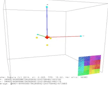
To calculate the attractor of the AES, we start from the sequence of integersn= 2105+iwithi= [1· · ·1 000 000]
[image:7.595.65.251.248.394.2]that we convert in 128-bit blocks. We then encrypt each block
Figure 19.Enigma machine attractor - view45◦
Figure 20.Enigma machine attractor - zoomed view
with the same encryption key:
k=80000000000000000000000000000000 (2)
Finally, we convert the result to integers. So we start from a linear sequence of integers to get a pseudorandom sequence of integers. The following list shows the result for the first 8 entries in the sequence:
AESk(2105+ 1) =16 (d557cc9f49fe887227b4b9ddece84715)
=10 (283581443160616712863761136161128990485)
AESk(2105+ 2) =16 (09c7c5a6ebf426a5f19e03bd9040e79d)
=10 (13000327896503708020216929648547784605)
AESk(2105+ 3) =16 (5f8fc8bf51275ac26522097cb3035f0b)
=10 (127023229689953121336747928769328799499)
AESk(2105+ 4) =16 (c966ecf33d34f92dc353498769996462)
=10 (267709247352391222087383818398701544546)
AESk(2105+ 5) =16 (09d800a81f3caa9871aa6ee1ee32ed4e)
=10 (13084601403506444488341809178476735822)
AESk(2105+ 6) =16 (723e5071689e7a932405c6d351a87eed)
=10 (151855545502638255213403946355100516077)
AESk(2105+ 7) =16 (56cfe7cf8cc63cbc4a527ae09957a949)
=10 (115393114767635113880023375849033541961)
AESk(2105+ 8) =16 (f7ca0f9ad9dfc972e5890cab472d3476)
=10 (329368475429008126664105441219366958198)
[image:7.595.310.536.261.435.2]Instead of the Blum-Blum-Shub generator we find that the attractor of AES takes the form of a cloud of points dis-tributed over the three axes under the form of cubes. It dif-fers, in this, from the attractor of the true alea. Nevertheless we can reasonably infer that the AES is an encryption algo-rithm designed as a pseudorandom bit generator close to the true hazard.
[image:8.595.63.247.167.306.2]Figure 21.AES attractor - axex→x0
Figure 22.AES attractor - viewz→z0
After graphically analysed the behaviour of the AES, we will try to see how the algorithm behaves with different en-cryption keys. For this, we have reproduced the process de-scribed above using the same initial sequence and encrypting it with the two keys:
k1=80000000000000000000000000000000 (3)
k2=40000000000000000000000000000000 (4)
These two keys differ only on1bit over the 128 bits com-posing them.
Then assigning a different color to each attractor, we can compare them two by two. The result is shown in figures 23 and 24. To generate these figures we calculated the encryp-tion of a sequence of450000identical blocks.
[image:8.595.305.501.268.429.2]By performing the comparison of these two attractors, we find that they fit together tightly by uniformly covering the three dimensions. However, it is not possible to distinguish a possible correlation between these two sets of elements. To help visualize a possible correlation between the two sets
[image:8.595.61.245.374.533.2]Figure 23.Attractors of two AES ciphers with different keys - axex→x0
Figure 24.Attractors of two AES ciphers with different keys - viewz→z0
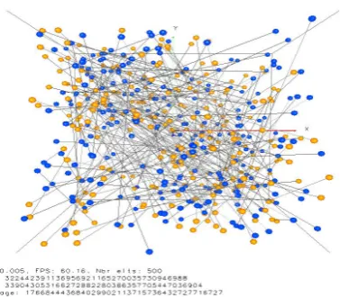
of encrypted blocks, we will represent the same graph but by joining two by two the corresponding points of the same input. Thus, the point representing the encrypted block with the keyk1of the first block of the sequence will be linked to
the corresponding point in the encrypted block with the key
k2of the same block in the clear.
The result is shown in figures 25 and 26. In the aims that the graphs are readable, we have reduced the size of the sam-ple to255entries. The straight path connecting the points is messy and shows no identifiable pattern.
Figure 25.Correlation between two AES attractors - view45◦
[image:8.595.313.514.609.766.2]Figure 26.Correlation between two AES attractors - axez→z0
encryption keys. Calculating Minkowski distances [18] with
p= 2for each point of the graph confirms this result. Indeed, the list of distances, whose first inputs are shown below, be-have as a random sequence. The attractor arising from the representation of these distances in three dimensions (see fig-ure 27) has the form of a cloud whose specific form is close to that a diamond. It would be interesting to try to understand what justifies this form, but it is not the subject of this work.
12026847709294981120, 12026869209288865792, 19971070890283577344, 26113153353646714880, 25972774069680922624, 14954846745435789312, 7391670208430327808, 1673631091276342528, 2444035869612603904, 2802878496097698304, 2426843600751804928, 1753123651095763712, 9810861268161230848, 10326031878050832384, 16430236778313869312, 14585735298828013568,
14873569053264308224, 13174990125624895488
Figure 27.Attractor of distances between two encryption process with the AES - view45◦
6
Conclusion
Our analysis of the hazard produced by PRBG and in par-ticular by the cryptographic algorithms, although visually speaking, is not sufficient to prove that the sequences pro-duced by its algorithms are statistically random.
However, viewing of the hazard, as we have shown, has two attractive advantages: the first is that it can detect
pat-terns and thus here some problems since we are seeking ran-domness, and second is the fact that our brain has more abil-ity to quickly distinguish two different pictures, our approach allows us to more easily recognize and differentiate PRBG from another. Thus, just by displaying in environments in two and three dimensions the output of a random sequences, we have the opportunity to detect possible patterns and iden-tify the PRBG used to generate the sequence. This approach also allows us to realize a first and quick analysis of potential biases on unknown cryptographic algorithms.
We developed some tools that offer the opportunities to apply our approach on some PRBG and cryptographic algo-rithms. Our aim is to implement more and more of these al-gorithms to construct a database of attractors that can be used to attribute the proper PRBG or cryptographic algorithm to a random number sequence.
Acknowledgements
The authors wish to thank Alexey Zhukov of the Bauman Moscow State Technical University for his valuable com-ments to this research work.
A
Listings of programs
The entire program code developed during this article is available on GitHub (https://github.com/archoad). These programs are all under GPL v3.
A.1
PRBG generating and viewing in 3D
Available at the linkhttps://github.com/archoad/PRBG-3D. To run this suite of programs requires a C compiler and OpenSSL and OpenGL libraries.
A.2
Encryption algorithms and 3D
visualiza-tion
Available at the linkhttps://github.com/archoad/VisCipher3d.
To run this suite of programs requires a C compiler and the OpenSSL libraries (using the libcrypto for encryption and the BIGNUM API) and OpenGL.
REFERENCES
[1] L. Blum, M. Blum, and M. Shub. Comparison of two pseudo-random number generators.Advances in Cryp-tology, 82:61–78, 1983.
[2] G. Conti and S. Bratus. Voyage of the reverser: A visual study of binary species.Black Hat USA, 2010.
[3] G. Conti, E. Dean, M. Sinda, and B. Sangster. Visual reverse engineering of binary and data files. Workshop on Visualization for Computer Security (VizSEC), 2008. [4] C. Domas. The future of re: Dynamic binary
visualiza-tion.Reverse engineering conference (REcon), 2013. [5] E. Filiol. A new statistical testing for symmetric ciphers
and hash functions. Proceedings of Information and
[image:9.595.70.273.493.664.2][6] C. Hamilton. Compact hilbert indices.Technical report
CS-2006-07, 2006.
[7] D. Hilbert. Ueber die stetige abbildung einer line auf ein flchenstck. Mathematische Annalen, 38:459–460, 1891. http://dx.doi.org/10.1007/BF01199431.
[8] D. Kahn. The Codebreakers. Scribner, 1996.
[9] M. Kennel, R. Brown, and H. Abarbanel. Determin-ing embeddDetermin-ing dimension for phase-space reconstruc-tion using a geometrical construcreconstruc-tion. Phys. Rev. A, 45:3403–3411, 1992.
[10] D. E. Knuth. The Art of Computer Programming, vol-ume Volvol-ume 2 - Seminvol-umerical Algorithms. Addison Wesley, 1981.
[11] R. May. Simple mathematical models with very complicated dynamics. Nature, 261:459–467, 1976. http://abel.harvard.edu/archive/118r-spring-05/docs/may.pdf.
[12] A. Menezes, P. Oorschot, and S. Vanstone. Handbook of applied cryptography. CRC Press, 1997.
[13] K. Nance, S. Tricaud, and P. Saad. Visualizing network activity using parallel coordinates. 44th Hawaii Inter-national Conference on System Sciences, 2011. [14] N. Packard, J. Crutchfield, D. Farmer, and R. Shaw.
Ge-ometry from a time series. Physical Review Letters, 45:712–716, 1980.
[15] G. Peano. Sur une courbe, qui remplit toute une aire plane. Mathematische Annalen, 36:157–160, 1890. http://dx.doi.org/10.1007/BF01199438.
[16] S. Tricaud and P. Saad. Applied parallel coordinates for logs and network traffic attack analysis. Journal in Computer Virology, 6:1–29, 2010.
[17] J. von Neumann. Various techniques used in connection with random digits. Monte Carlo Method, 12:36–38, 1951.
[18] E. Weisstein. Distance, 2014.
http://mathworld.wolfram.com/Distance.html.
[19] E. Weisstein. Hilbert curve, 2014. http://mathworld.wolfram.com/HilbertCurve.html. [20] E. Weisstein. Logistic map, 2014.
http://mathworld.wolfram.com/LogisticMap.html.
[21] E. Weisstein. Pi digits, 2014.
http://mathworld.wolfram.com/PiDigits.html.
[22] M. Zalewski. Strange attractors and tcp/ip se-quence number analysis. lcamtuf.coredump.cx, 2001. http://lcamtuf.coredump.cx/oldtcp/tcpseq.html. [23] M. Zalewski. Strange attractors and tcp/ip sequence