Implicit Two point Block Method with Third and Fourth Derivatives for Solving General Second Order ODEs

Implicit Two-point Block Method with Third and Fourth

Derivatives for Solving General Second Order ODEs

Reem Allogmany

1,2,∗

_,

_{Fudziah Ismail}

1,3

_,

_{Zarina Bibi Ibrahim}

1,3

1 _{DepartmentofMathematics,FacultyofScience,UniversitiPutraMalaysia,43400UPM,Serdang,Selangor,Malaysia}

2_{DepartmentofMathematics,TaibahUniversity,Al-Medina,SaudiArabia}

3_{InstituteforMathematicalResearch,UniversitiPutraMalaysia,43400UPM,Serdang,Selangor,Malaysia}

Copyright c2019 by authors, all rights reserved. Authors agree that this article remains permanently open access under the terms of the Creative Commons Attribution License 4.0 International License

Abstract

In this paper we present an implicit two-point block method for solving directly the general second order ordinarydifferentialequations(ODEs). Themethod incorpo-ratesthefirsta nds econdd erivativeso ff(x,y,y0),w hichare thethirdandfourthderivativesofthesolution. Themethodis derived using Hermite Interpolating Polynomialas the basic function. Aperformancecomparisonof the two-pointblock method is compared interm of accuracyto several existing methods,whichhaveorderalmostequalorhigherthanthatof thenewmethod. Numericalresultsinterprettheaccuracyand efficacyofthenewm ethod.Applicationofthenewmethodis discussed.

Keywords

Implicit, BlockMethod, SecondOrderODEs, HermiteInterpolation

1

Introduction

The second order ordinary differential equations arise in many areas of applied science and engineering represented by mathematical models. Commonly, second order ODEs can be solved by reducing the equation into system of first order ODEs, but this could be computationally costlier than the direct methods. Some attention by some eminent scholars has been given to solve the problem directly, such as [1]- [4]. How-ever, Awoyemi [5], Akinfenwa and Jator [6]developed meth-ods of higher order ODEs directly. The techniques for solving the problem directly are (i) using interpolation and collocation technique, which is the most common, see [7]- [10], and (ii) using interpolation and integration technique. Several studies have been conducted to implement derivative methods in solv-ing ODEs, see [11]- [16].

In this paper, we develop a two-point block implicit method by using interpolation and integration technique, which involved the third and fourth derivatives of the solution in (1) with a constant step-size, which aim at obtaining more accurate nu-merical results. We are concerned with development of the numerical solution of initial value problems (IVPs) for

second-order ODEs of the form:

y00=f(x, y, y0) y(a) =y0 y0(a) =y00 x∈[a, b]

(1) where the third and fourth derivatives of the solution to (1) are

y000 = f0(x, y, y0) =fx+fyy0+fy0f =g(x, y, y0),

and

y(4) = f00(x, y, y0) =fxx+fxyy0+fxy0f + (f_xy

+ fyyy0+fyy0f)y0+f_yf =q(x, y, y0),

2

Derivation of the Method

The derivation of the proposed method is based on Hermite Interpolating PolynomialP2(x),which interpolatesf(x, y, y0)

at two-points. The polynomial has the form

P(x) =

n

X

i=0

mi−1

X

k=0

f_i(k)Li,k(x) (2)

where,

fi=f(xi, yi, yi0), xi=a+ih, i= 0,1, ..., n

h=b−a

n ,

L(i,k)(x)is the generalized Lagrange polynomial

i = 0,1, ..., n, k = 0,1, ..., mi andnis a positive integer.

In order to compute the two approximation values ofyn+1and

yn+2simultaneously atxn+1andxn+2, wherexnbecomes the

starting point andxn+2is the last point in the block with step

size 2h. The evaluation solution of yn+2 at the point xn+2

[image:2.595.305.553.88.326.2]

Figure 1.Two point block method.

two points at each block as shown in the Figure 1. The method will compute two points concurrently using one earlier block.

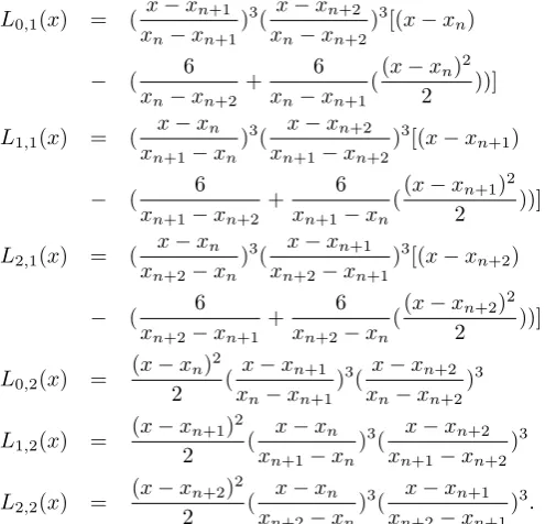
P2(x) = L0,0(x)f0+L1,0(x)f1+L2,0(x)f2+L0,1(x)g0

+ L1,1(x)g1+L2,1(x)g2+L0,2(x)q0+L1,2(x)q1

+ L2,2(x)q2

Wheregandqare the third and fourth derivatives of the solu-tion respectively and

L0,0(x) = (

x−xn+1

xn−xn+1

)3( x−xn+2

xn−xn+2

)3[1−( 3

xn−xn+1

+ 3

xn−xn+2

)((x−xn)−

(x−xn)2

2 (

6

xn−xn+2

+ 6

xn−xn+1

))−( 6 (xn−xn+1)2

+ 6

(xn−xn+2)2

+ 18

(xn−xn+1)(xn−xn+2)

)((x−xn)

2

2 )]

L1,0(x) = (

x−xn

xn+1−xn

)3( x−xn+2

xn−xn+2

)3[1−( 3

xn+1−xn+2

+ 3

xn+1−xn

)((x−xn+1)

− (x−xn+1)

2

2 (

6

xn+1−xn+2

+ 6

xn+1−xn

))

− ( 6

(xn+1−xn+2)2

+ 6

(xn+1−xn)2

+ 18

(xn+1−xn)(xn+1−xn+2)

)(x−xn+1)

2

2 ]

L2,0(x) = (

x−xn

xn+2−xn

)3( x−xn+1

xn+2−xn+1

)3[1

− ( 3

xn+2−xn

+ 3

xn+2−xn+1

)((x−xn+2)

− (x−xn+2)

2

2 (

6

xn+2xn+1

+ 6

xn+2−xn

))

− ( 6

(xn+2−xn+1)2

+ 6

(xn+2−xn)2

+ 18

(xn+2−xn)(xn+2−xn+1)

)((x−xn+2)

2

2 )]

L0,1(x) = (

x−xn+1

xn−xn+1

)3( x−xn+2

xn−xn+2

)3[(x−xn)

− ( 6

xn−xn+2

+ 6

xn−xn+1

((x−xn)

2

2 ))]

L1,1(x) = (

x−xn

xn+1−xn

)3( x−xn+2

xn+1−xn+2

)3[(x−xn+1)

− ( 6

xn+1−xn+2

+ 6

xn+1−xn

((x−xn+1)

2

2 ))]

L2,1(x) = (

x−xn

xn+2−xn

)3( x−xn+1

xn+2−xn+1

)3[(x−xn+2)

− ( 6

xn+2−xn+1

+ 6

xn+2−xn

((x−xn+2)

2

2 ))]

L0,2(x) =

(x−xn)2

2 (

x−xn+1

xn−xn+1

)3(x−xn+2

xn−xn+2

)3

L1,2(x) =

(x−xn+1)2

2 (

x−xn

xn+1−xn

)3( x−xn+2

xn+1−xn+2

)3

L2,2(x) =

(x−xn+2)2

2 (

x−xn

xn+2−xn

)3( x−xn+1

xn+2−xn+1

)3.

The approximation values ofyn+1andyn+2at the pointsxn+1

andxn+2can be obtained by:

First point: integrating (1) once and twice with respect tox

over the interval[xn, xn+1]. The following formulae can be

obtained

Z xn+1

xn

y00dx=

Z xn+1

xn

f(x, y, y0)dx (3)

Z xn+1

xn

Z x

xn

y00dxdx=

Z xn+1

xn

Z x

xn

f(x, y, y0)dxdx (4)

Letxn+1=xn+hwhich gives

y0(xn+1) =y0(xn) +

Z xn+1

xn

f(x, y, y0)dx (5)

y(xn+1) =y(xn) +hy0(xn) +

Z xn+1

xn

(xn+1−x)f(x, y, y0)dx

(6) Then,f(x, y, y0)in (5) and (6) will be replaced with Hermite Interpolating PolynomialP2(x).

By takingx=xn+2+shands= x−xn_h+2 anddx=hds

and changing the limit of integration from−2to−1, we have

y0(xn+1) = y0(xn) +

Z −1

−2

[f0L0,0(s) +f1L1,0(s) +f2L2,0(s)

+ g0L0,1(s) +g1L1,1(s) +g2L2,1(s) +q0L0,2(s)

+ q1L1,2(s) +q2L2,2(s)]hds (7)

y(xn+1) = y(xn) +hy0(xn) +

Z −1

−2

[f0L0,0(s) +f1L1,0(s)

+ f2L2,0(s) +g0L0,1(s) +g1L1,1(s) +g2L2,1(s)

where,

L0,0 =

1 16(s+ 1)

3_s3_(24s2_{+ 105s+ 116)}

L1,0 = −(2 +s)3s3(3s2+ 6s+ 4)

L2,0 =

1

16(2 +s)

3_{(s+ 1)}3_(24s2_{−9s+ 2)}

L0,1 =

h

8(2 +s)(s+ 1)

3_s3_{(10 +}9

2s)

L1,1 = −h(s+ 1)(2 +s)3s3

L2,1 =

−9

16hs(s+ 1)

3_{(2 +s)}3₍−2

9 +s)

L0,2 =

h2

16(s+ 1)

3_{(2 +s)}2_s3

L1,2 =

−h2

16 (s+ 1)

3_{(2 +s)}2_s3

L2,2 =

h2

16(s+ 1)

3_{(2 +s)}3_s2

Evaluating the integrals in (7) and (8) usingMAPLE, gives,

y0_n+1 = y_n0 + h

13440(5669fn+ 8192fn+1−421fn+2)

+ h

2

4480(303gn−560gn+1+ 47gn+2) (9)

+ h

3

40320(169qn+ 1024qn+1−41qn+2)

yn+1 = yn+hyn0 +

h2

60(19fn+ 12fn+1−fn+2)

+ h

3

20160(911gn−1024gn+1+ 113gn+2) (10)

+ h

4

20160(53qn+ 252qn+1−11qn+2)

Similarly,

Second point:integrating (1) once and twice with respect tox

over the interval[xn+1, xn+2]. The following formulae can be

obtained

Z xn+2

xn+1

y00dx=

Z xn+2

xn+1

f(x, y, y0)dx (11)

Z xn+2

xn+1

Z x

xn+1

y00dxdx=

Z xn+2

xn+1

Z x

xn+1

f(x, y, y0)dxdx (12)

Letxn+2=xn+1+hwhich gives

y0(xn+2) =y0(xn+1) +

Z xn+2

xn+1

f(x, y, y0)dx (13)

y(xn+2) =y(xn+1)+hy0(xn+1)+

Z xn+2

xn+1

(xn+2−x)f(x, y, y0)dx

(14) Then,f(x, y, y0)in (13) and (14) will be replaced with Hermite Interpolating PolynomialP2(x).

By takingx=xn+2+shands=

x−xn+2

h anddx=hds

and changing the limit of integration from−1to0, we have

y0(xn+2) = y0(xn+1) +

Z 0

−1

[f0L0,0(s) +f1L1,0(s)

+ f2L2,0(s) +g0L0,1(s) +g1L1,1(s) +g2L2,1(s)

+ q0L0,2(s) +q1L1,2(s) +q2L2,2(s)]hds (15)

y(xn+2) = y(xn+1) +hy0(xn+1)

+

Z 0

−1

[f0L0,0(s) +f1L1,0(s) +f2L2,0(s)

+ g0L0,1(s) +g1L1,1(s) +g2L2,1(s) (16)

+ q0L0,2(s) +q1L1,2(s) +q2L2,2(s)]hds

Evaluating th integrals in (15) and (16) usingMAPLE, gives,

yn0+2 = yn0+1+

h

13440(−421fn+ 8192fn+1+ 5669fn+2)

+ h

2

4480(−47gn+ 560gn+1−303gn+2) (17)

+ h

3

40320(−41qn+ 1024qn+1+ 169qn+2)

yn+2 = yn+1+hy0n+1+

h2

13440(−197fn+ 5504fn+1 + 1413fn+2) +

h3

40320(−197gn+ 2992gn+1 (18) + 905gn+2) +

h4

40320(−19qn+ 520qn+1+ 63qn+2)

The formulae (9),(10),(17) and(18) can be written in a matrix difference equation to obtain the order of the new method as follows :

αYm=hβYm0 +h

2_γF

m+h3δGm+h4ζQm,

whereβ, γ, δ, andζdefined as,

α=



  

0 0 0 0

0 −1 1 0

0 0 0 0

0 0 −1 1



  

, β=



  

0 1 −1 0 0 1 0 0 0 0 1 −1 0 0 1 0

    , γ=    

0 ₁₃₄₄₀5669 ₁₀₅64 ₁₃₄₄₀−421 0 19₆₀ 1₅ −₆₀1 0 ₁₃₄₄₀−421 ₁₀₅64 ₁₃₄₄₀5669 0 ₁₃₄₄₀−197 ₁₀₅43 ₄₄₈₀471



  

, δ=



  

0 ₄₄₈₀303 −₈1 ₄₄₈₀47 0 ₂₀₁₆₀911 −₃₁₅16 ₂₀₁₆₀113 0 ₄₄₈₀−47 1₈ −₄₄₈₀303 0 ₄₀₃₂₀−197 ₂₅₂₀187 −₈₀₆₄181

    , ζ=    

0 ₄₀₃₂₀169 ₃₁₅8 ₄₀₃₂₀−41 0 ₂₀₁₆₀53 ₈₀1 ₂₀₁₆₀−11 0 ₄₀₃₂₀−41 ₃₁₅8 ₄₀₃₂₀169 0 ₄₀₃₂₀−19 ₁₀₀₈13 ₆₄₀1



  

, , Ym=



  

yn−1

yn

yn+1

yn+2



  

,

Y_m0 =



  

y0_n−1 y0_n y0_n+1 y0_n+2



  

, Fm=



  

fn−1

fn

fn+1

fn+2

    ,    

gn−1

gn

gn+1

gn+2



  

, Qm=



  

qn−1

qn

qn+1

qn+2



  

.

According to Henrici[16], it can be said that the new methods haveorder pifC0=C1 =Cp = 0 =Cp+1 = 0,Cp+26= 0,

which is the error cosntant. Where

C0=

k

X

j=0

αj C1=

k

X

j=0

C2= k X j=0 (j 2

2!αj−βj),

C3=

k

X

j=0

(j

3

3!αj−jβj−γj),

.. .

Cq = k

X

j=0

jq q!αj−

K

X

j=0

jq−1

(q−1)!βj−

K

X

j=0

jq−2

(q−2)!γj, q= 4,5, ..

In our method C0 = C1 = ...C9 = 0 and C10 =

[−0.010194415,0,−0.048511786,0]TThus, we conclude that the method in(9),(10),(17)and(18) is of the order 8.

3

Implementation

In this section, we briefly mentioned the implementation of two-point block method. The approximation solutions in (9),(10),(17) and(18) will be estimated using the predictor-corrector schemes. The predictor equations using Taylor method:

y_n0p_+i = y_n0p_+(i−1)+hf_nc_+(i−1) yp_n+i = y_np_+(i−1)+hy_n0p_+(i−1)+h

2

2!f

c

n+(i−1); i= 1,2 f_np_+i(x,y,y0) = f(xn+i, ynp+i, y

0p

n+i), (19)

g_np_+i(x,y,y0) = f0(xn+i, ypn+i, y 0p n+i),

q_np_+i(x,y,y0) = f00(xn+i, y p n+i, y

0p n+i)

Define Eq.(19) as the initial approximation and applying the derived method in (9),(10),(17) and(18) as corrector. In order to obtain the corrector iteration, the following equations will

be used

y_n0c₊₁ = y_n0c+ h

13440(5669f

c

n+ 8192f p

n+1−421f

p

n+2)

+ h

2

4480(303g

c

n−560g

p

n+1+ 47g

p

n+2)

+ h

3

40320(169q

c

n+ 1024q p

n+1−41q

p n+2)

y_nc₊₁ = y_nc +hy0_nc+h

2

60(19f

c

n+ 12f

p

n+1−f

p

n+2)

+ h

3

20160(911g

c

n−1024g

p

n+1+ 113g

p n+2)

+ h

4

20160(53q

c n+ 252q

p

n+1−11q

p

n+2) (20)

y_n0c₊₂ = y_n0c₊₁+ h

13440(−421f

c

n+ 8192f p

n+1+ 5669f

p n+2)

+ h

2

4480(−47g

c

n+ 560g p

n+1−303g

p n+2)

+ h

3

40320(−41q

c

n+ 1024q p

n+1+ 169q

p

n+2)

ync+2 = y

c

n+1+hy0

c

n+1+

h2

13440(−197f

c

n+ 5504f p

n+1

+ 1413f_np₊₂) + h

3

40320(−197g

c

n+ 2992g p

n+1

+ 905g_np₊₂) + h

4

40320(−19q

c

n+ 520q p

n+1+ 63q

p

n+2)

Then, the next corrector iteration will be

y0_nc₊₁ = y_n0c+ h

13440(5669f

c

n+ 8192f p

n+1−421f

p n+2)

+ h

2

4480(303g

c

n−560g

p

n+1+ 47g

p n+2)

+ h

3

40320(169q

c

n+ 1024q p

n+1−41q

p n+2)

y_nc₊₁ = y_nc +hy_n0c+h

2

60(19f

c

n+ 12f

p

n+1−f

p n+2)

+ h

3

20160(911g

c

n−1024g

p

n+1+ 113g

p

n+2) (21)

+ h

4

20160(53q

c n+ 252q

p

n+1−11q

p n+2)

y_n0c₊₂ = y_n0c₊₁+ h

13440(−421f

c

n+ 8192f c

n+1

+ 5669f_np₊₂) + h

2

4480(−47g

c

n+ 560gnc+1

− 303g_np₊₂) + h

3

40320(−41q

c

n+ 1024q c

n+1

+ 169qp_n+2)

ycn+2 = ync+1+hy0nc+1+

h2

13440(−197f

c n

+ 5504f_nc₊₁+ 1413f_np₊₂) + h

3

40320(−197g

c n

+ 2992gc_n+1+ 905gp_n+2)

+ h

4

40320(−197q

c n+ 520q

c

n+1+ 63q

4

Problem tested

We present in this section numerical results for some tested problems and application by applying the proposed method derived in this paper usingC languagecode. The following notations will be used in the tables

I2PBDO8 The implicit two-point block method proposed in this paper, order 8. Jator1 Three step hybrid linear multistep

method with three off-step points[17], order 7.

Vigo-Ramos variable-step Falkner method in the predictor-corrector mode [18] , order 8. Jator2 The two step block hybrid third

derivative method with one off-step point [19], order 8.

Akinfenwa Four step block hybrid collocation method with four off-step points [20], order 9.

Badmus1 implicit linear multistep Hybrid Block method of Uniform order 8 at k=5 [21], order 8.

Badmus2 Uniform order eight implicit block method[22], order 8.

h step size

NS Total number of steps MAXE Maximum absolute error

4.1

problems

Proplem 1:Bessel’s differential equation:

x2_y00_+xy0_{+ (x}2_{−0.25)y= 0 [1,8]}

y(1) =

q

2

πsin(1),

y0_{(1) =} 2cos(1)−sin(1)

√

2π ,

Exact solution:

y(x) =q_πx2sin(x)

Source: Jator, S. N. (2010)

Proplem 2:A nonlinear problem

y00= 6y2_{, [0,10]}

y(0) = 1, y0(0) =−2

Exact solution:

y(x) = (1 +x)−2

Source: Singh, G., & Ramos, H. (2019)

Proplem 3:A nonlinear problem

y00+_x6y0+_x42y= 0 x >0

y(1) = 1, y0(1) = 1

Exact solution:

y(x) = 5 3x−

2 3x4

Source: Badmus, A. M. (2014b)

Proplem 4:A linear problem

y00−3y0= 8e2x, y(0) = 1, y0(0) = 1

Exact solution:

y(x) =−4e2x_{+ 3e}3x_{+ 2}

[image:5.595.331.523.395.591.2]

Source: Badmus, A. M. (2014b)

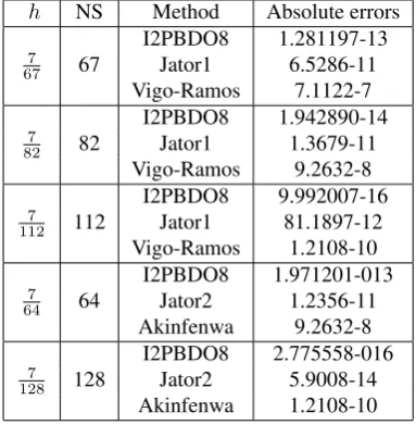
Table 1.Numerical results for solving Problem1.

h NS Method Absolute errors I2PBDO8 1.281197-13

7

67 67 Jator1 6.5286-11

Vigo-Ramos 7.1122-7 I2PBDO8 1.942890-14

7

82 82 Jator1 1.3679-11

Vigo-Ramos 9.2632-8 I2PBDO8 9.992007-16

7

112 112 Jator1 81.1897-12

Vigo-Ramos 1.2108-10 I2PBDO8 1.971201-013

7

64 64 Jator2 1.2356-11

Akinfenwa 9.2632-8 I2PBDO8 2.775558-016

7

128 128 Jator2 5.9008-14

Akinfenwa 1.2108-10

Table 2.Numerical results for solving Problem2.

h Method MAXE

I2PBDO8 3.1326-13

10−2 _{VJATOR 6.8742-12}

ode113 3.3940-11 I2PBDO8 8.4359-12

10−4 _{VJATOR 8.6447-12}

ode113 9.1131-12

4.2

Application:

Van Der Pol oscillator(Majid et al(2012))

[image:6.595.306.500.91.211.2]

Table 3.Numerical results for solving Problem3.

Badmus1 Badmus2 I2PBDO8

[image:6.595.86.248.105.214.2]

1.645−07 8.3-08 9.977597-11 6.6035-07 1.16-06 3.886180-10 4.4141-06 6.638-06 8.716488-10 1.299366-05 9.491-06 1.537585-09 1.6377561-05 1.9535-06 2.391527-09 2.8296833-05 9.416-06 3.422115-09 5.051695-05 4.6505-05 4.634431-09 3.860932-05 4.7122-05 6.017069-09 7.490927 -05 1.86926-04 7.575093-09 1.458835-04 4.43321-04 9.297083-09

Table 4.Numerical results for solving Problem4.

Badmus1 Badmus2 I2PBDO8

3.159−07 1.58-07 4.440892-16 1.2709-06 3.176-06 0.000000+00 8.6554-06 1.2941-05 4.440892-16 2.59148-05 1.9323-05 0.000000+00 3.395058-05 4.0181-05 4.440892-16 5.990417-05 2.2075-05 2.220446-16 8.885833-05 8.9916-05 2.220446-16

y00−2ξ(1−y2_)y0_{+y = 0, [0,10]}

y(0) = 0, y0(0) = 0.5,

[image:6.595.50.258.252.405.2]

Whereξ= 0.005,yis a function of timexandξis a parame-ter that indicates the nonlinearity and the strength of damping. The problem does not have an analytical solution. The results

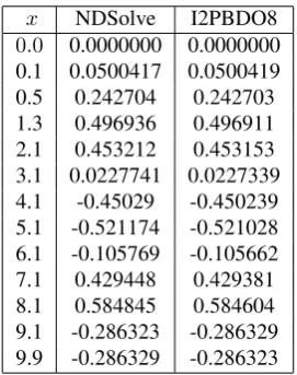
Table 5.Numerical results for solving Van Der Pol.

x NDSolve I2PBDO8

0.0 0.0000000 0.0000000 0.1 0.0500417 0.0500419 0.5 0.242704 0.242703 1.3 0.496936 0.496911 2.1 0.453212 0.453153 3.1 0.0227741 0.0227339 4.1 -0.45029 -0.450239 5.1 -0.521174 -0.521028 6.1 -0.105769 -0.105662 7.1 0.429448 0.429381 8.1 0.584845 0.584604 9.1 -0.286323 -0.286329 9.9 -0.286329 -0.286323

found using I2PBDO8 are compared with the numerical solu-tions obtained in theMathematicabulit in packageNDSolve. Table5 shows the comparison in the numerical approximation ofyat different points ofx.

In addition, Figure 2, depicts the numerical approximations for the the equation in [0,10]. It is obtained by I2PBDO8 with

h = 0.1 which agree very well with the solution obtained

byMathematicabulit in packageNDSolve

Figure 2.Plot of solution for Van Der Pol.

5

Discussion

We presented the numerical results of new method com-pared to the existing methods in tables. The basis for comparison with these methods is chosen because the order of the numerical methods presented in the separate works is either equal or higher to that of the new method. The data given in tables, show the superiority of I2PBDO8 in a term of accuracy.

For the Bessel’s IVP, we have considered the seventh or-der hybrid block method in [17], the variable-step Falkner method of eighth order implemented in a predictor-corrector mode in [18], the eighth order two-step block hybrid third derivative method with one off-step point in [19] and the ninth order four step block hybrid collection method in [20]. In Table 1, comparison in term of absolute errors for different number of steps have been considered at x=8 which made by using our new method with previously literature methods. For problem 2, the numerical results have been obtained by consideringh = 10j_{, j = −2,−4which show maximum}

absolute errors compared to the variable step-size Jator’s block method (VJATOR). Table 2 shows evidence for the good performance of the proposed method.

For problem 3 and 4, we have considered the eight order block methods, implicit linear multistep Hybrid Block method of Uniform order 8 in [21] and uniform order eight implicit block method in [22]. It is observed from Table 3 and 4 that the new method has better accuracy compared with previously existing methods [21] and [22].

In Figure 2 and Table 5, for the Van Der Pol problem, it is obvious that the solutions obtained by I2PBDO8 with step size h = 0.1 agree very well with the observation of

[image:6.595.98.234.482.654.2]

6

Conclusions

In this paper, we have developed the two-point block method with the third and fourth derivatives of the solution for directly solving general second order ODEs. The method has shown a significant improvement in accuracy. Therefore, it can be concluded that the method constructed is suitable for solving general second order ODEs.

Acknowledgements

The authors would like to thank the Universiti Putra Malaysia for the financial support of Putra grant (project No GPB/2017/9543500).

REFERENCES

[1] E. HAIRER AND G. WANNER , A theory for Nystrom methods, Numer. Math., 25 (1976), pp. 383–400.

[2] Chawla, M. M. and Sharma, S. R. (1985). ”Family of Three-Stage Third Order RungeKutta-Nystrom methods for yM=f(x,y,y’)”, Journal of the Australian mathematical society, 26, 375- 386.

[3] Gear, C. W. (1971a). ”Algorithm 407: DIFSUB for solution of ODEs”, Communications of the ACM, 14, 185- 190.

[4] Vigo-Aguiar, J.,& Ramos, H. (2006). Variable stepsize imple-mentation of multistep methods for y = f (x, y, y’). Journal of Computational and Applied Mathematics, 192(1), 114-131.

[5] Awoyemi, D. O. (1999). A class of continuous methods for gen-eral second order initial value problems in ordinary differential equations. International Journal of Computer Mathematics, 72(1), 29-37.

[6] Akinfenwa, O. A.,and Jator, S. N., and Yao, N. M. (2013). Continuous block backward differentiation formula for solving stiff ordinary differential equations. Computers & Mathematics with Applications, 65(7), 996-1005.

[7] Kayode, S. J., & Awoyemi, D. O. (2005). A 5-step maximal order method for direct solution of second order ordinary differential equations. Journal of the Nigerian Association of Mathematical Physics, 9(1), 279-284.

[8] Jator, S. N. (2007). A SIXTH ORDER LINEAR MULTISTEP METHOD FOR. International Journal of Pure and Applied Mathematics, 40(4), 457-472.

[9] Jator, S. N., & Li, J. (2009). A self-starting linear multistep method for a direct solution of the general second-order initial value problem. International Journal of Computer Mathematics, 86(5), 827-836.

[10] Awoyemi, D. O., Adebile, E. A., Adesanya, A. O., & Anake, T. A. (2011). Modified block method for the direct solution of second order ordinary differential equations. International Journal of Applied Mathematics and Computation, 3(3), 181-188.

[11] Cash, J. R. (1981). High orderP-stable formulae for the numer-ical integration of periodic initial value problems. Numerische Mathematik, 37(3), 355-370.

[12] Ismail, G. A., & Ibrahim, I. H. (1999). New efficient second derivative multistep methods for stiff systems. Applied mathe-matical modelling, 23(4), 279-288.

[13] HOJJATI, G.; ARDABILI, MY Rahimi; HOSSEINI, S. M. New second derivative multistep methods for stiff systems. Applied Mathematical Modelling, 2006, 30.5:466-476.

[14] Khalsaraei, M. M., Oskuyi, N. N., & Hojjati, G. (2012). A class of second derivative multistep methods for stiff systems. Acta Universitatis Apulensis, 30, 171-188.

[15] Turki, M. Y., Ismail, F., Senu, N., & Ibrahim, Z. B. (2016, June). Second derivative multistep method for solving first-order ordinary differential equations. In AIP Conference Proceedings (Vol. 1739, No. 1, p. 020054). AIP Publishing.

[16] Henrici, P. (1962). Discrete variable methods in ordinary differential equations.John Wiley and Sons, New York.

[17] Jator, S. N. (2010). Solving second order initial value problems by a hybrid multistep method without predictors. Applied Mathematics and Computation, 217(8), 4036-4046.

[18] Vigo-Aguiar, J.,& Ramos, H. (2006). Variable stepsize imple-mentation of multistep methods for y = f (x, y, y’). Journal of Computational and Applied Mathematics, 192(1), 114-131.

[19] Jator, S. N. (2012). A continuous two-step method of order 8 with a block extension for y = f (x, y, y’). Applied Mathematics and Computation, 219(3), 781-791.

[20] Akinfenwa, O. A. (2013). Ninth order block piecewise con-tinuous hybrid integrators for solving second order ordinary differential equations. International Journal of Differential Equations and Applications, 12(1).

[22] Badmus, A. M. (2014b). A new eighth order implicit block algorithms for the direct solution of second order ordinary differential equations. American Journal of Computational Mathematics, 4(04), 376.

[23] Singh, G., & Ramos, H. (2019). An Optimized Two-Step Hybrid Block Method Formulated in Variable Step-Size Mode for Integrating y= f (x, y, y’) Numerically. NUMERICAL

MATHEMATICS-THEORY METHODS AND APPLICA-TIONS, 12(2), 640-660.