https://doi.org/10.5194/hess-21-4021-2017 © Author(s) 2017. This work is distributed under the Creative Commons Attribution 3.0 License.
Residual uncertainty estimation using instance-based learning with
applications to hydrologic forecasting
Omar Wani1,2,a,b, Joost V. L. Beckers2, Albrecht H. Weerts2,3, and Dimitri P. Solomatine1,4,5
1IHE Delft Institute for Water Education, Delft, the Netherlands 2Deltares, Delft, the Netherlands
3Hydrology and Quantitative Water Management Group, Department of Environmental Sciences, Wageningen University,
Wageningen, the Netherlands
4Water Resources Section, Delft University of Technology, Delft, the Netherlands 5Water Problems Institute of RAS, Moscow, Russia
acurrently at: Institute of Environmental Engineering, Swiss Federal Institute of Technology (ETH), Zürich, Switzerland bcurrently at: Swiss Federal Institute of Aquatic Science and Technology (Eawag), Dübendorf, Switzerland
Correspondence to:Omar Wani ([email protected]) Received: 10 February 2017 – Discussion started: 16 March 2017
Revised: 28 June 2017 – Accepted: 5 July 2017 – Published: 10 August 2017
Abstract. A non-parametric method is applied to quan-tify residual uncertainty in hydrologic streamflow forecast-ing. This method acts as a post-processor on deterministic model forecasts and generates a residual uncertainty distri-bution. Based on instance-based learning, it uses ak nearest-neighbour search for similar historical hydrometeorological conditions to determine uncertainty intervals from a set of historical errors, i.e. discrepancies between past forecast and observation. The performance of this method is assessed us-ing test cases of hydrologic forecastus-ing in two UK rivers: the Severn and Brue. Forecasts in retrospect were made and their uncertainties were estimated using kNN resampling and two alternative uncertainty estimators: quantile regression (QR) and uncertainty estimation based on local errors and clus-tering (UNEEC). Results show that kNN uncertainty estima-tion produces accurate and narrow uncertainty intervals with good probability coverage. Analysis also shows that the per-formance of this technique depends on the choice of search space. Nevertheless, the accuracy and reliability of uncer-tainty intervals generated using kNN resampling are at least comparable to those produced by QR and UNEEC. It is con-cluded that kNN uncertainty estimation is an interesting al-ternative to other post-processors, like QR and UNEEC, for estimating forecast uncertainty. Apart from its concept being simple and well understood, an advantage of this method is that it is relatively easy to implement.
1 Introduction
at getting a range of model outputs, e.g. Beven and Bin-ley (1992) and Freer et al. (1996). Other uncertainty esti-mation techniques may employ a combination of these ap-proaches (Del Giudice et al., 2013). Some techniques focus on one source of uncertainty, such as the model parameter uncertainty (Benke et al., 2008) or the model structure un-certainty (Butts et al., 2004), while others focus on com-bined uncertainties stemming from model parameters, model structure deficits and inputs (Schoups and Vrugt, 2010; Evin et al., 2013; Del Giudice et al., 2013). In this context, it is important to note that apart from estimating uncertainty of model parameters during calibration, uncertainty estimation for hydrologic forecasting requires quantification of predic-tive uncertainty, which includes uncertain system response in addition to different combinations of model parameters (Renard et al., 2010; Coccia and Todini, 2011; Dotto et al., 2012).
In this paper, we will restrict ourselves to the class of un-certainty estimators called post-processors. These methods usually do not discriminate between different sources of un-certainty. They “aggregate” all sources into a so-called resid-ual uncertainty. Post-processing methods assume the exis-tence of a single calibrated model with an optimal set of model parameters, and build a statistical or machine learn-ing model of the residual uncertainty. Typically, these tech-niques relate a combination of model inputs and/or outputs to the model error distribution. Various post-processors have been developed and applied to hydrologic modelling, such as a meta-Gaussian error model (Montanari and Brath, 2004), UNEEC (Solomatine and Shrestha, 2009), quantile regres-sion (Weerts et al., 2011), and DUMBRAE (Pianosi and Raso, 2012). Quantile regression (QR) is a relatively straight-forward post-processing technique that relates the probabil-ity of residual errors to the model forecast (the predictand) by a regression model that is derived from historical fore-casts and observations. QR has been successfully applied for uncertainty quantification in hydrologic forecasts with vari-ous modifications (Weerts et al., 2011; Verkade et al., 2013; Roscoe et al., 2012; López López et al., 2014; Hoss and Fis-chbeck, 2015), whereas UNEEC involves a machine learn-ing technique for buildlearn-ing a non-linear regression model of error quantiles (Solomatine and Shrestha, 2009). UNEEC in-cludes three steps: (1) fuzzy clustering of input data in the space of “relevant” variables; (2) estimating the probabil-ity distribution function of residual errors for each cluster and (3) building a machine learning model (e.g. an artificial neural network) of the prediction interval for a given prob-ability (Dogulu et al., 2015). Many other uncertainty esti-mation techniques, such as DUMBRAE (Pianosi and Raso, 2012), HUP (Krzysztofowicz, 1999), model conditional pro-cessor (Coccia and Todini, 2011), Bayesian revision (Reg-giani et al., 2009) and Bayesian model averaging (Raftery et al., 2005), make explicit assumptions about the nature of the probability distribution function of error. This is not neces-sary for QR and UNEEC (López López et al., 2014; Dogulu
et al., 2015). Nevertheless, in QR and UNEEC assumptions need to be made about the form of the regression function that is used to calculate the quantiles.
In an attempt to explore the utility of easier-to-implement post-processing techniques, we employ a simple non-parametric forecast method for residual uncertainty quan-tification. This method uses kNN search to learn about the past residual errors, which avoids having to make explicit assumptions about the nature of the error distribution and tuning of distribution parameters. Instance-based learning has been used in meteorology and hydrology before for re-sampling of precipitation and streamflows, most notably by Lall and Sharma (1996), who used theknearest-neighbour (kNN) method for resampling of monthly streamflow se-quences. kNN search has also been used in a non-parametric simulation method to generate random sequences of daily weather variables (Rajagopalan and Lall, 1999). They de-fined a weighting function for probability where the pre-dictand is resampled from k values. Jules and Buishand (2003) used nearest-neighbour resampling to generate multi-site sequences of daily precipitation and temperature in the Rhine basin. Also, instance-based learning has been used as a data-driven model for hydrologic forecasting (Soloma-tine et al., 2008; Soloma(Soloma-tine and Ostfeld, 2008). Beckers et al. (2016) use nearest-neighbour resampling to generate monthly sequences of climate indices and related precipita-tion and temperature series for the Columbia River basin. Specifically in the context of error modelling, a version of UNEEC that uses kNN instance-based learning as its ba-sic machine learning technique to predict the residual error quantiles was compared to the original ANN-based UNEEC in Shrestha and Solomatine (2008). However, kNN can also be used without the complicated UNEEC procedure that in-cludes fuzzy clustering. The application of kNN has recently been tested for forecast updating by constructing a determin-istic error prediction model (Akbari and Afshar, 2014). Sim-ilarly, it has been shown that model errors can be resampled using kNN, after explicitly accounting for input and param-eter uncertainty, to generate uncertainty intervals (Sikorska et al., 2015). In this paper we extend the simplification of kNN resampling for uncertainty estimation. We present an application of the kNN method to generate residual uncer-tainty estimates for a predictand, using a fixed time series of input and fixed model parameters, and explore whether this approach, being simpler than many other uncertainty quan-tification approaches mentioned above, is a useful or even a better alternative.
analysed in the first case study. The second case study is used to further validate the performance of kNN uncertainty es-timation and analyse its sensitivity to the choice of search space and the value of k. Also, the influence of systematic bias in the hydrologic model on the uncertainty intervals gen-erated by kNN search is explored in the second case study. For both case studies, performance indices of kNN resam-pling are compared to those of QR and UNEEC. And finally in Sect. 4, we discuss the usability of kNN search as a post-processor uncertainty estimator in hydrologic forecasting.
2 Method
2.1 kNN error model
The kNN residual uncertainty estimator can be seen as a zero-order local error quantile model built from a kNN search. Let us define a vector v inn-dimensional space of variables (the search space) on which the residual uncertainty is assumed to be statistically dependent.
v=
h
v1, . . ., vn
i
(1) The cumulative probability distribution function C of residual errors at prediction time steptconditioned onv=vt is defined as
Ct(e|v=vt)=Pt(E≤e|v=vt) , (2) whereP is the probability function andEdenotes the ran-dom variable for residual errors. Residual error is defined throughout this paper as the difference between the simu-lated values and the observed values for a hydrologic system responsef, like discharge or water level.
e=fsimluated−fobserved (3)
We are making the assumption of stationarity in time so that past error distributions are representative of the future: Ct(e|v=vt)=Cp(e|v=vt) . (4) The subscript p denotes historical time series. ThereforeCp
is the cumulative distribution function of residual errors from the past. In Eq. (4),Cpis being conditioned to the input
vari-able vector at time t. Nevertheless, as we only have single realizations of the error variableEfor each historical point, we relax the constraint ofv=vt. Instead, we assume that the nearby neighbours ofvt inn-dimensional space will have a similar probability distribution of errors tovt and that these historical errors are samples fromCp(e|v=vt). An empiri-cal probability distribution can thus be constructed using the kNN historical errors:
Ct(et|v=vt)≈Cp e|rp≤ rk
[image:3.612.317.537.65.222.2]
, (5)
Figure 1.Dependence of error samples on the value ofk. For larger values ofk, points are at a greater distance from vt (the predic-tion step), thus compromising the condipredic-tioning of the residual error probability distribution onvt(Eq. 5).
whererpis the Euclidean distance inn-dimensional space of
input variables.
rp= |vp−vt| =
v u u t
" n
X
i=1
vi
p−vti
2
#
(6)
vpis the input variable vector of the past data point in the
cloud of such past data pointsv(Fig. 1) andrkis the distance to thekth nearest neighbour of vt. The choice of the input variable vector is a problem in itself since it should include only the most relevant variables that determine the forecast uncertainty. In this study, the input variable vector is cho-sen based on correlation between the candidate variables and the past errors. If the correlation between the error time se-ries and a particular candidate variable is relatively high, then it can be included in the input variable vector space. Other, more sophisticated methods involving the mutual informa-tion can be used as well (Fernando et al., 2009). This will be exemplified in the case studies described in the next section. To represent the relative importance of input variables used in the search, dimensions of the input variable vector space can be suitably weighted in. Also, the model-based methods can be used where models are built for each considered candidate input variable set, and the choice is made based on their rela-tive performance. These, however, were not explored in this study; it rather focused on the usability of the kNN search in its most basic implementation for uncertainty quantifica-tion. Nevertheless, we do demonstrate the sensitivity of the uncertainty intervals to the choice of input variable vector.
in-put variableicalculated using the past data, then
rp= v u u u u t n X i=1
vip−vti
2
σi2
. (7)
Once the input variable vector space is decided, the proba-bility of non-exceedance of a forecast error is calculated em-pirically by sampling from the conditional error distribution: Ct(et|v=vt)≈Cp e|rp≤ rk=j/ k, (8) wherej is the rank of value e (for which the probability of non-exceedance is being computed) in the ascending array ofkerror values. The kNN search is thus employed to gen-erate a sample and to build an empirical error distribution for this predictive uncertainty quantification. Such a mathemat-ical description does not employ explicit regression models for predicting quantiles, which can be seen as a disadvantage in extrapolating outside available data. Also, as this configu-ration of kNN used in this research generates residual error quantiles, which capture the mismatch between measurement values and simulated values, the uncertainty in observational data is not considered. The generated quantiles are aimed at capturing the measured system response and do not attempt to capture the true response of the hydrologic system.
As one would expect, due to the nature of our sampling approximation (Eq. 8), the number of nearest neighbours,k, will affect the empirical conditional probability distribution of errors. Ifkis very large, many data points that are quite distant from vt (Fig. 1) will be selected and the condition-ing on the current forecast situation will not be valid. Large values ofkwill thus yield error distributions with larger un-certainty intervals – resembling the marginal error distribu-tion. Ifkis small, the set ofkerrors will be small and subject to sampling error, so this set will not adequately represent the uncertainty distribution atvt. The tail of a distribution is more prone to sampling errors compared to its mean. Thus, to attain an acceptable degree of convergence, many more samples are required for quantiles corresponding to bigger prediction intervals (van der Vaart, 1998). For improved per-formance, the value of k can be subject to optimization of some cost function: the optimal value ofkcould be the one that enables a reasonable estimate of the uncertainty quan-tiles and additionally we may require that the sensitivity of the error distribution tokis small. In this study, we carry out such optimization using quite a simple heuristic guideline – the value of kis varied until the probability distribution of errors stabilizes and becomes less sensitive to the value ofk for a few model predictions. We also demonstrate the sen-sitivity of uncertainty intervals to the value of k in one of the case studies. The choice of this relatively simple proce-dure for error quantile generation using kNN resampling is a reasonable starting point to assess its potential for residual uncertainty. This study explores the potential of uncertainty
estimation using kNN in as simple a way as possible, and then compares its performance to two other residual uncer-tainty estimators. More advanced application of kNN, for ex-ample using fuzzy weights and kNN sampling to assign pre-diction intervals (Shrestha and Solomatine, 2008) or through explicit consideration of uncertainty in parameter and input by sampling them from their distributions, has been success-fully shown (Sikorska et al., 2015).
To summarize, the steps for uncertainty quantification us-ing kNN resamplus-ing are as follows.
1. Compose the input variable vector space(v)on which uncertainty will be conditioned. Correlation analysis can help find the most relevant variables.
2. Set the number of neighboursk.
3. For a forecast at prediction time stept, identify the set ofknearest neighbours to the input vectorvt. This set represents the hindcasts (forecasts in retrospect) most similar tovt.
4. Use the residual errors from these k points to build an empirical error distribution for the forecast at time stept.
5. Finally, identify the errors corresponding to the required quantiles (probabilities of non-exceedance) from this empirical distribution (in this paper, we use the 5–95 and 25–75 % quantiles).
2.2 Validation methods
Three statistical measures have been employed in this study to check the effectiveness of uncertainty estimation techniques, namely prediction interval coverage probabil-ity (PICPPI), the mean prediction interval (MPIPI) (see e.g.
Shrestha and Solomatine, 2008; Dogulu et al., 2015) and the Alpha Index (Renard et al., 2010). PICPPIrepresents the
per-centage of observations (C) covered by a prediction interval (PI) corresponding to a certain probability of occurrence (in our case 90 and 50 %).
PICPPI= Nin Nobs
·100 %, (9)
whereNinis the number of observations located within the PI
andNobsis the total number of observations. These metrics
are calculated using the following equations:
PICP90=
1
n
n
X
i=1
C90·100 %,PICP50=
1
n n X
i=1
C50·100 %, (10)
C90=
1, if qi,0.05≤qi≤qi,0.95
0, else
,
C50=
1, if qi,0.25≤qi≤qi,0.75
0, else
whereqi,0.95 andqi,0.05 are values with 95 and 5 %
proba-bilities of non-exceedance at timei. Thus the region bound within these two values will have a confidence interval of 90 %. Similarly,qi,0.75 andqi,0.25 represent the boundaries
for 50 % C. The MPI is the average width of the confi-dence intervals corresponding to a particular probability. It is a measure of the magnitude of the uncertainty.
MPI90=
1 n
n
X
i=1
qi,0.95−qi,0.05
MPI50=
1 n
n
X
i=1
qi,0.75−qi,0.25 (12)
We also quantify the reliability of the predicted error quan-tiles by comparing it to the observed error quanquan-tiles. The mis-match between the observed (qobs, j) and predicted (j/100) error quantiles can be summarized by the Alpha Index (α).
α0= 1
100
100 X
j=1
qobs, j−j/100
(13)
α=1−2α0 (14)
There have been discussions whether an isolated verifica-tion index can capture all the aspects that make a probabilis-tic forecast good or bad (Laio and Tamea, 2007). The choice of a verification index for an uncertainty estimation tech-nique should also be dependent on the purpose of hydrologic forecast. For example, Coccia and Todini (2011) evaluate the performance of model conditional processors for flood fore-casting using the predicted and observed probabilities of ex-ceedance over a threshold. Also, in their study predicted error quantiles are compared to observed error quantiles. López López et al. (2014) and Dogulu et al. (2015) use PICP and MPI, among other verification measures, to access the per-formance of QR and UNEEC. This study will limit the com-parison of kNN resampling with other techniques to PICP and MPI only, which give a reasonable assessment of perfor-mance. Nevertheless, it does not preclude the possibility that the uncertainty estimation techniques perform differently if evaluated using other indices.
3 Case studies
The performance of kNN resampling was evaluated by ap-plying the technique to hydrological forecasting for several catchments in two different parts of England. The two case studies provide two different hydrologic conditions for test-ing and include different models for prediction. Also, differ-ent kinds of system responses are being predicted in the two case studies – water level and discharge. The accuracy of the quantified prediction intervals was deduced by using valida-tion data sets. Also, the first case study was used to evaluate the impact of changing lead time on uncertainty of hydro-logic models and its quantification using kNN resampling.
0 20 40 km
Catchment Urban area
[image:5.612.312.546.66.209.2]Forecasting locationRiver stream
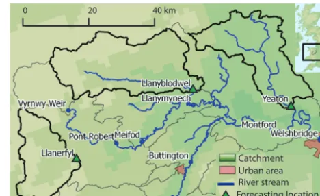
Figure 2.Upper Severn subcatchments with gauging stations (from López López et al., 2014).
3.1 Upper Severn catchment 3.1.1 Catchment description
The Upper Severn region is located in the Midlands, UK (Fig. 2). The River Severn, with a total length of 354 km, is the longest river in the UK. Its course acts as a geographic delineation between England and Wales, finally draining into the Bristol Channel. The overall River Severn catchment area is 10 459 km2. Around 2.3 million people live in this region. The area is predominantly rural, but there are also a num-ber of highly urbanized parts. The area covering the upper reaches of the River Severn, from its source on Plynlimon to its confluence with the River Perry upstream of Shrewsbury in Shropshire, is called the Upper Severn catchment. The Up-per Severn catchment is predominantly hilly. It is dominated on the western edge by the Cambrian Mountains and a sec-tion of Snowdonia Nasec-tional Park (River Severn CFMP; EA, 2009).
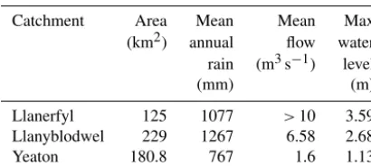
Table 1.Basin information for Upper Severn subcatchments (EA, 2013; Marsh and Hannaford, 2008).
Catchment Area Mean Mean Max
(km2) annual flow water rain (m3s−1) level
(mm) (m)
Llanerfyl 125 1077 >10 3.59
Llanyblodwel 229 1267 6.58 2.68
Yeaton 180.8 767 1.6 1.13
3.1.2 Experimental set-up
The flood forecasting system for the River Severn is orga-nized in a sequential manner, being composed of a number of separate systems that are effectively linked. This forecasting system works with a high degree of automation and efforts have been made to involve a minimum amount of human in-tervention. The UK Environment Agency uses the Midlands Flood Forecasting System (MFFS) to do flood forecasting and to help in warning operation. The MFFS in turn is based on the Delft-FEWS (Flood Early Warning System) platform (Werner et al., 2013). Within the MFFS, there are lumped nu-merical models for rainfall–runoff (MCRM; Bailey and Dob-son, 1981) and models for hydrologic (DODO; Wallingford, 1994) and hydrodynamic routing (ISIS; Wallingford, 1997). The rainfall input for the MFFS is acquired from ground measurements via rain gauges, from radar measurements or from numerical weather prediction data. The MFFS predicts ahead in time the response of the Upper Severn subcatch-ments but, as expected, the quality of forecast deteriorates with increasing lead time.
To do uncertainty analysis for the MFFS, hindcasting or reforecasting is done and then results are compared to the observed data. All the input time series used for hindcasting are taken from measured data. In this study, the reforecasting period was kept equal to the one employed in the studies of López López et al. (2014) and Dogulu et al. (2015). The cho-sen period is from 1 January 2006 to 7 March 2013. Data in the period till 6 March 2007 are used for the model spin-up. The remaining period is used for the calibration and valida-tion of the uncertainty estimavalida-tion techniques. Forecasts are made on a 12-hourly basis – at 08:00 and 20:00 daily, up to a lead time of 48 h. kNN resampling was applied for fore-casts at 10 different lead times: 1, 3, 6, 9, 12, 18, 30, 36, 42, and 48 h. To choose an input variable vector for kNN resam-pling, correlation analysis was done between residual error and contenders for input variable vector space, namely sim-ulated water level (Hsim), measured water level (Hobs) and residual error (Eobs) from various time stepst. The analysis was done to assist in a manual selection of input variable vectors. The correlation between residual error and water level reduces fast with time lag between the two time series.
Therefore it is enough to choose relatively simple and small-dimensional input variable vector spaces. For lead times,l, up to 6 h we chose
v=hHtsim, Ht−lobs, etobs−li. (15)
For higher lead times, uncertainty has only been conditioned onHtsimas the residual error becomes less and less correlated with variable values as measured several hours behind the prediction time.
v=
h
Htsim
i
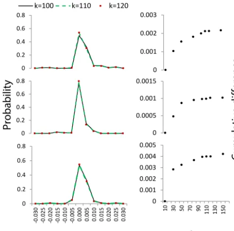
(16) Ninety-nine values of residual errors were sampled from the nearest neighbourhood to generate an empirical distri-bution at each prediction step. This allowed us to get the “resolution” of 1 percentile in the generated empirical dis-tribution. To develop confidence in the chosen value ofk, we checked for a few prediction steps how sensitive the gener-ated empirical distribution is to the value ofk. Four different instances ofvt were chosen. Each instance represents a pre-diction step in the input variable vector space (the red circle in Fig. 1), with different hydrologic conditions. The plots of the cumulative mean square difference between probability density functions (pdfs) of varyingkwere generated. Cumu-lative mean square difference (Eq. 17) serves as an index to show how much the empirical pdfs change with changingk. We get a decreasing slope with increasingk. It shows that the pdfs become almost identical for values ofkaround 100. If Pki(e)is the probability density for a residual errore
calcu-lated throughki nearest neighbours using kNN resampling, for probability functions corresponding to discrete bin size 1e, the cumulative difference is defined as
cumulative difference
=
ki=k X
ki=10
lastebin X
firstebin
1e·Pki(e)−1e·Pki−1(e)
2
. (17)
The various values ofki that were tested are−10, 30, 50, 70, 90, 100, 110, 130 and 150. Using the information from Fig. 3, a value ofk=99 does not seem to be heavily affected by sampling errors. Nevertheless, it is not a mathematically calibrated value ofkand therefore is likely to be sub-optimal. However, it should still be able to provide reasonably repre-sentative samples from the error distribution, as is suggested by Fig. 3.
3.1.3 Results
0 0.001 0.002 0.003 0 0.2 0.4 0.6
0.8 k=100 k=110 k=120
0 0.2 0.4 0.6 0.8 -0 .0 30 -0 .0 25 -0 .0 20 -0 .0 15 -0 .0 10 -0 .0 05 0. 00 0 0. 00 5 0. 01 0 0. 01 5 0. 02 0 0. 02 5 0. 03 0 0 0.001 0.002 0.003 0.004 0.005
10 30 50 70 90 110 130 150
0 0.0005 0.001 0.0015 0 0.2 0.4 0.6 0.8
Cu
m
ul
at
iv
e
d i
ffe
re
nc
e
Pr
oba
bil
ity
[image:7.612.49.287.66.301.2]Error
k
Figure 3.Dependence of the residual error probability function on the value ofkfor three didactic values ofvt (in each row in this plot). The probability is computed for error bins of size 0.005 units each. The graphs show that forkfrom around 90 to 120, the corre-sponding empirical error distributions become almost identical.
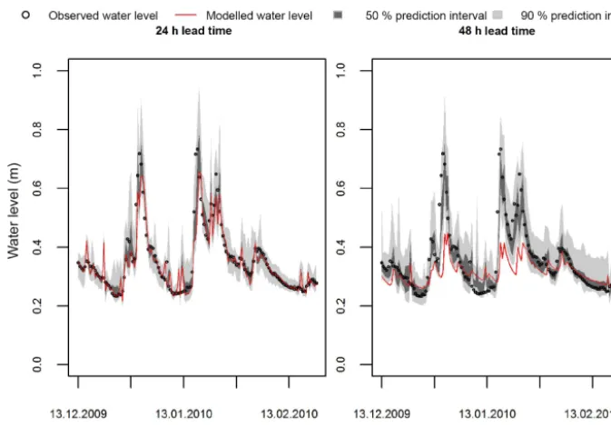
outside the predicted quantiles. This is because kNN resam-pling learns from past instances where the model has consis-tently underpredicted or overpredicted the flow, so it corrects for this bias. The hydrographs capture the low flows and the peaks well. It can also be seen that for high flows the errors are usually higher than for medium and low flows. The resid-ual error distribution is thus heteroscedastic, i.e. the variance depends on the magnitude of the predicted flow. The auto-correlation can be checked by plotting errors versus time, whereas performance of an error model with regard to het-eroscedasticity can be estimated by plotting reliability dia-grams for different magnitudes of flow, which would mean different water levels in this case.
The plotting of error time series (Fig. 5) for various lead times shows some recurring trends across all three subcatch-ments. The errors are small for small lead time forecasts and the spread of error time series increases with increasing lead time. Moreover, the errors do not look autocorrelated for smaller lead times, whereas for the higher lead times auto-correlation becomes more prominent. This can be ascribed to the memory of the hydrologic system. If the system re-sponse is higher than what the model simulates for a particu-lar lead time, then the system response is likely to be higher for the next time step as well. As the errors become larger, they tend to lose their independence property. This is cap-tured by the error samples generated by kNN resampling as well. The rate at which autocorrelation deteriorates for
ob-Table 2.Alpha Index (α) for high flows corresponding to different lead times of Upper Severn subcatchments.
Lead time (h) 1 12 24 48
Llanerfyl 0.92 0.87 0.79 0.64 Llanyblodwel 0.93 0.95 0.93 0.90
Yeaton 0.97 0.94 0.94 0.75
served residual errors corresponds well to the kNN resam-pling error samples’ autocorrelation. It can be seen that kNN resampling preserves the autocorrelation in the error time se-ries without using an autoregressive model.
To check the performance of kNN resampling for various flow magnitudes, the simulation values were divided into low and high flows – the lowest and highest 10 % of water levels simulated in the validation phase respectively. The reliability diagrams (Fig. 6) show that the overall performance of error quantiles for all water levels is good for low and medium lead times. The reliability decreases with high lead times (24 h and above). The reliability plots show that kNN resampling performs better for high flows compared to low flows, even for higher lead times. For low flows and high lead times, the forecast probability of non-exceedance is higher than the ob-served relative frequency. Nevertheless, from 0.90 probabil-ity of non-exceedance and above, the reliabilprobabil-ity curve comes back to the desired 45◦line. For flood forecasting it is impor-tant to model the high and medium flows well. kNN resam-pling delivers quite reliable quantiles for such flow regimes. The deteriorating model performance with higher lead times gets reflected in the performance of kNN resampling quin-tiles as well.
[image:7.612.339.514.96.152.2]Figure 4.Prediction intervals for the Yeaton catchment using kNN resampling. The hydrographs are shown for the two different lead times. The 50 % prediction interval is the interval between the 25 and 75 % quantiles of residual error, and the 90 % quantile is the interval between the 5 and 95 % quantiles. The reporting time interval is 12 h.
made for three locations and five lead times for the valida-tion. For each location and each lead time, the 90 and 50 % quantiles were generated, which allowed for the evaluation of PICP and MPI 30 times (Fig. 7). The PICP of kNN resam-pling is higher in 60 % of the cases and the MPI is smaller in 36 % of the cases. Based on these results we concluded that, for this case study, kNN resampling generally produces narrower confidence bands and provides a better coverage of the probability distribution than the other methods in the ma-jority of forecasts, especially showing better performance for the larger lead times.
3.2 River Brue
3.2.1 Catchment description
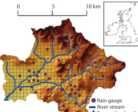
The River Brue, located in the south-west of England, has a history of severe flooding. The test forecast location used in this study is Lovington, where the upstream catchment area is 135 km2(Fig. 8). The catchment is predominantly rural and the soil consists of clay and sand. This kind of soil and the modest relief give rise to a slowly responsive flow regime. The mean annual rainfall in the catchment is 867 mm; the mean river flow is 1.92 m3s−1and has a maximum flow of 39.58 m3s−1. This catchment has been extensively used for
research on weather radar, quantitative precipitation forecast-ing and hydrologic modellforecast-ing.
3.2.2 Experimental set-up
Figure 6. Reliability diagram from Upper Severn subcatchments for(a)low,(b)high and(c)all flows (Llanerfyl: blue; Llanyblod-wel: green; Yeaton: red).
Figure 7.PICP and MPI comparison for Upper Severn subcatch-ments –(a)Llanerfyl,(b)Llanyblodwel and (c) Yeaton.
three input variable vectors used are
v(ivv1)=hQsimt i, (18)
v(ivv2)=
h
Qsimt , eobst−1i, (19)
v(ivv3)=
h
Rtobs−8, Rt−obs9, Robst−10, Qobst−1, Qobst−2, Qobst−3,
eobst−1, etobs−2 i
, (20)
[image:10.612.47.287.75.661.2]sim-Rain gauge
Forecasting location River stream
[image:11.612.52.286.66.256.2]0 5 10 km
Figure 8.Brue catchment (from Shrestha and Solomatine, 2008).
ulated and observed values respectively. The number of near-est neighbours was chosen to be 99 and 199, to analyse its influence on uncertainty quantification. Uncertainty analysis was done for a calibrated HBV model as well as a model with a unit systematic bias. The bias was introduced to the simu-lation results of the calibrated model by simple addition. The aim of a biased model for uncertainty quantification using kNN resampling is to assess the performance of kNN resam-pling when the residuals are not zero mean.
3.2.3 Results
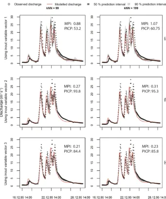
kNN resampling was applied to a single historical simulation and compared to observations. The simulated hydrographs for the highest discharge event with 50 and 90 % predic-tion intervals are shown in Fig. 9. The residual distribupredic-tion of kNN resampling is generally a non-zero mean. Therefore we see that the prediction intervals may sometimes deviate from the deterministic model prediction quite significantly. The ability of kNN resampling to search for similar hydro-logic conditions, like rainfall, and discharge in the past, and to learn from the residuals, allows it to make more represen-tative error distributions. For example, in Fig. 9, the falling limb of the hydrograph shows that the prediction band gen-erated by kNN resampling captures the observed flow for in-put variable vectors 2 and 3, even though the model shows a noticeable mismatch with the measurements. This can be explained by considering the history of errors that the model made during such hydrologic conditions in the past. And as kNN resampling learns that the model consistently underes-timates in such cases, the corresponding error distribution corrects for this bias. The results of the PICP and MPI are shown in Table 3 together with results from UNEEC and QR (Dogulu et al., 2015). As can be seen from the table, kNN re-sampling’s performance is comparable to that of UNEEC and
QR for this case study. The prediction intervals generated by kNN resampling are smaller, compared to the other two un-certainty estimation techniques, while the coverage probabil-ity is similar. It indicates that kNN resampling is able to learn well from past data and condition the probability of residual errors well. The Alpha Index for the validation phase is also high (0.96). We also notice that three different input variable vectors show different degrees of performance (Fig. 9). The past errors,etobs−1, seem to be informative in this case, provid-ing very narrow conditional error probabilities.
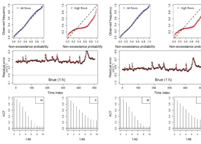
Apart from evaluating the usability of kNN resampling for calibrated models, the performance of kNN resampling quan-tiles generated by kNN resampling for a model with system-atic bias was also checked. Figure 10 shows that the perfor-mance of kNN resampling does not diminish under system-atic bias. The reliability of the generated quantiles remains almost unfazed. As a systematic bias will not affect the au-tocorrelation structure of the residual errors, the autocorre-lation of error samples generated through kNN resampling also remains unchanged. Nevertheless, we see a shift in the mean of the sample time series, which is roughly equal to unity. The reliability of quantiles generated using kNN re-sampling for high flows (highest 10 % in the validation pe-riod) is poorer than for all flows. The invariance of kNN re-sampling performance to model bias makes it a robust post-processor technique; however, unlike in the case of Upper Severn subcatchments, the technique’s performance dimin-ishes for high flows.
4 Discussion and conclusions
distribu-Figure 9.The 50 and 90 % prediction intervals for the Brue catchment using kNN resampling. The hydrographs are shown for two different
[image:12.612.133.474.63.470.2]kvalues (99, 199) and three different input variable vectors given by(a)Eq. (18),(b)Eq. (19) and(c)Eq. (20). This is the largest event in the validation time series. (The 50 % prediction interval is the interval between the 25 and 75 % quantiles of residual error, and the 90 % quantile is the interval between the 5 and 95 % quantiles. MPI and PICP correspond to the whole validation time series.)
Table 3.Performance of various uncertainty estimation techniques for the Brue catchment. For kNN resampling and UNEEC the same input variable vector is used (Eq. 20). For QR onlyQsimis used.
PICP MPI
(expected 90 %) (m3s−1)
UNEEC QR kNN UNEEC QR kNN
Calibration 91.19 90.00 86.3 1.58 1.69 0.51
Validation 88.29 82.33 84.42 1.37 1.39 0.21
tion mean, thus maintaining the performance of prediction intervals. Our results on systematic error correction by kNN resampling substantiate the findings from previous research on forecast updating using kNN (Akbari and Afshar, 2014).
[image:12.612.167.427.572.645.2]Figure 10.Effect on reliability of quantiles and autocorrelation of error samples on adding a systematic bias to the model artificially. kNN samples, generated using input variable vector 3 (Eq. 20), are plotted in red, and observed errors in black circles. M stands for measured and S for simulated.
(MPIs) generated by kNN resampling are generally smaller. A significantly smaller MPI using kNN resampling, as in the case of the Brue, is in part due to the conditioning on in-put variable vectors as compared to UNEEC and QR. As the values ofk in this study have been restricted to 99 and 199, the error distribution tends to be much narrower than the marginal error distribution. The conditional distribution will turn into a marginal distribution when the number ofkis equal to the time steps in the calibration time series. A more quantitative dependence on the k value and MPI will need further research. Apart from a narrow MPI, we also find that kNN resampling is generally able to capture the expected ra-tio of observara-tions within its intervals (PICP) most of the time, or at least be close to the expected value.
As in the case of all other data-driven methods, the ap-plicability of kNN resampling depends on the availability of sufficiently long and representative historical forecasts and observations. The historical series should include several oc-currences of forecasting situations that are similar to the cur-rent situation. In extreme cases, the kind of kNN search pro-posed here will select the most similar historical situations which may or may not be representative of the current situ-ation. In contrast to the methods like QR and UNEEC that build explicit predictive regression models which are able to extrapolate for the data which are beyond the limits of the
calibration (training set), kNN resampling does not extrap-olate. This could be seen as a disadvantage. On the other hand, however, the extrapolation that is done by regression techniques could also be seen as doubtful. It is not a given that the most extreme historical situations are less represen-tative of the uncertainty of an extremely high flow than an extrapolated result. The results in this paper show that kNN resampling has a good or poor reliability for the highest val-ues in the validation set, depending on the case study and the choice of input variable vector. Due to the non-parametric nature of kNN resampling, the increasing variance of resid-ual errors for higher values of predictands is generally ade-quately taken into account.
One of the few calibration parameters of kNN resampling is the number of nearest neighboursk. In this study,k has been chosen by a simple heuristic technique. For optimal performance, it would be advisable to calibrate k for each application in a more systematic way. We do show for Brue that the sensitivity of the uncertainty intervals to the value of kis not significant, when changing it from 99 to 199. How-ever, we also expect that the optimal value ofkwill depend on the length of the historical data series and on the uncer-tainty quantiles of interest. In the context of search space, in this research, the input variable vector has been chosen by correlation analysis. It can be recommended to use more so-phisticated procedures for real-life applications, which can capture the non-linear dependence between the error process and input variable vector candidates. Improvements in per-formance can possibly be achieved by seeking a better set of input variables for each forecast location and lead time of interest.
In conclusion, kNN resampling can be considered a rela-tively simple machine learning technique to predict hydro-logic residual uncertainty. The errors from the similar hy-drologic conditions in the past are used as samples for the residual error probability distribution and the samples are collected by a k nearest-neighbour search. The application of this technique to case studies Brue and Upper Severn sub-catchments has shown promising results. In comparison to many other data-driven techniques, kNN resampling has the advantage of avoiding assumptions about the nature of the residual error distribution: the instance-based learning ap-proach is non-parametric and non-regressive and requires lit-tle calibration. The method was shown to be able to quan-tify hydrologic uncertainty to an accuracy that is compa-rable to other techniques like QR and UNEEC. Given the relatively small effort in setting up the method, the perfor-mance of kNN resampling in uncertainty quantification is more than acceptable when compared to other post-processor error models.
5 User interface
A website has been developed as part of this research to help generate uncertainty intervals using kNN resam-pling for a given time series of predictions. Address: www. modeluncertainty.com.
Data availability. Data are available upon request.
Competing interests. The authors declare that they have no conflict of interest.
Acknowledgements. The authors would like to acknowledge Bonneville Power Administration, Portland, USA, for supporting this research. The UK Environment Agency is acknowledged for provision of the data for the case studies described in this paper. Many thanks to Nilay Dogulu, Patricia López López, Marijn Swenne, and Azam Iftikhar for their help during the course of this research. We are thankful to Sven Eggimann and Heuning Badger in helping structure the paper. Finally, we are grateful to the editor, Bettina Schaefli, and two reviewers for their valuable comments. Part of this study was supported by EC FP7 project WeSenseIt (Citizen Observatory of Water), grant agreement no. 308429, by the Russian Science Foundation (grant no. 17-77-30006), and project QUICS (Quantifying Uncertainty in Integrated Catchment Studies), grant agreement no. 607000.
Edited by: Bettina Schaefli
Reviewed by: José Matos and Luciano Raso
References
Akbari, M. and Afshar, A.: Similarity-based error prediction ap-proach for real-time inflow forecasting, Hydrol. Res., 45, 589– 602, https://doi.org/10.2166/nh.2013.098, 2014.
Arnal, L., Ramos, M.-H., Coughlan de Perez, E., Cloke, H. L., Stephens, E., Wetterhall, F., van Andel, S. J., and Pappenberger, F.: Willingness-to-pay for a probabilistic flood forecast: a risk-based decision-making game, Hydrol. Earth Syst. Sci., 20, 3109– 3128, https://doi.org/10.5194/hess-20-3109-2016, 2016. Bailey, R. A. and Dobson, C.: Forecasting for floods in the
Sev-ern catchment, Journal of the Institution of Water Engineers and Scientists, 35, 168–178, 1981.
Beckers, J. V. L., Weerts, A. H., Tijdeman, E., and Welles, E.: ENSO-conditioned weather resampling method for seasonal en-semble streamflow prediction, Hydrol. Earth Syst. Sci., 20, 3277–3287, https://doi.org/10.5194/hess-20-3277-2016, 2016. Benke, K. K., Lowell, K. E., and Hamilton, A. J.: Parameter
un-certainty, sensitivity analysis and prediction error in a water-balance hydrological model, Math. Comput. Model., 47, 1134– 1149, https://doi.org/10.1016/j.mcm.2007.05.017, 2008. Bergström, S.: Development and application of a conceptual runoff
model for Scandinavian catchments, Swedish Meteorological and Hydrological Institute, Norrköping, Sweden, SMHI Rep. RHO 7, 134 pp., 1976.
Beven, K. and Binley, A.: The future of distributed models: Model calibration and uncertainty prediction, Hydrol. Process., 6, 279– 298, https://doi.org/10.1002/hyp.3360060305, 1992.
Butts, M. B., Payne, J. T., Kristensen, M., and Madsen, H.: An eval-uation of the impact of model structure on hydrological mod-elling uncertainty for streamflow simulation, J. Hydrol., 298, 242–266, https://doi.org/10.1016/j.jhydrol.2004.03.042, 2004. Coccia, G. and Todini, E.: Recent developments in predictive
uncertainty assessment based on the model conditional pro-cessor approach, Hydrol. Earth Syst. Sci., 15, 3253–3274, https://doi.org/10.5194/hess-15-3253-2011, 2011.
uncertain-ties in urban drainage models, Phys. Chem. Earth Pt. A/B/C, 42– 44, 3–10, https://doi.org/10.1016/j.pce.2011.04.007, 2012. Del Giudice, D., Honti, M., Scheidegger, A., Albert, C., Reichert, P.,
and Rieckermann, J.: Improving uncertainty estimation in urban hydrological modeling by statistically describing bias, Hydrol. Earth Syst. Sci., 17, 4209–4225, https://doi.org/10.5194/hess-17-4209-2013, 2013.
Dogulu, N., López López, P., Solomatine, D. P., Weerts, A. H., and Shrestha, D. L.: Estimation of predictive hydrologic uncer-tainty using the quantile regression and UNEEC methods and their comparison on contrasting catchments, Hydrol. Earth Syst. Sci., 19, 3181–3201, https://doi.org/10.5194/hess-19-3181-2015, 2015.
Dotto, C. B. S., Mannina, G., Kleidorfer, M., Vezzaro, L., Henrichs, M., McCarthy, D. T., Freni, G., Rauch, W., and Deletic, A.: Com-parison of different uncertainty techniques in urban stormwa-ter quantity and quality modelling, Wastormwa-ter Res., 46, 2545–2558, https://doi.org/10.1016/j.watres.2012.02.009, 2012.
EA: Environment Agency: River levels: Midlands, available at: http://www.environment-agency.gov.uk/homeandleisure/floods/ riverlevels/ (last access: 1 October 2013), 2009.
Evin, G., Kavetski, D., Thyer, M., and Kuczera, G.: Pitfalls and im-provements in the joint inference of heteroscedasticity and au-tocorrelation in hydrological model calibration, Water Resour. Res., 49, 4518–4524, https://doi.org/10.1002/wrcr.20284, 2013. Fernando, T. M. K. G., Maier, H. R., and Dandy, G.
C.: Selection of input variables for data driven mod-els: An average shifted histogram partial mutual infor-mation estimator approach, J. Hydrol., 367, 165–176, https://doi.org/10.1016/j.jhydrol.2008.10.019, 2009.
Freer, J., Beven, K., and Ambroise, B.: Bayesian Estimation of Un-certainty in Runoff Prediction and the Value of Data: An Applica-tion of the GLUE Approach, Water Resour. Res., 32, 2161–2173, https://doi.org/10.1029/95WR03723, 1996.
Gupta, H. V., Sorooshian, S., and Yapo, P. O.: Toward improved calibration of hydrologic models: Multiple and noncommensu-rable measures of information, Water Resour. Res., 34, 751–763, https://doi.org/10.1029/97wr03495, 1998.
Hoss, F. and Fischbeck, P. S.: Performance and robustness of prob-abilistic river forecasts computed with quantile regression based on multiple independent variables, Hydrol. Earth Syst. Sci., 19, 3969–3990, https://doi.org/10.5194/hess-19-3969-2015, 2015. Jules, J. B. and Buishand, T. A.: Multi-site simulation of daily
pre-cipitation and temperature conditional on the atmospheric circu-lation, Clim. Res., 25, 121–133, 2003.
Krzysztofowicz, R.: Bayesian theory of probabilistic forecasting via deterministic hydrologic model, Water Resour. Res., 35, 2739– 2750, https://doi.org/10.1029/1999WR900099, 1999.
Krzysztofowicz, R.: The case for probabilistic forecasting in hy-drology, J. Hydrol., 249, 2–9, https://doi.org/10.1016/S0022-1694(01)00420-6, 2001.
Laio, F. and Tamea, S.: Verification tools for probabilistic fore-casts of continuous hydrological variables, Hydrol. Earth Syst. Sci., 11, 1267–1277, https://doi.org/10.5194/hess-11-1267-2007, 2007.
Lall, U. and Sharma, A.: A Nearest Neighbor Bootstrap For Resam-pling Hydrologic Time Series, Water Resour. Res., 32, 679–693, https://doi.org/10.1029/95wr02966, 1996.
Li, H., Luo, L., Wood, E. F., and Schaake, J.: The role of initial conditions and forcing uncertainties in seasonal hydrologic forecasting, J. Geophys. Res., 114, D04114, https://doi.org/10.1029/2008jd010969, 2009.
Lindström, G., Johansson, B., Persson, M., Gardelin, M., and Bergström, S.: Development and test of the distributed HBV-96 hydrological model, J. Hydrol., 201, 272–288, https://doi.org/10.1016/S0022-1694(97)00041-3, 1997. López López, P., Verkade, J. S., Weerts, A. H., and Solomatine, D.
P.: Alternative configurations of quantile regression for estimat-ing predictive uncertainty in water level forecasts for the upper Severn River: a comparison, Hydrol. Earth Syst. Sci., 18, 3411– 3428, https://doi.org/10.5194/hess-18-3411-2014, 2014. Marsh, T. and Hannaford, J.: UK hydrometric register, Hydrological
data UK series, Centre for Ecology and Hydrology, Wallingford, UK, 1–210, 2008.
Montanari, A. and Brath, A.: A stochastic approach for assess-ing the uncertainty of rainfall-runoff simulations, Water Resour. Res., 40, W01106, https://doi.org/10.1029/2003WR002540, 2004.
Pianosi, F. and Raso, L.: Dynamic modeling of predictive uncer-tainty by regression on absolute errors, Water Resour. Res., 48, W03516, https://doi.org/10.1029/2011WR010603, 2012. Raftery, A. E., Gneiting, T., Balabdaoui, F., and Polakowski,
M.: Using Bayesian Model Averaging to Calibrate Fore-cast Ensembles, Mon. Weather Rev., 133, 1155–1174, https://doi.org/10.1175/mwr2906.1, 2005.
Rajagopalan, B. and Lall, U.: A k-nearest-neighbor simulator for daily precipitation and other weather variables, Water Resour. Res., 35, 3089–3101, https://doi.org/10.1029/1999wr900028, 1999.
Refsgaard, J. C., van der Sluijs, J. P., Hojberg, A. L., and Vanrol-leghem, P. A.: Uncertainty in the environmental modelling pro-cess – A framework and guidance, Environ. Modell. Softw., 22, 1543–1556, https://doi.org/10.1016/j.envsoft.2007.02.004, 2007. Reggiani, P., Renner, M., Weerts, A. H., and van Gelder, P. A. H. J. M.: Uncertainty assessment via Bayesian revision of ensemble streamflow predictions in the operational river Rhine forecasting system, Water Resour. Res., 45, W02428, https://doi.org/10.1029/2007WR006758, 2009.
Reichert, P., Borsuk, M., Hostmann, M., Schweizer, S., Spörri, C., Tockner, K., and Truffer, B.: Concepts of decision support for river rehabilitation, Environ. Modell. Softw., 22, 188–201, https://doi.org/10.1016/j.envsoft.2005.07.017, 2007.
Renard, B., Kavetski, D., Kuczera, G., Thyer, M., and Franks, S. W.: Understanding predictive uncertainty in hydrologic modeling: The challenge of identifying input and structural errors, Water Resour. Res., 46, W05521, https://doi.org/10.1029/2009WR008328, 2010.
Roscoe, K. L., Weerts, A. H., and Schroevers, M.: Esti-mation of the uncertainty in water level forecasts at un-gauged river locations using quantile regression, Interna-tional Journal of River Basin Management, 10, 383–394, https://doi.org/10.1080/15715124.2012.740483, 2012.
Shrestha, D. L. and Solomatine, D. P.: Data-driven approaches for estimating uncertainty in rainfall-runoff modelling, Inter-national Journal of River Basin Management, 6, 109–122, https://doi.org/10.1080/15715124.2008.9635341, 2008. Sikorska, A. E., Alberto, M., and Demetris, K.: Estimating
the Uncertainty of Hydrological Predictions through Data-Driven Resampling Techniques, J. Hydrol. Eng., 20, A4014009, https://doi.org/10.1061/(ASCE)HE.1943-5584.0000926, 2015. Solomatine, D. P. and Ostfeld, A.: Data-driven modelling: some
past experiences and new approaches, J. Hydroinform., 10, 3– 22, https://doi.org/10.2166/hydro.2008.015, 2008.
Solomatine, D. P. and Shrestha, D. L.: A novel method to estimate model uncertainty using machine learn-ing techniques, Water Resour. Res., 45, W00B11, https://doi.org/10.1029/2008WR006839, 2009.
Solomatine, D. P., Maskey, M., and Shrestha, D. L.: Instance-based learning compared to other data-driven methods in hydrological forecasting, Hydrol. Process., 22, 275–287, https://doi.org/10.1002/hyp.6592, 2008.
Todini, E.: A model conditional processor to assess pre-dictive uncertainty in flood forecasting, International Journal of River Basin Management, 6, 123–137, https://doi.org/10.1080/15715124.2008.9635342, 2008. van Andel, S. J., Weerts, A., Schaake, J., and Bogner,
K.: Post-processing hydrological ensemble predictions in-tercomparison experiment, Hydrol. Process., 27, 158–161, https://doi.org/10.1002/hyp.9595, 2013.
van der Vaart, A. W.: Asymptotic Statistics, Asymptotic Statistics, 3, 443 pp., https://doi.org/10.2307/2530729, 1998.
Verkade, J. S., Brown, J. D., Reggiani, P., and Weerts, A. H.: Post-processing ECMWF precipitation and temper-ature ensemble reforecasts for operational hydrologic fore-casting at various spatial scales, J. Hydrol., 501, 73–91, https://doi.org/10.1016/j.jhydrol.2013.07.039, 2013.
Wallingford: Wallingford Water, a flood forecasting and warning system for the river Soar, Wallingford Water, Wallingford, UK, 1994.
Wallingford: HR Wallingford, ISIS software, HR Wallingford, Hy-draluic Unit, Wallingford, UK, available at: http://www.isisuser. com/isis/ (last access: 1 October 2013), 1997.
Weerts, A. H., Winsemius, H. C., and Verkade, J. S.: Estima-tion of predictive hydrological uncertainty using quantile re-gression: examples from the National Flood Forecasting Sys-tem (England and Wales), Hydrol. Earth Syst. Sci., 15, 255–265, https://doi.org/10.5194/hess-15-255-2011, 2011.