Global spatial optimization with hydrological systems simulation: application to land use allocation and peak runoff minimization

www.hydrol-earth-syst-sci.net/14/325/2010/ © Author(s) 2010. This work is distributed under the Creative Commons Attribution 3.0 License.

Hydrology and

Earth System

Sciences

Global spatial optimization with hydrological systems simulation:

application to land-use allocation and peak runoff minimization

I.-Y. Yeo1and J.-M. Guldmann2

1_{Department of Geography, The University of Maryland, College Park, Maryland, USA} 2_{Department of City and Regional Planning, The Ohio State University, Columbus, Ohio, USA} Received: 30 March 2009 – Published in Hydrol. Earth Syst. Sci. Discuss.: 28 April 2009 Revised: 5 January 2010 – Accepted: 8 January 2010 – Published: 18 February 2010

Abstract. A general methodology is presented to integrate complex simulation models of hydrological systems into op-timization models, as an alternative to scenario-based ap-proaches. A gradient-based hill climbing algorithm is pro-posed to reach locally optimal solutions from distinct start-ing points. The gradient of the objective function is esti-mated numerically with the simulation model. A statistical procedure based on the Weibull distribution is used to build a confidence interval for the global optimum. The method-ology is illustrated by an application to a small watershed in Ohio, where the decision variables are related to land-use al-locations and the objective is to minimize peak runoff. The results suggest that this specific runoff function is convex in terms of the land-use variables, and that the global optimum has been reached. Modeling extensions and areas for further research are discussed.

1 Introduction

Understanding watershed hydrological processes and their linkages to land cover changes is important for controlling nonpoint source (NPS) water pollutants, which are produced by land-based activities (Novotny, 2003) and carried into wa-terways by stormwater runoffs. Effective management of NPS pollution calls for methods to identify pollution sources and pathways, and to minimize pollutants production and delivery. Computer simulation models of complex water-shed processes can provide a better understanding of the in-teractions among the various physical systems in a water-shed, and predict the hydrological impacts of changes in land

Correspondence to: I.-Y. Yeo ([email protected])

management practices (Beven, 1989; Grayson et al., 1992). They have been used to develop Best Management Practices (BMP) and to predict the effects of future climate changes (Quilb´e et al., 2008).

However, these simulation models necessarily consider only a small number of scenarios, precluding the optimal se-lection and location of BMPs, and cannot explicitly link pol-lution sources to yields. Optimization methods have recently emerged as an alternative modeling framework to efficiently search for the best possible alternative, under given objec-tives (performance measures) and constraints (Haith, 1995). Srivastava et al. (2002), Nicklow and Muleta (2001), Muleta and Nicklow (2002), Seppelt and Voinov (2002), and Kaur et al. (2004) have integrated optimization methods into simula-tion models to overcome the limitasimula-tions of a scenario-based approach. However, there is little evaluation of the obtained solution in terms of its closeness to the global one (Lee and El-Sharkawi, 2008). This would require a thorough under-standing of the relationship between the watershed system and the decision variables.

The purpose of this research is primarily to propose a gen-eral methodology for the efficient use of simulation models of natural systems within an optimization framework. These simulation models can be viewed as implicit functions re-lating inputs to outputs, with some inputs representing deci-sion variables and the outputs representing favorable and/or unfavorable impacts. The methodology is illustrated with a hydrological runoff simulation model applied to a small catchment in Ohio, and the decision variables are related to land-use allocation. The optimization procedure involves the simulation-based numerical approximation of gradient vec-tors at each step of a hill-climbing algorithm. A large num-ber of local optima is generated, and the Weibull distribution is used to statistically assess convergence towards the global optimum.

326 I.-Y. Yeo and J.-M. Guldmann: Global spatial optimization The remainder of this paper is organized as

fol-lows. Section 2 describes the methodology, including the optimization-simulation procedure and the statistical as-sessment of local optima using the Weibull distribution. Section 3 describes an application of the methodology, in-cluding the data, the hydrological simulation model, the re-sults for a small catchment, and model extensions. The structure of the peak runoff function is further analyzed in Sect. 4 in light of the underlying mechanics of the hydrolog-ical model. Conclusions and areas for further research are presented in Sect. 5.

2 Methodology

2.1 Optimization-simulation procedure

Most natural systems (hydrological, atmospheric, or ecolog-ical) can be represented by simulation models of varying de-grees of sophistication and complexity. The inputs to these models include exogenous variables, decision variables, and parameters. In the specific case of NPS pollutants/runoff models, these could be:

E= vector of exogenous variables, such as the geographic distributions of soil types, topography, shallow aquifers, sur-face stream network, channel length, and weather (precipi-tation, temperature, solar radiation, wind speed, relative hu-midity). For a given site/region, these variables cannot be modified, at least in the short and middle terms, and are taken as given;

X= vector of decision variables, which represent various possible management and planning interventions, such as the allocation of land uses, the sitting and sizing of eco-logical engineering technologies (e.g., constructed wetlands or filtration systems), rainwater harvesting, and agricultural practices (application and management of nutrients and pes-ticides, conservation tillage, contour farming, crop residue management, irrigation);

P= vector of the parameters that characterize the various equations/relationships that make up the simulation model (e.g., CN number, Manning’s coefficient, canopy intercep-tion of precipitaintercep-tion, etc.).

LetY be the vector of the simulation outputs. Assume that there arenoutputs, withY=(Y1Y2....Yk...Yn). In the case of watershed simulation models such as the SWAT (Soil and Water Assessment Tool) model (Arnold et al., 1998),Y

includes the (1) peak runoff, (2) sediment load, (3) phos-phorous load, and (4) nitrogen load. These outputs can be watershed-wide aggregates, or disaggregated by location (e.g., Hydrologic Response Unit – HRU). The simulation model can be symbolically represented by the vector func-tionF=(F1,F2...Fk...Fn), with:

Y=F(E,X,P). (1)

The functional relationship (1) is implicit and cannot be expressed in closed mathematical form because of the spatial and temporal complexity of the simulation model, which is generally run for a discrete number of scenarios pertaining to the decision vector X, and/or for different geographical settings (vectorsE andP). Various technological, environ-mental, and socio-economic constraints must be accounted for, that limit the feasible space forX, with:

G(E,X,P )≤O. (2)

A variety of objective functions may be considered. For instance, letYk be the peak runoff at the watershed outlet, and assume that the only goal is to minimize this runoff. Then, the problem is to findXthat minimizes

Yk=Fk(E,X,P) (3)

subject to constraint (2). Some of the other outputs (e.g., pollutant loads) may be constrained by pollution standards

Y∗

j(maximum load or maximum concentration), with:

Fj(E,X,P)≤Y∗j. (4)

Finally, in the context of multi-objective optimization, the search for the Pareto frontier of non-inferior solutions (Co-hon, 1978) involves the minimization of the weighted func-tion (wi≥0):

L=X

i

wiYi=

X

i

wiFi(E,X,P). (5)

For the sake of exposition simplicity, ignore the exogenous components E and P. Let F(X) be the unidimensional function to be minimized. Consider an algorithmic process wherein a sequence of solution pointsXk={x_jk}is generated. Consider the vectorZ={zj}in the neighborhood of thek-th trial pointXk_{. The functionF (Z) can be approximated in} this neighborhood by the following linear function based on a first-order Taylor’s series expansion:

F (Z)≈FXk+ J

X

j=1

∂F (Xk) ∂xj

zj−xjk

. (6)

With Xk _{fixed, F(Z) is linear in Z. However, this linear} approximation is not straightforward to obtain, because the objective function is not analytically closed, and the partial derivatives must be approximated numerically. The∂F (Xk₎ change inF Xk

programming, also known as the method of convex combina-tions (Venkataraman, 2001). If the constraints are nonlinear, various gradient-based feasible directions algorithms can be used (Bazaraa et al., 2006).

In the case of minimization, the algorithm produces the globally optimal solution only if (1) the constraint domain is convex, and (2) the objective function is convex over the feasible domain, which requires that its Hessian matrix be positive definite everywhere (Intriligator, 1976). The Hes-sian matrix is made up of the second-order partial derivatives of the objective function. Since the objective function cannot be expressed analytically, it is impossible to directly assess its convexity. In order to keep the focus on the objective func-tion, assume that the constraint set is convex. The algorithm is presumed to generate a locally optimal solution for each distinct starting point (initial solution). Using a large number of different initial solutions, two situations may emerge:

(1) the same local optimum is obtained in all cases, which indicates that the functionF is convex and the global opti-mum has been found; or

(2) distinct local optima are obtained, which indicates that the function is not convex; in this case, a probabilistic method is proposed in Sect. 2.2 to assess the closeness of the best local optimum to the global optimum.

The complexity and computational requirements of the proposed methodology beg the following question: why is it important to obtain the global optimal solution, and why would a good solution be insufficient? There are two funda-mental reasons for searching for the global optimum. First, using simulation only would necessarily lead to a limited number of solutions, which may all be significantly inferior. In any case, it would be difficult to assess the quality of a so-lution, unless the global optimum is known. Second, maybe more importantly, the global optimum is the benchmark to be used when assessing heuristic procedures that yield good, but not necessarily optimal solutions. Heuristics are much less computationally demanding, but have no value if they cannot be evaluated. The operations research literature has offered many heuristics for difficult-to-solve optimization problems (Pearl, 1984).

A second issue is related to the uncertainty in the inputs

P andE. This uncertainty has been alleged to make the search for an optimum meaningless. For instance, Beven and Freer (2001) discuss the concept of equifinality, whereby the same outputY can be obtained with different sets of the inputsP andE, which are characterized by measurement or other uncertainties. However, uncertainty is a very gen-eral modeling issue, characterizing both natural and socio-economic systems models. It can be tackled, in part, through sensitivity analyses of the solution over ranges of parameter values, or with stochastic programming techniques. The fo-cus of the proposed methodology is not on the vectorsP/E

but on the vector X – the management/planning decision variables.

2.2 Statistical assessment of local optima

It is possible to assess how close a local optimum is to the global one by using a statistical method developed by Golden (1978) and Los and Lardinois (1982). The idea is to generate independent local optima and to obtain a point esti-mate for the global optimum by applying statistical extreme-value theory. Golden (1978) investigates how far a heuristic solution is from the global optimum in the case of the trav-eling salesman problem. Los and Lardinois (1982) apply a hill-climbing technique to solve the optimal network design problem.

The local optima generated from different initial states are analyzed with the Weibull Distribution (WD), which has been used to analyze survival data, to assess stability, and to measure risk (Aitkin and Clayton, 1980). In hydrology, the WD has been used to fit hydrographs (Bhunya et al., 2006) and analyze trends in extreme events, including annual peak discharges, annual minimum flows, and annual maximum rainfall intensities (Clarke, 2002). One of its advantages is its independence from the parent distribution. Parent distri-bution assumptions are often critical in constructing a con-fidence interval (CI), because they help derive the statistical parameters that determine the lower and upper bounds of a CI. However, the optimization algorithm only provides ex-treme values (maximum or minimum), and the underlying probability distribution is unknown. The WD does not re-quire any assumptions to derive the probability of the ex-treme values, as long as there are enough available data (Roberts, 1971). It is derived as the asymptotic distribution of the smallest order statistics, known as Type III (Fisher and Tippett, 1928; Gumbel, 1958). Its cumulative distribution function8(x)and density functionδ(x)are:

8(x)=1−exp

−

_x−a

b

c

(7)

δ (x)=c b

_x−

a b

c−1

exp

−

_x−

a b

c

, (8)

x≥a >0;c >0,b >0.

The parametersa,b, andcare defined as the location, scale, and shape parameters, with8(a+b)=1−e−1(≈0.63). The parametera, the lower bound of the WD, is also the lower bound of the parent-distribution, and is considered the global optimum (minimum). The best local optimum is used as an estimate of the global optimum, and its reliability is statis-tically evaluated by analyzing the empirically fitted WD of local optima. IfRobservations (i.e., sample size) are drawn from a WD, and ifx_(l)h , the best local optimum, is the first element (i.e., smallest number) in an ordered set, it follows that:

P r{x_(l)h ≤a+b} =1−P r{x_(l)h > a+b}

=1−{1−8_xh

(1)(a

+b)}{1−8_xh

(2)(a

+b)}...

{1−8_xh

(R)(a

+b)} =1−(e−1)R=1−e−R.

(9)

328 I.-Y. Yeo and J.-M. Guldmann: Global spatial optimization The estimator_bafor the location parameterais used as point

estimator for the global optimum (_bx∗). Its confidence inter-val, with a significance level of 100(1-e−R)%, is (Golden and Alt, 1979; Dergis, 1985):

P r{x_(l)h −bb≤_bx∗ ≤x_(l)h } ≈1−e

−R_{. (10)}

However, the interval calculated by this formula is too large. It was tightened by Los and Lardinois (1982), using a real numberV, with:

8(a+b/V )=1−exp−(1/V )c. (11)

Then, the confidence interval is given as:

P rnx_(l)h −bb/V≤_bx∗ ≤xh_(l) o

=1−exp −R/Vc. (12)

The confidence level (1-α) is expressed as

1−exp −R/Vc=1−α, (13)

and the real numberV is

V=(−R/ lnα)1/bc. (14)

Estimating the global optimum value and its confidence in-terval can then be used to assess convergence toward the global optimum.

3 Application

3.1 Data

The Old Woman Creek (OWC) watershed, part of the Na-tional Estuarine Research Reserve (NERR) system, is se-lected for a pilot study because of the availability of the de-tailed physical and socio-economic data needed to develop, parameterize, and validate the model. Data on watershed characteristics was collected from remote sensing images, historical land use maps, soil maps from the soil survey geographic database (SSURGO), technical reports from the NERR center, and farmer surveys from the local USDA-NRCS (US Department of Agriculture, Natural Resources Conservation Service) office. These data, which provide a comprehensive description of surface characteristics, are used to derive proper values for the model parameters.

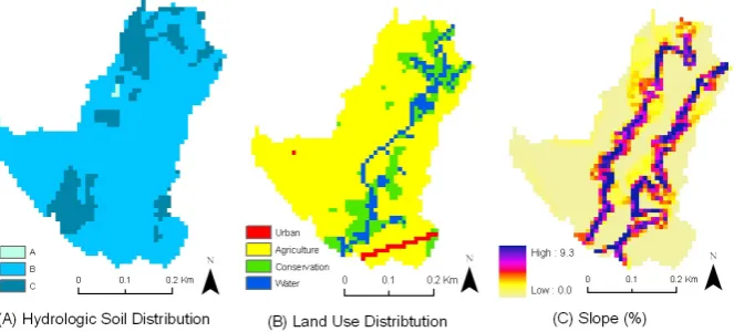
Due to the large computing requirements and the need to generate many independent local optima, the numerical ap-plication is performed on a small catchment of the OWC wa-tershed, with a few land-use categories, a simple drainage network, and simple spatial distributions of land uses and soil types. The catchment is overlaid by a grid of 1732 30-m cells (approximately 1.6 km2), with land-use/cover classified into three categories: agriculture, conservation, and urban. The catchment is predominantly agricultural (78%), conservation land uses (grass/woods) represent 12.6 % of the area, urban land use makes up 1.5%, and the remainder represents wa-ter (8%). Roads make up most of the urban land (25 cells),

except for one cell of built-up structures. The land-use, soil, and topography structures of the catchment are illustrated in Fig. 1. See Yeo et al. (2004) for further descriptions of the OWC and data sources and processing.

3.2 Hydrological simulation model

The relationshipF (X) between a land-use patternXand the resulting peak discharge rate at the watershed outlet is ana-lyzed with a spatially explicit hydrological model, by mod-ifying the SCS curve number (CN) method. This method has been chosen, because (1) the relationship between land-use and peak runoff is expressed in terms of hydrologic soil groups and land use/cover conditions (McCuen, 1982; USDA, 1986; Bingner and Theurer, 2001), (2) it is imple-mentable under available computing resources, and (3) it is simple and accurate. The CN method has been embedded into various watershed models for hydrology, flood analysis, and water quality modeling (Garen and Moore, 2005), in-cluding the Soil and Water Assessment Tool (SWAT) (Arnold et al., 1998), the AGricultural Non-Point Source Pollution Model (AGNPS) (Bingner and Theurer, 2001; Young et al., 1989), and the Erosion Productivity Impact Calculator or the Environmental Policy Integrated Climate (EPIC) model (Williams et al., 1984; Williams and Meinardus, 2004). There have been continuous efforts to modify the CN values under different physiographic and climatic conditions (Ponce and Hawkins, 1996; Arnold and Fohrer, 2005; Grunwald and Frede, 1999), and to merge the CN method with distributed, variable source area concepts (Walter and Shaw, 2005).

The conventional CN method yields lumped effects by us-ing weighted averages of the parameters. To better account for the impacts of spatial variability in land use, a 30-m cell is selected as the modeling unit, consistent with the smallest spatial resolution for a number of input data, including soil, land use, and DEM. Therefore, the spatial heterogeneity and variability of the input data are fully considered, and lump-ing is minimized by not uslump-ing average input values at the cell level. The volume of runoff (Q) is computed as:

Q=(P−0.2S)

2

P+0.8S , (15)

whereP is the precipitation andS the moisture retention, estimated from the runoff curve number (CN):

S=254

₁₀₀

CN−1

. (16)

The quantities P, Q, and S are measured in millimeters [mm]. Groundwater flows are not modeled, and the an-tecedent soil moisture condition is considered by using the default estimation of the SCS method (USDA, 1986). Details are provided in McCuen (1982), USDA (1986), and Bingner and Theurer (2001).

28 Figure 1: Characteristics of the Study Area

Note: The hydrologic soil distribution (soil type A, B ,C, D) is the soil grouping used in the SCS-CN number method, related to the soil infiltration capacity. There is no soil type D in the study site.

Fig. 1. Characteristics of the Study Area. Note: the hydrologic soil distribution (soil type A, B ,C, D) is the soil grouping used in the SCS-CN number method, related to the soil infiltration capacity. There is no soil type D in the study site.

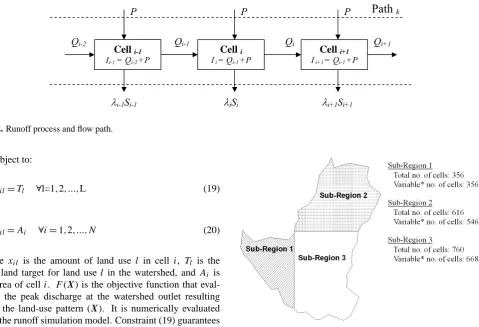
a given cell to the lowest-elevation cell among the eight surrounding cells (O’Callaghan and Mark, 1984). The on-site cell infiltration capacity (i.e., the initial abstraction), which depends only on cell characteristics (soil, land use, antecedent soil moisture), is compared with the precipita-tion depth at the cell, and the excess precipitaprecipita-tion is trans-formed into cell runoff while accounting for the upstream runoff routed through the flow path, in a way similar to the routing method in SWAT (Gassman et al., 2007). The ex-cess runoff over a flow path is then obtained by summing up the storm runoffs occurring at all the cells along the flow path, and the total runoff volume at the watershed outlet is obtained by summing up the runoffs occurring along all flow paths in the watershed (Olivera 1996). This process is illus-trated in Fig. 2.

A similar approach is applied to estimate the time of con-centration, Tc. Instead of computing Tc from a predefined longest distance to the watershed outlet, the model calculates it by keeping track of the flow time of every pathway, to bet-ter account for land spatial variability. The travel time of a flow path is calculated by summing up the travel times for all the cells along the path. The maximum travel time across all paths is selected as the time of concentration. The travel time for each cell is determined according to its flow type – overland flow, shallow concentrated flow, or channel flow (USDA, 1986), which accounts for routing and decay. See the extended TR-55 for details (USDA, 1986; Bingner and Theurer, 2001).

After calculating the time of concentration and the total amount of runoff, the peak runoff rate is determined using the extended TR-55 procedure (Bingner and Theurer 2001), with:

Qp=2.78·10−3P24Da·

"

ap+(cp·Tc)+(ep·Tc2) 1+(bp·Tc)+(dp·Tc2)+(fp·Tc3)

#

(17) whereQp is the peak discharge [m3/s],Da the area of the spatial unit [ha],P24the 24-h effective rainfall over the total

drainage area [mm],Tc the time of concentration [hr], and the coefficientsap,bp,cp,dp,ep, andfp, are determined by the ratio of initial abstraction (Ia) to 24-h precipitation (P24). See Bingner and Theurer (2001) for the values of these coef-ficients.

The hydrological model was calibrated and validated by comparing model output with historic precipitation and stream flow data. First, the daily precipitation data available for the site were fitted using the Extreme Value Type I prob-ability distribution function (Chow et al., 1989) to determine the design storms. Since the data are only available in daily steps, it is assumed that the precipitation pattern follows a SCS II rainfall time distribution (USDA, 1986). Then, the es-timated design storms were used as inputs to the hydrological model, and the peak stream runoffs were simulated and com-pared with the observed stream flows. As the simulation was event-based, a flood frequency analysis was carried out with observed stream data and the Bulletin 17B method (IACWD, 1982). After determined the frequency curve, the stream runoff rates corresponding to the probabilities of 1-, 2-, 5-, and 10-year storms were determined. These stream runoff rates were comparable with the simulation outputs at a 95% confidence level. The flood analysis uses daily stream data over the period 1987–2002. Daily precipitation data were obtained from the National Weather Service Center from the period 1985–2002. See Yeo et al. (2004) for the values used for parameterization and further information on model vali-dation and calibration.

3.3 Land-use optimization model

A simple land use optimization model is integrated with the hydrological model to delineate the land-use pattern that minimizes the peak storm runoff at the watershed outlet:

MinF (X)=Peak Runoff Rate (18)

330 I.-Y. Yeo and J.-M. Guldmann: Global spatial optimization

29 Figure 2: Runoff process and flow path

Qi+1

Qi-1

Celli-1

Ii-1 = Qi-2 +P

Celli

I i = Qi-1 +P

Celli+1

I i+1 = Qi-1 +P

Qi

Qi-2

P P P

λ

λ

λ

Path

Fig. 2. Runoff process and flow path.

Subject to: N

X

i=1

xil=Tl ∀l=1,2,...,L (19)

L

X

l=1

xil=Ai ∀i=1,2,...,N (20)

where xil is the amount of land use l in celli, Tl is the total land target for land use l in the watershed, and Ai is the area of celli. F (X) is the objective function that eval-uates the peak discharge at the watershed outlet resulting from the land-use pattern (X). It is numerically evaluated with the runoff simulation model. Constraint (19) guarantees the achievement of watershed land-use targets, and constraint (20) guarantees the full occupation of celliby land uses. 3.4 Results

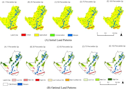
Five hundred land-use maps have been generated by ran-domly assigning land uses to the 1567 catchment cells that are neither road nor water. The total land-use areas are kept constant across these maps: 22 urban cells, 1307 agricultural cells, and 237 conservation cells. These totals correspond to the optimal land allocation in Yeo et al. (2007). The com-bined simulation-optimization model is then applied to these 500 land-use allocations at the 30-m cell level, and the result-ing optimal allocations that minimize peak stormwater runoff at the catchment outlet are further analyzed statistically. Nine identical local solutions obtained from clearly different ini-tial maps were eliminated in order to satisfy the assumptions of the Fisher-Tippett theorem, which requires independence of the observations in the sample (Los and Lardinois, 1982; Dergis, 1985).

In order to illustrate the wide range of the 491 initial so-lutions, the catchment is divided into three sub-regions, as illustrated in Fig. 3, and statistics for the numbers of agri-cultural, conservation, and urban cells allocated to each sub-region are reported in Table 1, confirming that these alloca-tions vary significantly within each sub-region. This range is mirrored by the range of the corresponding peak discharge rates, which vary from 0.25 m3/s to 0.5 m3/s (Fig. 4a). In

Fig. 3. Sub-regions in the OWC Catchment. ∗Denotes cells that are neither water nor road.

Table 1. Summary Statistics for the initial and optimal allocations.

Sub-Region 1 Sub-Region 2 Sub-Region 3

Initial Optimal Initial Optimal Initial Optimal

Statistical Measure Land Use allocation allocation allocation allocation allocation allocation

Mean Urban 5.152 4.192 7.435 9.151 9.413 8.658

Agriculture 298.635 294.271 454.994 470.403 553.371 542.326

Conservation 51.559 54.646 83.571 66.446 101.870 115.908

Median Urban 5.000 4.197 7.000 9.169 9.000 8.639

Agriculture 298.000 294.225 455.000 470.386 553.000 542.314

Conservation 52.000 54.719 84.000 66.391 102.000 115.937

Minimum Urban 0.000 3.217 2.000 7.776 3.000 7.616

Agriculture 282.000 292.932 433.000 467.995 534.000 540.212

Conservation 37.000 53.122 59.000 64.396 77.000 113.875

Maximum Urban 11.000 5.010 14.000 10.655 17.000 10.200

Agriculture 315.000 295.935 481.000 472.956 573.000 544.603

Conservation 68.000 55.852 102.000 69.312 125.000 117.635

Standard Deviation Urban 2.037 0.307 2.359 0.502 2.442 0.432

Agriculture 6.049 0.569 7.151 1.065 7.239 0.711

Conservation 5.580 0.514 6.809 0.874 6.801 0.672

Coefficient of Variation Urban 0.395 0.073 0.317 0.055 0.259 0.050

Agriculture 0.020 0.002 0.016 0.002 0.013 0.001

Conservation 0.108 0.009 0.082 0.013 0.067 0.006

Note: the numbers in the table indicate the number of cells (30-m) assigned to the different land uses.

31

Figure 4: Distributions of the Peak Discharge Rates

0.250 0.3 0.35 0.4 0.45 0.5 20

40 60 80 100 120 140 160

180 Peak Flow Obtained from the Initial Maps

Qp, m3/s

F

req

ue

nc

y o

f

Oc

cu

rr

en

ce

0.254050 0.25410 0.25415 0.25420 0.25425 0.25430 50

100

150 Peak Flow Obtained from the Optimal Maps

Qp, m3/s

F

req

ue

nc

y o

f

Oc

cu

rr

en

ce

(A) Peak flow obtained from the initial maps (B) Peak flow obtained from the optimal maps Qp [m3/s]

Qp [m3/s]

Fre

que

nc

y of Occu

rre

nce

Fre

que

nc

y of Occu

rre

nce

Fig. 4. Distributions of the Peak Discharge Rates.

These optimal peak runoff values are obtained at con-vergence, that is, when the sum of the squared differ-ences between the land allocations of two consecutive iter-ations in the optimization procedure 1XkT

1Xk

is less thanε=10−8. It is very likely that with a much smaller convergence criterionε, the algorithm would converge to the

same optimum for all the initial solutions. However, because the model is gradient-based, the convergence becomes very slow after about 10 iterations, and reaching the exact global optimum might take a huge amount of computing time. In addition, the optimized peak runoffs are extremely close to each other, with differences only at the 6th decimal point.

332 I.-Y. Yeo and J.-M. Guldmann: Global spatial optimization

32

Figure 5

:

Initial and Optimal Land Use Maps

Note: The optimal land maps (4.B) are generated using three land use categories for illustration

purpose only: urban (Urb), Agriculture (Ag), and Conservation (Con). Only the dominant land

use category is coded for each cell, except in the case where two land categories are in the same

density group. Three density groups are used: Low = 0-30 %, Med (medium) = 30-60%, High =

60-100 %.

(A) Initial Land Patterns

(B) Optimal Land Patterns

Fig. 5. Initial and Optimal Land Use Maps. Note: the optimal land maps (4b) are generated using three land use categories for illustration purpose only: urban (Urb), Agriculture (Ag), and Conservation (Con). Only the dominant land use category is coded for each cell, except in the case where two land categories are in the same density group. Three density groups are used: Low=0–30%, Med (medium)=30–60%, High=60–100%.

These differences are meaningless in a physical sense, and make a strong case for global optimality and the convexity of the peak runoff function.

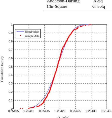
The statistical methodology presented in Sect. 2.2 can be applied to the 491 “optimal” peak discharge rates, which can be viewed as a random sample forε-level convergence. A three-parameter Weibull distribution is estimated and the results are presented in Table 2. The distribution of the sampled data is presented in Fig. 6. The global optimum and its confidence interval (CI) are estimated from the ε -level optimal values, and the results are summarized in Ta-ble 3. The best value from the numerical experiment (i.e.,

x_(l)h or the upper bound of the CI) is 0.254073, approxi-mately 0.01% above the point estimate of the global optimum (_bx∗=0.254047). The lower bound of the CI is 0.254023, about 0.02% below the best local optimum (x_(l)h ).

3.5 Model extensions

Table 2. Data fitting with a weibull distribution.

Parameter Estimation Estimate

Location (Threshold):a 0.254047

Scale:b 0.000156

Shape:c 4.448359

Mean of Sample Data 0.25419

Standard Deviation of Sample Data 0.000034

Minimum of Sample Data 0.254073

Maximum of Sample Data 0.254298

Goodness-of-Fit Tests for Weibull Distribution

Test Statistic P-Value

Cramer-von Mises W-Sq 0.356 Pr>W-Sq 0.084

Anderson-Darling A-Sq 2.593 Pr>A-Sq 0.036

Chi-Square Chi-Sq 42.572 (d.f.=10) Pr>Chi-Sq <0.001

33

Figure 6: Observation vs. Fitted Cumulative Density Function

0.254050 0.25410 0.25415 0.25420 0.25425 0.25430 0.25435 0.1

0.2 0.3 0.4 0.5 0.6 0.7 0.8 0.9 1

fitted value sample data

Qp [m3/s]

Cu

mu

lativ

e Den

sity

Fig. 6. Observation vs. fitted cumulative density function.

Table 3. Estimation for the global optimum and confidence interval.

bx∗ = 0.254047 R= 491

x_(l)h = 0.254073 α= 0.05 (95% CI)

V= 3.1466

x_(n)h = 0.254298 95% CI of_bx∗= (0.254023, 0.254073)

time-independent, land-use pattern subsumed by vectorX, the peak runoff for periodtwould beFt(X), as computed by the simulation model under the conditions of periodt. Min-imizing, for instance, the aggregate annual runoff,P

t Ft(X), could be implemented with the same procedure. It simply would be lengthier and more computationally demanding be-cause gradients would have to be calculated for each period.

The land allocation model is very simplified. It only con-siders total land use targets and land availability per cell, and only one objective – peak runoff minimization. It does not consider other ecological (e.g., carbon fixation, animal and vegetal species preservation, etc.) and socio-economic fac-tors in the watershed. This was done purposefully, to al-low for a focus on the simulation of the peak runoff, and to generate, with the available computer resources, the largest possible set of feasible solutions (land-use allocations) over which to search for the global optimum. Therefore, the obtained minimum peak runoff can be viewed as the lower bound for the minimum peak runoff that would be obtained if more constraints were added to the model. The method-ology could be integrated into a much more comprehen-sive land allocation model, with not only more constraints, but also multiple objectives. There is a literature on multi-objective optimization models applied to watershed issues, but these models are of an aggregate nature and do not deal with detailed allocations at the cell (or HRU) level. For instance, Sadeghi et al. (2009) allocate land to five agri-cultural land uses while minimizing erosion and maximiz-ing economic benefits. Chang et al. (1995) allocate land to forest conservation, agriculture, recreation, and residen-tial development, while minimizing the discharges of five distinct pollutants and maximizing employment and income. Gabriel et al. (2006) develop a mixed-integer quadratic pro-gram to select parcels for development while (1) maximiz-ing the compactness of the development area, (2) minimiz-ing its imperviousness, (3) minimizminimiz-ing the development of environmentally-sensitive parcels, and (4) maximizing the total value of the development parcels.

334 I.-Y. Yeo and J.-M. Guldmann: Global spatial optimization 4 Characterization of the peak runoff function

If the local minimum generated by a hill-climbing algorithm always turns out to be the global one, the objective function is necessarily convex. The previous results suggest that the peak runoff function is convex in terms of the land-use vari-ables. However, as this function cannot be expressed ana-lytically in a closed form, its convexity cannot be proven by analyzing its Hessian matrix. As discussed in Sect. 3, the total runoff volume and travel time are involved in estimat-ing the peak discharge. The effects of the land-use variables on these two components and the whole hydrological system are further examined, to provide additional support (though no formal proof) for the convexity of the objective function. 4.1 Estimation of runoff volume

As described in Eq. (15), the CN method is used to estimate the volume of runoff (Q) as a function of precipitation (P) and moisture retention (S). While precipitation is exogenous to the simulation model,S is solely a function of the curve number (Eq. 16), which is endogenous, as it depends upon land cover and soil type. Letxil be land uselin celli, and cil the curve number for land uselin celli. Since soil types do not vary across the watershed, the curve number (cni) for celliis:

cni=

X

l

cilxil (21)

Therefore, the parameter Si and the runoff volume Qi of celli are functions of the vector of the land-use variables

Xi=(xi1,. . . xil,..xil) , with:

Si=f (Xi) (22)

Qi=g(Xi) (23)

The runoff volumeQpa along the flow pathpato the

water-shed outlet is estimated by summing the runoff volumes in all cellsiin the path, with:

Qpa= X

i∈pa Qi=

X

i∈pa

g(Xi)=

X

i∈pa "

(Pi−0.2f (Xi))2 Pi+0.8f (Xi)

#

=X

i∈pa 

      "

Pi+0.2 P100

l

cilxil−1 !#2

Pi+0.8 P100

l

cilxil −1

! 

     

(24)

Piis the amount of precipitation in celli. The routing path is determined by the D-8 method. Equation (24) is identi-cal to Eqs. (15)–(16), but applies to the runoff volume along the flow path, instead of to a single cell. Although the total runoff is expressed analytically as a function of the land-use variables, it is difficult to characterize the convexity of the

34

Figure 7: Numerical Assessment of Peak Discharge Rate with Varying Curve Number

77 78 79 80 81 82

0.08 0.1 0.12 0.14 0.16 0.17

CN Values

Q

Qp

[m

3/s]

CN value

Fig. 7. Numerical assessment of peak discharge rate with varying curve number.

function presented in Eq. (24), because of the termf (Xi). A numerical analysis has been conducted to better understand this function. With the given land allocation and soil distri-bution (Fig. 1), the CN values (P

l

cilxil) only vary over [77– 82] in the catchment, because most of it is used for agricul-ture and conservation. The runoff volume (Qpa) generated

for these CN values was computed. The results, presented in Fig. 7, show a monotonously increasing and slightly convex relationship betweenQpa and CN. As CN is a linear function

of theXi’s,Qpa is then a convex function of theXi’ s.

4.2 Estimation of runoff travel time

As discussed in Sect. 3.2, the most influential parameters for flow times are land uses and topography. The overland flow is a function of Manning’s roughness coefficient, flow length, and slope; the shallow concentrated flow is determined by slope; the channel flow is computed with Manning’s rough-ness coefficient, channel length and area, and slope. Man-ning’s roughness coefficient, a parameter for surface friction and resistance, is a function of land-cover, and topography determines flow directions, slopes, and drainage patterns.

The hydrological model keeps track of all flow paths to the watershed outlet, and assigns a specific flow type to each cell on each path. This is necessary to account for the im-pacts of site-specific land-use changes, as surface cover af-fects the Manning’s roughness coefficient used in flow time estimation. Then, the flow time is explicitly calculated for each celli, and the total flow time over pathpais estimated as the sum of the travel times over all the consecutive flow segments along the flow path. The time of concentration

I.-Y. Yeo and J.-M. Guldmann: Global spatial optimization 335

35

Figure 8: Regression Coefficients for Peak Discharge (Bingner and Theurer, 2002)

0 0.2 0.4 0.6 0.8 1 0 0.5 1 1.5 2 C oef fi ci en t, a Ia/P24 ratio

0 0.2 0.4 0.6 0.8 1 -2 0 2 4 6 C oe ff ici en t, b Ia/P24 ratio

0 0.2 0.4 0.6 0.8 1 -0.02 0 0.02 0.04 0.06 0.08 C oef fi ci en t, c Ia/P24 ratio

0 0.2 0.4 0.6 0.8 1 -0.1 0 0.1 0.2 0.3 C oef fi ci en t, d Ia/P24 ratio

0 0.2 0.4 0.6 0.8 1 0 0.002 0.004 0.006 0.008 0.01 C oef fi ci ent , e Ia/P24 ratio

0 0.2 0.4 0.6 0.8 1 -5

0 5 10x 10

-3 C oef fi ci ent , f Ia/P24 ratio

Ia/P24ratio

Ia/P24ratio

Ia/P24ratio

Ia/P24ratio

Ia/P24ratio

Ia/P24ratio

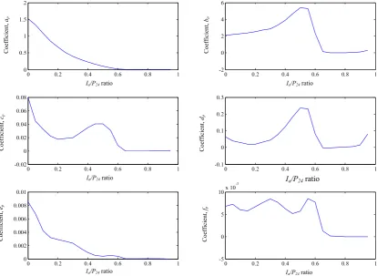
Coefficient, ap Coefficien t, bp Coefficient, cp Coefficient, dp Coefficient, ep Coefficient, fp

Fig. 8. Regression Coefficients for Peak Discharge (Bingner and Theurer, 2002).

variables vectorX:

Tc=H (X) (25)

4.3 Estimation of peak discharge

The peak discharge rate at the watershed outlet is estimated using the extended TR-55 method (Bingner and Theurer, 2002), which requires the following inputs: the runoff vol-ume, the time of concentration, and the unit peak regression coefficientsap−fp. These coefficients are determined by the rainfall distribution and the ratioIa/P24. The initial ab-straction (Ia,i) of celliis estimated as 20% of the moisture retentionSi (Eq. 16), which is itself dependent upon the land uses in celli(USDA, 1986), with:

Ia,i=0.2·Si=0.2

  254    100 P l cilxil

−1     

=y(Xi) (26)

The initial abstraction for the watershed is then estimated as the average value ofIa,i:

Ia/P24=

X

i

Ia,i/P24=

X

i

y(Xi)/P24=Y (X). (27)

The constantsap−fpare derived from a look-up table, and Fig. 8 presents their values as functions of the ratioIa/P24, for Type II rainfall. Except for coefficientap, these curves are strongly nonlinear. Once the values of the parameters

ap−fpare determined, the peak discharge rate is computed as:

Qp=2.78×10−3P24Da·

"

ap+(cp·Tc)+(ep·Tc2) 1+(bp·Tc)+(dp·Tc2)+(fp·Tc3)

#

=2.5×10−2 NP a X

1

QP aL(H (X),Y (X)) (28)

whereY (X) represents the ratioIa/P24 that determines the regression coefficientsap−fp(Eq. 27),H (X) represents the time of concentration Tc (Eq. 25), andNp_ais the number of all possible paths. The right-hand side of Eq. (28) is essen-tially identical to Eq. (17), as the total runoff at the watershed outlet (

NP a P

1

QP a) is equal to the product of the total drainage area by the effective rainfall (P24Da), which is the amount of precipitation that is neither retained by the land surface nor infiltrated into the soils. Equation (28) relates two compo-nents, the total runoff volume and the time of concentration,

336 I.-Y. Yeo and J.-M. Guldmann: Global spatial optimization

36

Figure 9: Numerical Assessment of ( ( ), ( ))L H X Y X Under Type II Rainfall Distribution

0 0.5 1 1.5 2 0.2 0.4 0.6 0.8 1 1.2 1.4 1.6 hr L( H (X) ), Y( X) ) Ia/P24=0.00

0 0.5 1 1.5 2 0.05 0.1 0.15 0.2 0.25 0.3 0.35 0.4 0.45 0.5 hr L( H (X) ), Y( X) ) Ia/P24=0.25

0 0.5 1 1.5 2 0.01 0.02 0.03 0.04 0.05 0.06 0.07 0.08 0.09 0.1 hr L( H (X) ), Y( X) ) Ia/P24=0.50

0 0.5 1 1.5 2 1.54 1.55 1.56 1.57 1.58 1.59 1.6 1.61x 10

-3 hr L( H (X) ), Y( X) ) Ia/P24=0.75

Ia/P24=0.00 Ia/P24=0.25 Ia/P24=0.50 Ia/P24=0.75

L(H( X ), Y ( X )) L (H ( X ), Y ( X )) L (H ( X ), Y ( X )) L (H ( X ), Y ( X ))

Time [hr] Time [hr] Time [hr] Time [hr]

Fig. 9. Numerical Assessment ofL(H (X),Y (X))Under Type II Rainfall Distribution.

to the peak runoff. As the runoff volume ( NP a

P

1

QPa) has been

shown to be convex (Sect. 4.1), Eq. (28) is further analyzed by focusing on the componentL(H (X),Y (X)).

The functionL(H (X),Y (X)) is computed with selected values for Tc and theIa/P24ratio for the study area. Numer-ical results are presented in Fig. 9 forIa/P24=(0.00, 0.25, 0.50, 0.75) and Tc in the range [0–2 h], which covers all pos-sible Tc values in the 500 initial land-use patterns. The re-lationships presented in Fig. 8 are either convex or linear. However, the convexity of Eq. (28) cannot be guaranteed, as the multiplication of two convex functions,L(H (X),Y (X))

and NP a

P

1

QPa, cannot be mathematically proven to be convex.

5 Conclusions

This paper has presented a general methodology for integrat-ing complex simulation models of natural systems into op-timization models that account for various socio-economic and environmental objectives and constraints. In the specific case of hydrological watershed models, the decision vari-ables are related to land-use allocations, sitting and sizing of structural BMPs, agricultural practices, and non-structural BMPs, and the environmental outputs include peak runoff and sediment, phosphorous, and nitrogen loads. The gradi-ent of the objective function is estimated numerically with the simulation model, and a hill climbing algorithm is im-plemented to reach either a local optimum or the global op-timum. A statistical procedure based on the Weibull distri-bution is next used to estimate the global optimum out of a large number of model-generated local optima.

The methodology has been applied with a peak runoff sim-ulation model to the OWC watershed in Ohio. The decision variables are land-use allocations, and the objective is to min-imize peak runoff at the watershed outlet. A large number of solutions has been generated from distinct initial solutions, and these solutions turned out to be very close, strongly sup-porting the case for a convex relationship between peak

dis-charge and land-use variables. The convexity of the objective function has been further investigated by examining the un-derlying mechanics of the hydrological model (i.e., the SCS-CN method) in terms of land-use variables, and by perform-ing numerical evaluations of its main components. The nu-merical results also support, though do not fully prove, the case for convexity.

The methodology can be adapted to deal with other op-timization and simulation models, and to design watershed structural BMPs, alternative agricultural practices, and non-structural BMPs (e.g., use of pervious material in urban areas). The modeling scope can be extended to (1) include multiple storms, and (2) account for socio-economic and other environmental factors. To further assess the method-ology, numerical experimentations should be undertaken with other simulation models, objectives, constraints, and sites/regions. The search for and derivation of the global optimum should provide the basis for designing heuristic procedures that yield very good, though not necessarily optimal, managerial and planning decisions.

Edited by: N. Verhoest

References

Aitkin, M. and Clayton, D.: The fitting of exponential, Weibull and extreme value distributions to complex censored survival data us-ing GLIM, J. Roy. Stat. Soc. C-App., 29(2), 156-163, 1980. Arnold, J. G. and Fohrer, N.: SWAT2000: current capabilities and

research opportunities in applied watershed modeling, Hydrol. Process., 19, 563–572, 2005.

Arnold, J. G., Srinivasan, R., Muttiah, R. S., and Williams, J. R.: Large Area Hydrologic Modeling and Assessment – Part I: Model Development, J. Am. Water Resour. As., 34(1), 73–89, 1998.

Bazaraa, M. S., Sherali, H. D., and Shetty, C. M.: Nonlinear Pro-gramming: Theory and Algorithms, John Wiley & Sons, New York, USA,2006.

Beven, K. J. and Freer, J.: Equifinality, data assimilation, and un-certainty estimation in mechanistic modeling of complex envi-ronmental systems using the GLUE methodology, J. Hydrol., 249(1–4), 11–29, 2001.

Bhunya, P. K., Berndtsson, R., Ojha, C. S. P., and Mishra, S. K.: Suitability of Gamma, Chi-square, Weibull, and Beta distribu-tions as synthetic unit hydrographs, J. Hydrol., 334, 28–38, 2007. Bingner, R. L. and Theurer, F. D.: AnnAGNPS Technical Pro-cesses (Version 2), (http://www.wsi.nrcs.usda.gov/products/w2q/ h&h/tools models/agnps/index.html), 2001.

Chang, N.-B., Wen, C. G., and Wu, S. L.: Optimal management of environmental and land resources in a reservoir watershed by multiobjective programming, J. Environ. Manage., 44, 145–161, 1995.

Chow, V. T., Maidment, D. R., and Mays, L. W.: Applied Hydrol-ogy, McGraw-Hill, New York, 570 pp., 1988.

Clarke, R. T.: Estimating trends in data from the Weibull and a gen-eralized extreme value distribution, Water Resour Res., 38(6), 1089, doi:10.1029/2001WR000575, 10 pp., 2002.

Cohon, J. L.: Multiobjective Programming and Planning, Academic Press, New York, USA, 352 pp., 1978.

Dergis, U.: Using Confidence Limits for the Global Optimum in Combinatorial Optimization, Oper. Res., 33, 5,1024–1049, 1985. Findley, R. W., Farber, D. A., and Freeman, J.: Cases and Materials on Environmental Law, 6th edn., Thomson West, 994 pp., 2003. Fisher, R. and Tippett, L.: Limiting forms of the frequency distri-bution of the largest or smallest member of a sample, P. Camb. Philos. Soc., 24, 180–191, 1928.

Gabriel S. A., Faria, J. A., and Moglen, G. E.: A multiobjective op-timization approach to smart growth in land development, Socio. Econ Plan. Sci., 40, 212–248, 2006.

Garen, D. C. and Moore, D. S.: Curve Number Hydrology in Water Quality Modeling: Uses, Abuses, and Future Directions, J. Am. Water Resour. As., 1(2), 377–388, 2005.

Garen, D. C. and Moore, D. S.: Curve Number Hydrology in Water Quality Modeling: Uses, Abuses, and Future Directions, J. Am. Water Resour. As., 41(2), 377–388, 2005.

Gassman P. W., Reyes, M. R., Green, C. H., and Arnold, J. G.: His-torical development, Applications, and Future Research Direc-tion, Transactions of the American Society of Agricultural and Biological Engineers, 50(4), 1211–1250, 2007.

Golden B. L. and Alt, F. B.: Interval Estimation of a Global Opti-mum for Large Combinatorial Problems, Naval Research Logis-tics Quarterly, 26(1), 69–77, 1979.

Golden, B.: Point Enstimation of a Global Optimum for Large Combinatorial Problems, Communication in Statistics, B7, 361– 367, 1978.

Grayson, R. B., Moore, I. D., and McMahon, T. A.: Physically Based Hydrologic Modeling 2. Is the Concept Realistic?, Water Resour. Res., 28(10), 2659–2666, 1992.

Grunwald S. and Frede, H.-G.: Using AGNPS in German water-sheds, Catena, 37(3–4), 319–328, 1999.

Gumbel, E.: Statistics of Extremes, Columbia University Press, New York, USA, 375 pp., 1958.

Haith, D. A.: Systems Analysis. TMDLs, and Watershed Approach, J. Water Res. Pl.-Asce., 129(4), 257–260, 2003.

Intriligator, M. D.: Mathematical Optimization and Economic The-ory. Society for Industrial and Applied Mathematics (SIAM), Philadelphia, 1976.

Kaur, R., Srivastava, R., Betne, K., Mishra, K., and Dutta, D.: Inte-gration of linear programming and a watershed-scale hydrologic model for proposing an optimized landuse plan and assessing its impact on soil conservation – A case study of the Nagwan water-shed in the Hazaribagh district of Jharkhand, India, International Journal of Geographic Information Science, 18(1), 73–98, 2004. Lee, K. Y. and El-Sharkawi, M. A.: Modern Heuristic Optimization Techniques: Theory and Applications to Power System, Wiley-IEEE Press, NJ, 2008.

Los, M. and Lardinois, C.: Combinatorial programming, statisti-cal optimization and the optimal transportation network problem, Transport Res. – Part-B, 16B(2), 89–124, 1982.

McCuen, R. H.: A Guide to Hydrologic Analysis Using SCS Meth-ods. Prentice-Hall, Inc. NJ, 145 pp., 1982.

Muleta, M. K. and Nicklow, J. W.: Evolutionary Algorithms for Multiobjective Evaluation of Watershed Management Decisions, J. Hydroinform., 4(2), 83–97, 2002.

Nicklow, J. W. and Muleta, M. K.: Watershed Management Tech-nique to Control Sediment Yield in Agriculturally Dominated Areas, Water Int., 26(3), 435–443, 2001.

Novotny, V.: Water Quality: Diffuse Pollution and Watershed Man-agement, 2nd edn., John Wiley & Sons, Inc, NJ, 888 pp., , 2003. O’Callaghan, J. F. and Mark, D. M.: The extraction of drainage networks from digital elevation data, Comput. Vision Graph., 28, 328–344, 1984.

Olivera, F.: Spatially distributed modeling of storm runoff and non-point source pollution using geographic information systems, Ph.D. Dissertation, University of Texas, Austin, 1996.

Pearl J.: Heuristics: Intelligent Search Strategies for Computer Problem Solving, Addison-Wesley, Reading, MA, 399 pp., 1984. Pilgrim, D. H. and Cordery, I.: Flood runoff, in Handbook of hy-drology, edited by: Maidment, D. R., McGraw Hill Inc, NY, USA, 1424 pp., 1993.

Ponce, V., and R.H. Hawkins, Runoff curve number: has it reached maturity?, J. Hydrol. Eng., 1(1), 11–19, 1996.

Quilb´e, R., Rousseau, A. N., Moquet, J.-S., Savary, S., Ricard, S., and Garbouj, M. S.: Hydrological responses of a watershed to historical land use evolution and future land use scenarios under climate change conditions, Hydrol. Earth Syst. Sci., 12, 101–110, 2008,

http://www.hydrol-earth-syst-sci.net/12/101/2008/.

Roberts, K. L.: A search model for evaluating combinatorial explo-sive problems, Oper. Res., 19(6), 1331–1349, 1971.

Sadeghi S. H. R., Jalili, K., and Nikkami, D.: Land use optimization in watershed scale, Land Use Policy, 26, 186–193, 2009. Seppelt, R. and Voinov, A.: Optimization Methodology for Land

Use Patterns Using Spatially Explicit Landscape Models, Ecol. Model., 151, 125–142, 2002.

Srivastava, P., Hamlett, J. M., Robillard, P. D., and Day, R. L.: Wa-tershed Optimization of Best Management Practices Using An-nAGNPS and a Genetic Algorithm, Water Resour. Res., 38(3), 365–379, 2002.

U.S. Department of Agriculture (USDA), Urban Hydrology for Small Watersheds: TR-55, USDA, Washington, D.C., USA, 164 pp., 1986

Venkataraman, P.: Applied optimization with MATLAB program-ming, Wiley, NY, USA, 416 pp., 2002.

Walter, M. T. and Shaw, S. B.: Curve Number Hydrology in Water Quality Modeling: Uses, Abuses, and Future Directions, edited

338 I.-Y. Yeo and J.-M. Guldmann: Global spatial optimization

by: Garen, D.C. and Moore, D. S., J. Am. Water Resour. As., 41(6), 1491–2, 2005.

Williams, J. R., Jones, C. A., and Dyke, P. T.: A Modeling Ap-proach to Determining the Relationship Between Erosion and Soil Productivity, Transactions of the American Society of Agri-cultural Engineers, 27(1), 129–144, 1984.

Yeo, I. Guldmann, J.-M., and Gordon, S. I.: A Hierarchical Opti-mization Approach to Watershed Land-Use Planning, Water Re-sour. Res., 43, W11416, doi:10.1029/2006WR005315, 17 pp., 2007.

Yeo, I., Gordon, S.I., and Guldmann, J.-M.: Optimizing Patterns of Land Use to Reduce Peak Runoff Flow and Nonpoint Source Pollution with an Integrated Hydrological and Land Use, Earth Interact., 8, 1–20, 2004.