A CLUSTER BASED MOBILE SINK PATH SELECTION USING
WEIGHTED RENDEZVOUS PLANNING
D. Janani and A. Ponraj
Department of Electronics and Communication Engineering, Easwari Engineering College, Chennai, India
ABSTRACT
Mobile sink is used to collect the data and as well as to transfer the data. For delay sensitive application mobile sink can be used. This is not suitable for all kinds of network. Sensor node will be charged with some battery power. This cannot be charged again and again because it may be costly, so we have to sense the data before it loses it power. To reduce the usage of energy, hybrid moving pattern is formed so that mobile sink visit only the rendezvous points. Furthermore to reduce the delay and energy Weighted Rendezvous Planning (WRP) is used. Weight is assigned to each node, the highest weight will be given first preference and mobile sink collect the data from it. Clustering is the effective method to improve network lifetime. EECS is implemented along with WRP. EECS is used in the applications where the data is being collected periodically.
Keywords: weighted rendezvous planning, mobile sink, energy efficient clustering scheme.
1. INTRODUCTION
The wireless sensor network is a device which can sense and communicate. As water flows to fill every room of a ship that is submerge, it will seek out the mesh network and exploit any possible communication path by hopping data from node to node. If the single device capacity is minimum it may lead to new technologies by composition of many devices.
The power of wireless sensor networks lies in the ability to deploy large numbers of tiny nodes that assemble and configure themselves as shown in [1]. From real-time tracking usage of scenarios for these devices range, environmental conditions to monitor, to compute environments, the equipment or health of structures is to be monitored. Wireless sensor networks is often referred to as, actuators can also be controlled and that control is extended from cyberspace into the physical world. The most straightforward application of wireless sensor network technology is to monitor remote to compute environments, the equipment or health of structures is to be monitored. Wireless sensor networks is often referred to as, actuators can also be controlled and that control is extended from cyberspace into the physical world. The most straightforward application of wireless sensor network technology is to monitor remote environments for low data trends frequency. For example, It could easily monitor a chemical plant for leaks by hundreds of sensors automatically form a wireless sensor networks and immediately report the detection of any chemical leaks collect several sensor readings from a set of points in an environment over a period of time in order to detect interdependencies and trends. The data is being collected by scientist from hundreds of points spread throughout the area and then analyze the data offline. The scientist would be interested in collecting data over several months or years in order to look for seasonal trends and long-term. For the meaningful data it would have to be collected at regular intervals and the nodes would remain at known locations.
At the network level, the environmental data collection application using traditional methods is characterized by having a large number of nodes continually sensing and transmitting data back to a set of base stations that store the data. Very low data rates is generally required by networks and extremely long lifetimes. In typical usage scenario, the nodes will be evenly distributed over an outdoor environment. This distance between adjacent nodes will be minimal yet the distance across the entire network will be significant.
The sensing electronics is transformed into electrical signal by measuring ambient conditions related to the environment surrounding the sensor. Processing such a signal reveals some properties about objects located and/or events happening in the sensors vicinity. A disposable sensors of large number can be networked in many applications that A Wireless Sensor Network (WSN) contains sensor nodes of hundreds or thousands. The ability of sensors is to communicate either among each other or directly to an external base-station (BS). A greater number of sensors allows for sensing over larger geographical regions with greater accuracy. Basically, each sensor node comprises processing, sensing, mobilize, transmission, finding position system, and power units (some of these components are optional like the mobilizer). The sensor field contains scattered sensor node, where the sensor nodes are deployed in that area. To produce high-quality information about the physical environment sensor nodes coordinate among themselves. On its mission each sensor node bases its decisions, it currently has the information, of its computing knowledge and energy resources, communication.
2. RELATED WORK
To reduce the latency it can visit randomly each sensor node, researchers have proposed data collection methods based on TSP. In essence, the problem is reduced to finding the shortest traveling path that visits each sensor node. For example, TSP with neighborhood involves finding the shortest traveling tour for a mobile-sink node that passes through the communication range of all sensor nodes.
3. PROPOSED SYSTEM
The problem for the delay-aware energy- efficient path (DEETP) is solved. The DEETP is an problem and propose a heuristic method, which is called WRP, to determine the tour of a mobile-sink node. In WRP, the sensor nodes with more connections to other nodes and placed farther from the computed tour in terms of hop count are given a higher priority.
The problem of finding a set of RPs is visited by a mobile sink. The objective is to minimize energy consumption by reducing multi-hop transmissions from sensor nodes to RPs. This also limits the number of RPs such that the resulting tour does not exceed the required deadline of data packets. A source node determines and sends all data to a suitable site.
They propose WRP, which is a heuristic method that finds a near-optimal traveling tour that minimizes the energy consumption of sensor nodes. WRP assigns a weight to sensor nodes based on the number of data packets that they forward and hop distance from the tour, and selects the sensor nodes with the highest weight. Source nodes generate and send sensed data to the nearest RP. Each RP buffers received data and waits until the mobile sink arrives.
The weight of a sensor node is calculated by multiplying the number of packets that it forwards by its hop distance to the closest RP on the tour.
Further inorder to improve the efficiency clustering mechanism is used. In this energy efficient clustering scheme is introduced. Based on the energy level which node is having highest energy will be elected as the cluster head. This cluster head will be changed periodically in order to reduce the formation of energy holes.
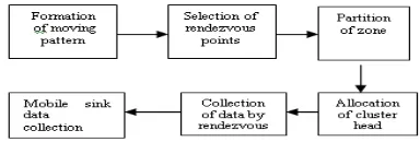
[image:2.612.85.277.660.725.2]Figure 1. Shows the steps to be implemented for the tour formation. First the moving pattern is being formed. The nearest node is being selected as RP and sensor nodes which is being selected forward the data to mobile sink. The area is being divided into zone. The cluster head is allocated. Thus the data is being transferred to WRP. Weight is assigned to each rendezvous, so that the mobile sink travel along the path to collect the data.
Figure-1. Steps implemented for tour formation.
a) Weighted rendezvous planning
WRP preferentially designates sensor nodes with the highest weight as a RP. The weight of a sensor node is calculated by multiplying the number of packets that it forwards by its hop distance to the closest RP on the tour. Thus, the weight of sensor node ‘i’ is calculated as
Wi = NFD(i) × H(i, M).
NFD(i) = no of packet send by node. H(i, M) = hop distance of node from
rendezvous.
Sensor nodes that are one hop away from an RP and have one data packet buffered get the minimum weight. Hence, sensor nodes that is farther away from the selected RPs or has more than one packet in their buffer have a higher priority of being recruited as an RP.
Mobile sink collect the data from RPs so that the delay and energy consumption is minimized. The usage of energy will take place even when the sensor node is idle. But the usage of energy will be more when the sensor node transmit or when the sensor node is received.
b) Cluster
Clustering is the efficient method to improve the lifetime of the network. Energy efficient clustering scheme is used because it can interact with each sensor through the localized communication, it can balance the load among the cluster head. The cluster head is the one which is having highest energy. The communication is done by single hop to WRP. The cluster head is being changed periodically inorder to prevent the formation of energy holes.
c) Performance evaluation
The events are traced by using the trace files in simulation time. The trace files is executed based on the performance evaluated in the network. Into trace files the events are recorded while record procedure executed. We trace the events like Packets lost, received packet in record procedure, received time of last packet etc. The trace file has the trace values written into it. This procedure called for every 0.05 ms is recursively. So for every 0.05 ms the trace value is recorded.
4. SOFTWARE SIMULATION
a) Implementation in NS2
NAM) and to analyze (using Xgraph/GNUplot) the simulation results are presented.
Network Simulator (NS), a discrete event simulator targeted at networking research is widely used by researchers in universities and companies. For simulation of routing, TCP and multicast protocols over wireless and wired (local and satellite) networks, NS provides substantial support. The latest version of NS is 2.26 (NS2). It implements network protocols such as Telnet and FTP, SPF and DV which is routing algorithms, and 'lower' layers such as logic link (LL) and media access control (MAC). NS began as a variant of the REAL network simulator in 1989. In 1995 NS development was supported by DARPA through the VINT project at Xerox PARC, LBL, USC/ISI and UCB. NS development currently support through DARPA with SAMAN and through NSF with CONSER. NS has always included substantial contributions from other researchers, including UCB, ACIRI, Sun Microsystems and CMU.
Nam began at LBL. The Nam development effort was an on going collaboration with the project named VINT. Currently, it is being developed at ISI as part of the SAMAN and Sensor projects.
The simple way NS2 can be used is for studying the property of a well-known protocol. In this case, a script language OTcl is used to glue the network components (nodes, links, agents, applications, etc) provided by NS2, configure the parameters (band-width, delay, routing protocol, etc) and launch activities (data transfer, topology change, etc). In trace files NS2 will read these configurations; simulate each record event, statistics, network event. Nam can demonstrate the events in a visualized way only after the simulation. For the simple usage of NS2, an understanding to the simulation framework is necessary.
When NS2 is used to simulate a new protocol, e.g., an ad hoc wireless routing protocol, the simple way is not enough. The advanced way is to hack the source of NS2 with C++, define new network components, rebuild the whole system and run the customized version of NS2.
Figure-2. Operation of output screen.
NS2 simulation is about the processing of packets. Packets are transported among network nodes via
network links. These packets are generated by network applications (data packet) or network protocols (control packet). Figure-4.1 shows the operation of output screen.
An event scheduler is in charge of ordering all the packets (or events) by their arriving time and let nodes, links and agents to handle these packets in sequence. A full trace of each packet or their statistics information can be stored in a trace file, and used to generate graphs or animations. In this section, the concept of node, link, agent, and scheduler will be introduced, as well as their usage in an OTcl script to configure a specific NS2 simulation.
5. RESULTS AND DISCUSSIONS
Figure-3. Transformation of data.
Figure-3 shows division of zone. There are 47 nodes and has four zone. The zone division is represented by four colours such as orange, red, green, brown. The pink circle denotes the rendezvous points. The blue colour denotes the sink nodes.The mobile sink travel along the path to collect the data. The highest weight will be given first preferrance and mobile sink collects the data from it.
The highest energy is considered as the cluster head. From the cluster head the data is being transferred to Weighted Rendezvous Planning. Then the mobile travel along the path to collect the data from it. Because of Energy Efficient Clustering Scheme the network lifetime is being improved and delay is also being reduced.
Figure-4. Shows the simulation graph for energy.X-axis denotes the time and Y-axis denotes energy. The green colour line represent the energy level by using the cluster. The Red colour line in the graph indicates energy level by using Weighted Rendezvous Planning. Thus from the above graph it is clear that residual energy using cluster is efficient when compared to Weighted Rendezvous Planning.
Figure-5(a). The simulation graph for throughput.
The throughput gives packet delivery ratio. The green colour line represent the throughput using cluster. The red colour line represent the throughput using Weighted Rendezvous Planning.Thus from above graph it is clear that using cluster is efficient method. X-axis denotes time, Y-axis denotes number of packets as shown in Figure-5.The throughput of a communication system may be affected by factors like available processing power of the end user behavior and system components.
When various protocol overheads are taken into account, the transferred data at useful rate can be significantly lower than the maximum achievable throughput. The rate of successful message delivery over communication channel. The throughput increased.
Figure-5(b). Simulation graph for packet received.
Figure-5. Simulation graph for packet received. X-axis shows time, Y-axis denotes packets. The packet dropping may occur due to collisions, buffer overflows, congestion, etc. From the the above graph it is clear that the packet received using cluster is efficient when compared to Weighted Rendezvous Planning.
Figure-6. The simulation graph for delay.
Figure-6 shows the simulation graph for delay. X-axis denotes simulation time. Y-axis denotes weighting time. The red colour line indicates delay by using weighted rendezvous planning. The green colour line indicates delay by using the clustereing. From the above graph it is clear that delay is being reduced by using cluster when compared to weighted rendezvous planning.
Delay varies with time .It occurs due to traffic and congestion. In sensor network data should not be dropped during the transmission and it should be guaranteed not to exceed a maximum worst-case delay.
6. CONCLUSIONS
Thus inside the zone, cluster operation is done. In each region, one cluster head is selected from the members of it by election based on energy level, so that other nodes can communicate with the cluster head. All the cluster head collecting data from cluster member send data to Weighted Rendezvous Points (RPs). From the Rendezvous Points (RPs) depend on the tour plan, mobile sink collects the data. Thus proposed work mainly deals with the how the usage of the cluster along with Weighted Rendezvous Planning is more efficient. Thus network lifetime is improved by reducing the delay, the packet received and throughput is also being improved.
REFERENCES
[1] I. F. Akyildiz, E. Cayirc, W. Su and Y. Sankara subramaniam. 2002. “Wireless sensor network: A survey,” Comput. Netw., pp. 393–422. Vol. 38, no. 4, March.
integration,” in Proc. 5th IEEE Int. Conf. Ind. Inform., Vienna, Austria, pp. 317–322. Vol. 1, June.
[3] A. Mainwaring, D. Culler, R. Szewczyk, J. Polastre and J. Anderson. 2002. “Wireless sensor networks for habitat monitoring,” in proc.1st ACM Int. Workshop Wireless Sensor Network September. pp. 88–97.
[4] J. Kamimura, et. al. 2004. Energy-E±cient Cluster-ing Method for Data Gathering in Sensor Net-works," in the Annual International Conference on Broadband Networks, October.
[5] Z. Yin, J. Zhang, S. Liu, W. Li, S. Liu and X. Guo. 2009. “Forest fire detection system based on wireless sensor network,” In: IEEE Conf. Ind. Electron. Appl., Xi’an, China, pp. 520–523, May.
[6] L. Lunadei, L. Ruiz-Garcia, I. Robla and P. Barreiro. 2009. “A review of wireless sensor technologies and applications in agriculture and food industry .State of the current trends and art,” Sensors, no. 6, Vol. 9, June.
[7] N. Wang, M. Wang and N. Zhang. 2006. “Wireless sensors in agriculture, food industry–recent development and future perspective,” Comput. Electron. Agriculture, pp. 1-14, Vol. 50, no.1, January.
[8] A. Wheeler. 2007. “Commercial applications of wireless sensor networks using zigbee,” IEEE Commun. pp. 70-77. Vol. 45, Mag. no 4, April.
[9] W. Chen, L. Chen, S. Tu and Z. and Chen S. 2006. “Wits: A wireless sensor network for intelligent transportation system,” in Proc. 1st Int. Multi-Symp. Comput. Comput. Sci., Hangzhou, China, Jun. Vol. 2, pp. 635–641.
[10] S. Lindsey, et al. 2002. PEGASIS: Power-Efficient Gathering in Sensor Systems," IEEE Aerospace Conference Proceedings , pp. 1125-1130, Vol. 3, 9-16.
[11] M. Ye, G. Chen, C. Li and J. Wu. 2007. “An unequal cluster based Routing protocol in wireless sensornet works,” Wireless ,Networks, pp. 193–207 April.
[12]A. A. Abbasi and M. Younis. 2007. “A survey on clustering algorithms for wireless sensor networks,” Computer. Vol. 30, pp. 2826–2841.
[13] W. B. Heinzelman and S. Soro. 2005. “Prolonging lifetime of wireless sensor networks via unequal clustering,” in IPDPS.
[14] I. Bekmezci and F. Alagz. 2009. “Energy efficient,