Technical note: Towards a continuous classification of climate using bivariate colour mapping

www.hydrol-earth-syst-sci.net/15/3071/2011/ doi:10.5194/hess-15-3071-2011

© Author(s) 2011. CC Attribution 3.0 License.

Earth System

Sciences

Technical note: Towards a continuous classification of climate using

bivariate colour mapping

A. J. Teuling

Hydrology and Quantitative Water Management Group, Wageningen University, The Netherlands Received: 29 April 2011 – Published in Hydrol. Earth Syst. Sci. Discuss.: 17 June 2011

Revised: 2 September 2011 – Accepted: 4 October 2011 – Published: 7 October 2011

Abstract. Climate is often defined in terms of discrete classes. Here I use bivariate colour mapping to show that the global distribution of K¨oppen-Geiger climate classes can largely be reproduced by combining the simple means of two key states of the climate system (i.e. air temperature and rela-tive humidity). This allows for a classification that is not only continuous in space, but can be applied at and transferred be-tween timescales ranging from days to decades.

1 Introduction

According to a popular phrase, we are told that “climate is what you expect, weather is what you get”. Climate is thus defined as the weather averaged over a long period of time, usually 30 yr. Ideally, one would therefore rigorously de-fine climate based on expected (i.e. mean) values of climate variablesXi only:

Climate type=f (E[X1],E[X2],...). (1)

Such a definition can be applied at any temporal (and spa-tial) scale ranging from minutes (providedXi is a continu-ous variable) to decades and could link short-term climate realizations and extremes to average conditions in that re-gion or elsewhere. Here, I will explore the potential of such a classification.

Current classification systems are often scale-invariant and explicitly define their resolution in time and space (i.e. through a limited number of classes). The widely

Correspondence to: A. J. Teuling ([email protected])

used K¨oppen-Geiger system (K¨oppen, 1884, 1918), for stance, has a pre-defined number of classes and utilizes in-formation on long-term averages on both yearly and monthly timescales. As a result, the K¨oppen-Geiger system accounts for effects of seasonality but variations on other timescales that are relevant to climate and ecosystem functioning are ignored (e.g. diurnal temperature range, decadal variations, El Ni˜no). Discrete climate classes imply that changes in the distribution of climate zones can only be detected along cli-mate class edges (for examples see Kim et al., 2008; Rubel and Kottek, 2010). In addition, the K¨oppen-Geiger system mixes statistics of a continuous atmospheric state (air tem-perature) and a discontinuous flux field with stochastic prop-erties (precipitation). And while the K¨oppen-classification has been derived manually to predict vegetation patterns rather than climate itself, it does not make optimal use of the information contained in the meteorological observa-tions (Cannon, 2011).

2 Towards spatial continuity

Considering these disadvantages, it is clear that the earth sys-tem and climate sciences community could benefit from a spatially continuous and conceptually more consistent classi-fication of climate. It is also clear that any climate classifica-tion should at least contain measures of temperature (T) and water availability. Rather than the amount of water that infil-trates into the soil or runs off during intermittent rain events (as in the K¨oppen classification) or that is stored in the soil (as in the Thornthwaite classification), I use screen-level rel-ative humidity (RH) as a robust and well-defined measure of water availability in the environment:

3072 A. J. Teuling: Continuous climate classification

30 40 50 60 70 80 90

−50 −40 −30 −20 −10 0 10 20 30 Af Am As Aw BSh BSk BWh BWk Cfa Cfb Cfc Csa Csb Csc Cwa Cwb Cwc Dfa Dfb Dfc Dfd Dsa Dsb Dsc Dwa Dwb Dwc Dwd EF ET

Relative humidity (%)

Temperature (

° C)

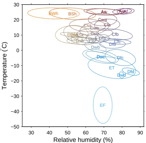
Fig. 1. Distribution of the K¨oppen-Geiger climate classes in theT, RH-space. Contours are fitted bivariate Gaussian densities provid-ing a measure of the spread within each class.

Note that bothT and RH are continuous variables defined for any time interval. For my analysis, I use gridded observations (10 min spatial resolution resampled to 0.5 degree resolution) for the period 1961–1990 compiled by the Climate Research Unit (e.g. New et al., 2002; Mitchell and Jones, 2005), and the K¨oppen-Geiger climate classification for the same period at 0.5 degree resolution as derived by Kottek et al. (2006).

Indeed, RH separates grid cells with classes that have sim-ilar average temperature but different rainfall characteristics, such as BWh, BSh, As/Aw and Am/Af (Fig. 1). Similarly, the different C, D, and E classes show a preference for a par-ticular subspace. Note that the dependency of the K¨oppen classes on RH is indirect since the link between the amount of rain during discrete rain events used in the K¨oppen clas-sification and the yearly average RH depends also on the re-evaporation of rainwater into the atmosphere.

While conceptually straightforward, visualization of such classification requires bothT and RH to be plotted simul-taneously. This can be achieved by a technique called bi-variate colour mapping, in which every colour on the map corresponds not to a single value of a variable as in conven-tional colour mapping, but rather to a unique combination of two variables. Bivariate colour mapping can be an effec-tive method to display how fields of two different variables co-vary in space. Examples of the application of bivariate colour maps to earth system sciences can be found in Albani et al. (2006), Teuling et al. (2009), and Miralles et al. (2011). For more information on bivariate colour mapping and con-struction of colour legends I refer to Teuling et al. (2011).

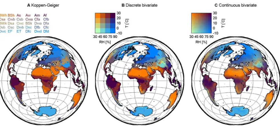
Figure 2a shows the current distribution of climate accord-ing to the K¨oppen-Geiger classification as derived by Kottek et al. (2006). The colour for each climate class is selected based on its mean position in theT, RH-space (Fig. 1). In this way, the global patterns can be directly compared to a map in which distribution of mean temperature and relative humidity have been plotted using bivariate colour mapping with a limited number of colours (Fig. 2b). The number of colours (4×4) has been chosen such that upon visual inspec-tion the class boundaries roughly align with those in Fig. 2a. However, no optimization has been performed, the classes are equally-spaced in theT- and RH-space, and the resulting number of classes or colors (16) is different from the number in the K¨oppen-Geiger classification.

In spite of these limitations, the resulting maps are sur-prisingly similar, indicating that in addition to temperature, the yearly average rainfall as well as its seasonal distribution are reflected in the average relative humidity. Not only are the boundaries along wet-dry and warm-cold transitions well captured, even complex gradients, such as the combination of a north-south temperature gradient with a east-west hu-midity gradient in North-America, are captured. Differences occur over the Tibetan plateau, where the low humidity com-pared to regions with similar temperature is not reflected in the K¨oppen-Geiger map. Thus, by combining average tem-perature and relative humidity, the same global climate pat-terns emerge as those obtained by the much more complex K¨oppen-Geiger classification.

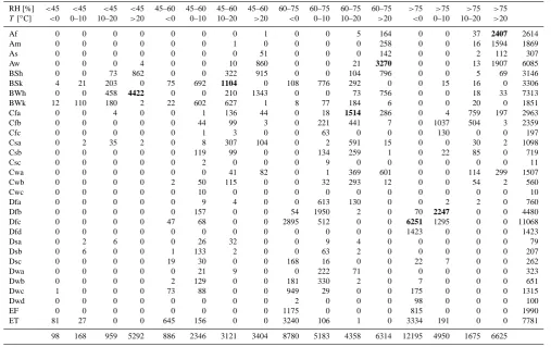
It should be noted, however, that these maps cannot read-ily be compared in a quantitative manner since this would re-quire the difference between two colours (with 3 degrees of freedom) to be expressed in a single number. Also, the match between the two patterns depends on the (arbitrary) resolu-tion in RH andT. An alternative quantitative comparison is provided in Table 1, where the number of overlapping cells between the K¨oppen-Geiger (Fig. 2a) and bivariate (Fig. 2b) classifications are listed. There is a good correspondence in patterns, in particular for the climate classes that span a wider range in temperature and humidity (bold values in Table 1) roughly corresponding to the 4×4 division in RH andT. To improve the correspondence with classes that span a smaller range in RH andT, a finer division in RH andT would be needed; see also the evaluation of the K¨oppen-Geiger classes in theT, RH-space provided by Fig. 1.

Fig. 2. Global distribution of climate zones. (A): K¨oppen-Geiger classification. Colouring is taken from Fig. 1. Data are taken from Kottek et al. (2006). (B): Discrete (4×4) bivariate classification of climate based on expected values ofT and RH. (C): (Near-)continuous (16×16) bivariate classification. Note the correspondence between (A) and (B). Data in (A) and (B) are gridded observations (10 min spatial resolution resampled to 0.5 degree resolution) for the period 1961–1990 compiled by the Climate Research Unit (e.g. New et al., 2002; Mitchell and Jones, 2005) extended with ERA-40 reanalysis over the Antarctic.

20 40 60 80 100 −10

0 10 20 30

Relative humidity (%)

Temperature (

° C)

A De Bilt

20 40 60 80 100 −10

0 10 20 30

Relative humidity (%) B Madrid

Fig. 3. Daily average temperature and relative humidity over the recent period 2001–2010 at De Bilt (A) and Madrid (B). Contour lines indicate the shape of the density maxima for the complete cli-mate record. Crosses indicate mean values of RH andT. Observa-tions are taken from the European Climate Assessment & Dataset (ecad.knmi.nl).

3 Linking weather and climate

Next, I illustrate how colour can be used to visually link near-surface atmospheric conditions at different timescales. Figure 3 shows the distribution of long-term observations of daily averageT and RH at two European stations with dif-ferent seasonal climate dynamics: De Bilt (The Netherlands, Cfb climate) and Madrid (Spain, Csa climate), for which data is available via the European Climate Assessment & Dataset

(ecad.knmi.nl). The individual days are plotted using the same colours as in Fig. 1. By doing so, the weather on one particular day (as characterized by the color that combines its T and RH) can be directly linked to average climate condi-tions in those regions in Fig. 2c that have the same colour. Al-ternatively, it could be linked to a bivariate colour map show-ing the expected values ofT and RH for that particular day.

It can be seen that on a daily timescale, weather condi-tions can vary over a range ofT and RH that cover the av-erage conditions for most climate classes (see Fig. 1). Dur-ing warm and dry summer conditions, air masses over The Netherlands often originate from the Sahara, and the orange colours indicate temperature and relative humidity typical for BWh climates. During cold extremes in winter, air masses typically have arctic origin and the light-blue colours indi-cate that these conditions correspond to average conditions for a Dfc climate. It should be noted that local processes can also have an important impact on temperature extremes in Europe, as was shown by Fischer et al. (2007) for warm ex-tremes. Also note that seasonality induces preffered summer and winter states in the bivariate distribution ofT and RH.

3074 A. J. Teuling: Continuous climate classification

Table 1. Correspondence between Fig. 2a and b expressed by the number of 0.5 degree cells overlapping each class in the K¨oppen-Geiger and bivariate classification. The last row and column represent the total sum for each classification class. Note that these numbers are not optimized values since the number of bivariate classes (16) and the temperature and relative humidity limits are chosen arbitrary. Bold values indicate which value is largest for each row and column simultaneously. Antarctica is omitted from the analysis.

RH [%] <45 <45 <45 <45 45–60 45–60 45–60 45–60 60–75 60–75 60–75 60–75 >75 >75 >75 >75

T[◦_{C] <0 0–10 10–20 >20 <0 0–10 10–20 >20 <0 0–10 10–20 >20 <0 0–10 10–20 >20}

Af 0 0 0 0 0 0 0 1 0 0 5 164 0 0 37 2407 2614

Am 0 0 0 0 0 0 1 0 0 0 0 258 0 0 16 1594 1869

As 0 0 0 0 0 0 0 51 0 0 0 142 0 0 2 112 307

Aw 0 0 0 4 0 0 10 860 0 0 21 3270 0 0 13 1907 6085

BSh 0 0 73 862 0 0 322 915 0 0 104 796 0 0 5 69 3146

BSk 4 21 203 0 75 692 1104 0 108 776 292 0 0 15 16 0 3306

BWh 0 0 458 4422 0 0 210 1343 0 0 73 756 0 0 18 33 7313

BWk 12 110 180 2 22 602 627 1 8 77 184 6 0 0 20 0 1851

Cfa 0 0 4 0 0 1 136 44 0 18 1514 286 0 4 759 197 2963

Cfb 0 0 0 0 0 44 99 3 0 221 441 7 0 1037 504 3 2359

Cfc 0 0 0 0 0 1 3 0 0 63 0 0 0 130 0 0 197

Csa 0 2 35 2 0 8 307 104 0 2 591 15 0 0 30 2 1098

Csb 0 0 0 0 0 119 99 0 0 134 259 1 0 22 85 0 719

Csc 0 0 0 0 0 2 0 0 0 9 0 0 0 0 0 0 11

Cwa 0 0 0 0 0 0 41 82 0 1 369 601 0 0 114 299 1507

Cwb 0 0 0 0 2 50 115 0 0 32 293 12 0 0 54 2 560

Cwc 0 0 0 0 0 10 0 0 0 0 0 0 0 0 0 0 10

Dfa 0 0 0 0 0 9 4 0 0 613 130 0 0 2 2 0 760

Dfb 0 0 0 0 0 157 0 0 54 1950 2 0 70 2247 0 0 4480

Dfc 0 0 0 0 47 68 0 0 2895 512 0 0 6251 1295 0 0 11068

Dfd 0 0 0 0 0 0 0 0 0 0 0 0 1423 0 0 0 1423

Dsa 0 2 6 0 0 26 32 0 0 9 4 0 0 0 0 0 79

Dsb 0 6 0 0 1 133 2 0 0 63 2 0 0 0 0 0 207

Dsc 0 0 0 0 19 30 0 0 168 16 0 0 22 7 0 0 262

Dwa 0 0 0 0 0 21 9 0 0 222 71 0 0 0 0 0 323

Dwb 0 0 0 0 2 129 0 0 181 330 2 0 7 0 0 0 651

Dwc 1 0 0 0 73 88 0 0 949 29 0 0 175 0 0 0 1315

Dwd 0 0 0 0 0 0 0 0 2 0 0 0 98 0 0 0 100

EF 0 0 0 0 0 0 0 0 1175 0 0 0 815 0 0 0 1990

ET 81 27 0 0 645 156 0 0 3240 106 1 0 3334 191 0 0 7781

98 168 959 5292 886 2346 3121 3404 8780 5183 4358 6314 12195 4950 1675 6625

4 Conclusions

In summary, by linking combinations of two spatially and temporally continuous fields (air temperature and relative humidity) to unique colours, a straightforward and easy-to-understand approximation of the distribution of global climate zones can be obtained. An important advantage of this method is that the continuous nature of the variables result in temporal means that are well-defined and meaningful at any time resolution. The proposed method can thus be used to bridge the gap between the weather that you get on any particular day, and the climate you expect at that location, or at any place on Earth.

Acknowledgements. I acknowledge financial support from The Netherlands Organisation for Scientific Research through Veni Grant 016.111.002.

Edited by: R. Woods and H. H. G. Savenije

References

Albani, M., Medvigy, D., Hurtt, G. C., and Moorcroft, P. R.: The contributions of land-use change, CO2fertilization, and climate variability to the Eastern US carbon sink. Glob. Change Biol. 12, 2370–2390, 2006.

Cannon, A. J.: K¨oppen versus the computer: an objective com-parison between the K¨oppen-Geiger climate classification and a multivariate regression tree, Hydrol. Earth Syst. Sci. Discuss., 8, 2345–2372, doi:10.5194/hessd-8-2345-2011, 2011.

Fischer, E. M., Seneviratne, S. I., L¨uthi, D., and Sch¨ar, C.: Contribution of land-atmosphere coupling to recent Euro-pean summer heat waves, Geophys. Res. Lett., 34, L06707, doi:10.1029/2006GL029068, 2007.

Kim, H. J., Wang, B., Ding, Q. H., and Chung, I. U.: Changes in arid climate over North China detected by the Koppen climate classification, J. Meteorol. Soc. Jpn., 86, 981–990, 2008. K¨oppen, W.: Die W¨armezonen der Erde, nach der Dauer der

and Br¨onnimann, S., Meteorol. Z. 20, 351–360, 2011). K¨oppen, W.: Klassifikation der Klimate nach Temperatur,

Nieder-schlag und Jahresablauf (Classification of climates according to temperature, precipitation and seasonal cycle), Petermanns Ge-ogr. Mitt. 64, 193–203, 243–248, 1918.

Kottek, M., Grieser, J., Beck, C., Rudolf, B., and Rubel, F.: World map of the K¨oppen-Geiger climate classification updated, Mete-orol. Z., 15, 259–263, doi:10.1127/0941-2948/2006/0130, 2006. Miralles, D. G., De Jeu, R. A. M., Gash, J. H., Holmes, T. R. H., and Dolman, A. J.: Magnitude and variability of land evaporation and its components at the global scale, Hydrol. Earth Syst. Sci., 15, 967–981, doi:10.5194/hess-15-967-2011, 2011.

Mitchell, T. D., and Jones, P. D.: An improved method of con-structing a database of monthly climate observations and as-sociated high-resolution grids, Int. J. Climatol., 25, 693–712, doi:10.1002/joc.1181, 2005.

New, M., Lister, D., Hulme, M., and Makin, I.: A high resolution data set of surface climate over global land areas, Clim. Res., 21, 1–25, 2002.

Rubel, F. and Kottek, M.: Observed and projected climate shifts 1901–2100 depicted by world maps of the K¨oppen-Geiger climate classification, Meteorol. Z., 19, 135–141, doi:10.1127/0941-2948/2010/0430, 2010.

Teuling, A. J., Hirschi, M., Ohmura, A., Wild, M., Reichstein, M., Ciais, P., Buchmann, N., Ammann, C., Montagnani, L., Richard-son, A. D., Wohlfahrt, G., and Seneviratne, S. I.: A regional perspective on trends in continental evaporation, Geophys. Res. Lett., 36, L02404, doi:10.1029/2008GL036584, 2009.