Simulation of rainfall time series from different climatic regions using the direct sampling technique

www.hydrol-earth-syst-sci.net/18/3015/2014/ doi:10.5194/hess-18-3015-2014

© Author(s) 2014. CC Attribution 3.0 License.

Simulation of rainfall time series from different climatic regions

using the direct sampling technique

F. Oriani1, J. Straubhaar1, P. Renard1, and G. Mariethoz2

1_{Centre for Hydrogeology and Geothermics, University of Neuchâtel, Neuchâtel, Switzerland}

2_{School of Civil and Environmental Engineering, University of New South Wales, Sydney, New South Wales, Australia} Correspondence to: F. Oriani ([email protected])

Received: 21 February 2014 – Published in Hydrol. Earth Syst. Sci. Discuss.: 21 March 2014 Revised: 30 June 2014 – Accepted: 2 July 2014 – Published: 14 August 2014

Abstract. The direct sampling technique, belonging to the family of multiple-point statistics, is proposed as a nonpara-metric alternative to the classical autoregressive and Markov-chain-based models for daily rainfall time-series simulation. The algorithm makes use of the patterns contained inside the training image (the past rainfall record) to reproduce the complexity of the signal without inferring its prior statistical model: the time series is simulated by sampling the train-ing data set where a sufficiently similar neighborhood exists. The advantage of this approach is the capability of simulat-ing complex statistical relations by respectsimulat-ing the similarity of the patterns at different scales. The technique is applied to daily rainfall records from different climate settings, using a standard setup and without performing any optimization of the parameters. The results show that the overall statis-tics as well as the dry/wet spells patterns are simulated ac-curately. Also the extremes at the higher temporal scale are reproduced adequately, reducing the well known problem of overdispersion.

1 Introduction

The stochastic generation of rainfall time series is a key topic for hydrological and climate science applications: the challenge is to simulate a synthetic signal honoring the high-order statistics observed in the historical record, re-specting the seasonality and persistence from the daily to the higher temporal scales. Among the different proposed techniques, exhaustively reviewed by Sharma and Mehrotra (2010), the most commonly adopted approach to the problem

since the 1960s is the Markov-chain (MC) simulation: in its classical form, it is a linear model which cannot simu-late the variability and persistence at different scales. So-lutions to deal with this limitation consist of introducing exogenous climatic variables and large-scale circulation in-dexes (Hay et al., 1991; Bardossy and Plate, 1992; Katz and Parlange, 1993; Woolhiser et al., 1993; Hughes and Guttorp, 1994; Wallis and Griffiths, 1997; Wilby, 1998; Kiely et al., 1998; Hughes et al., 1999), lower-frequency daily rainfall co-variates (Wilks, 1989; Briggs and Wilks, 1996; Jones and Thornton, 1997; Katz and Zheng, 1999) or an index based on the short-term daily historical or previously generated record (Harrold et al., 2003a, b; Mehrotra and Sharma, 2007a; Mehrotra and Sharma, 2007b) as conditioning variables for the estimation of the MC parameters. By doing this, nonlin-earity is introduced in the prior model, and the MC param-eters change with time as a function of some specific low-frequency fluctuations. An alternative method proposed is model nesting (Wang and Nathan, 2002; Srikanthan, 2004, 2005; Srikanthan and Pegram, 2009), which implies the cor-rection of the generated daily rainfall using a multiplicative factor to compensate the bias in the higher-scale statistics. These techniques generally allow a better reproduction of the statistics up to the annual scale, but they imply the estimation of a more complex prior model and cannot completely cap-ture a complex dependence struccap-ture.

developed during the last decade (Strebelle, 2002; Allard et al., 2006; Zhang et al., 2006; Arpat and Caers, 2007; Honarkhah and Caers, 2010; Straubhaar et al., 2011; Tah-masebi et al., 2012), MPS is a family of geostatistical tech-niques widely used in spatial-data simulations and particu-larly suited to pattern reproduction. MPS algorithms use a training image; i.e., a data set to evaluate the probability dis-tribution (pdf) of the variable simulated at each point (in time or space), conditionally to the values present in its neighbor-hood. In the particular case of the DS technique, the con-cept of training image is taken to the limit by avoiding the computation of the conditional pdf and making a random sampling of the historical data set where a pattern similar to the conditioning data is found. If the training data set is representative enough, these techniques can easily reproduce high-order statistics of complex natural processes at different scales. MPS has already been successfully applied to the sim-ulation of spatial rainfall occurrence patterns (Wojcik et al., 2009). In this paper, we test the DS technique on the simula-tion of daily rainfall time series. The aim is to reproduce the complexity of the rainfall signal up to the decennial scale, simulating the occurrence and the amount at the same time with the aid of a multivariate data set. Similar algorithms per-forming a multivariate simulation had been previously de-veloped by Young (1994) and Rajagopalan and Lall (1999) using a bootstrap-based approach. As discussed in detail in Sect. 2.3, the advantage of DS with respect to the mentioned techniques is the possibility to have a variable high-order time-dependence, without incurring excessive computation since the estimation of then-dimensional conditional pdf is not needed. Moreover, we propose a standard setup for rain-fall simulation: an ensemble of auxiliary variables and fixed values for the main parameters required by the direct sam-pling algorithm, suitable for the simulation of any stationary rainfall time series, without the need of calibration. The tech-nique is tested on three time series from different climatic regions of Australia. The paper is organized as follows: in Sect. 2 the DS algorithm is introduced and compared with the existing resampling techniques. The data set used, the proposed setup and the method of evaluation are described in Sect. 3. The statistical analysis of the simulated time series is presented and discussed in Sect. 4 and Sect. 5 is dedicated to the conclusions.

2 Methodology

In this section we recall the basics of multiple-point statistics and we focus on the direct sampling algorithm. The data set used is then presented as well as the methods of evaluation. 2.1 Background on multiple-point statistics

Before entering in the details of the DS algorithm, let us introduce some common elements of MPS. The whole

information used by MPS to simulate a certain process is based on the training image (TI) or training data set: the data set constituted of one or more variables used to infer the statistical relations and occurrence probability of any datum in the simulation. The TI may be constituted of a concep-tual model instead of real data, but in the case of the rainfall time series it is more likely to be a historical record of rainfall measurements. The simulation grid (SG) is a time-referenced vector in which the generated values are stored during the simulation. Following a simulation path which is usually ran-dom, the SG is progressively filled with simulated values and becomes the actual output of the simulation. The con-ditioning data are a group of given data (e.g., rainfall mea-surements) situated in the SG. Being already informed, no simulation occurs at those time steps. The presence of con-ditioning data affects, in their neighborhood, the conditional law used for the simulation and limits the range of possible patterns. MPS, as well some MC-based algorithms for rain-fall simulation (see Sect. 1), may include the use of auxiliary variables to condition the simulation of the target variable. Auxiliary variables may either be known (fully or partially) and used to guide the simulation, or they may be unknown but still cosimulated because their structures contain impor-tant characteristics of the signal. For rainfall time series it could be, for example, covariates of the original or previously simulated data (e.g., the number of wet days in a past period), a correlated variable for which the record is known, a theo-retical variable that imposes a periodicity or a trend (e.g., a sinusoid function describing the annual seasonality over the data). Finally, the search neighborhood is a moving window – i.e., the portion of time series located in the past and future neighborhood of each simulated value – used to retrieve the data event; i.e., the group of time-referenced values used to condition the simulation.

2.2 The direct sampling algorithm

Classical MPS implementations create a catalog of the possi-ble neighbor patterns to evaluate the conditional probability of occurrence for each event with respect to the considered neighborhood. This may imply a significant amount of mem-ory and always limits the application to categorical variables. On the contrary, the DS algorithm generates each value by sampling the data from the TI where a sufficiently similar neighborhood exists. The DS implementation used in this pa-per is called DeeSse (Straubhaar, 2011). The following is the main workflow of the algorithm for the simulation of a single variable. For the multivariate case see the last paragraph of this section.

Let us denotex=[x1, . . . ,xn] the time vector represent-ing the SG,y=[y1, . . . ,ym] the one representing the TI and

Z(·)the target variable, object of the simulation, defined at each element ofx andy. Before the simulation begins, all continuous variables are normalized using the transformation

(see step 3) in the range [0, 1]. During the simulation, the un-informed time steps of the SG are visited in a random order. The random simulation patht∈ {1,2, . . . , M}is obtained by sampling without replacement the discrete uniform distribu-tionU (1, M)whereMis the SG length. At each uninformed

xt, the following steps are executed:

1. The data eventd(xt)= {Z(xt+h1), . . . , Z(xt+hn)}is

re-trieved from the SG according to a fixed neighborhood of radiusRcentered onxt. It consists of at mostN in-formed time steps, closest to xt. This defines a set of lags H= {h1, . . . , hn}, with |hi| ≤R andn≤N. The size ofd(xt)is therefore limited by the user-defined pa-rameterN and the available informed time steps inside the search neighborhood.

2. A random time step yi in y is visited and the corre-sponding data event d(yi), defined according toH, is retrieved to be compared withd(xt).

3. A distance D(d(xt), d(yi)) – i.e., a measure of dis-similarity between the two data events – is calculated. For categorical variables (e.g., the dry/wet rainfall se-quence), it is given by the formula

D (d(xt) ,d(yi))= 1

n

n X

j=1

aj,

aj=

1 if Z xj6=Z yj 0 if Z xj=Z yj, (1) while for continuous variables the following one is used:

D (d(xt) ,d(yi))= 1

n

n X

j=1

|Z xj−Z yj|, (2)

where nis the number of elements of the data event. The elements ofd(xt), independently from their posi-tion, play an equivalent role in conditioning the simu-lation ofZ(xt). Note that, using the above distance for-mulas, the normalization is not needed for categorical variables, while for the continuous ones it ensures dis-tances in the range [0, 1].

4. If D(d(xt), d(yi)) is below a fixed threshold T – i.e., the two data events are sufficiently similar – the it-eration stops and the datumZ(yi)is assigned toZ(xt). Otherwise, the process is repeated from point 2 until a suitable candidate d(yi)is found or the prescribed TI fraction limitF is scanned.

5. If a TI fraction F has been scanned and the distance

D(d(xt), d(yi)) is above T for each visited yi, the datum Z(y_i∗) minimizing this distance is assigned to

Z(xt).

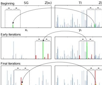
This procedure is repeated for the simulation at eachxt un-til the entire SG is covered. Figure 1 illustrates the iterative simulation using the DS technique and stresses some of its peculiarities. First, simulatingZ(xt) in a random order al-lowsxto be progressively populated at nonconsecutive time steps. Therefore, the simulation at eachxtcan be conditioned on both past and future, as opposed to the classical Markov-chain techniques, that use a linear simulation path starting from the beginning of the series, allowing conditioning on past only.

In the early iterations, the closest informed time steps used to condition the simulation are located far from xt and its number is limited by the search window; i.e., conditioning is mainly based on large past and future time lags. On the contrary, the final iterations dispose of a more populated SG, conditioning is thus done on small time lags since only the closestN values are considered. This variable time-lag prin-ciple may not respect the autocorrelation on a specific time lag rigorously, but it should preserve a more complex sta-tistical relationship, which cannot be explored exhaustively using a fixed-dependence model.

The DS can simulate multiple variables together similarly to the univariate case, dealing with a vector of variables Z(xt)and considering a data eventdkdifferent for eachkth variable, defined byNk andRk. Unlike the implementation presented in Mariethoz et al. (2010), DeeSse also uses a spe-cific acceptance threshold Tk for each variable. Step 3 of the algorithm is repeated until a candidate with a distance below the threshold for all variables is found. If this con-dition is not met, the scan stops at the prescribed TI frac-tionF and the error for each candidateyiandkth variable is computed with the following formula:Ek(yi)=(D(dk(xt), dk(yi))−Tk) T_k−1, whereD(·, ·)is defined as in step 3. Fi-nally, the candidate minimizing max(E(yi)) is assigned to Z(xt). Note that the entire data vectorZ(xt)is simulated in one iteration, reproducing exactly the same combination of values found for all the variables at the sampled time step, excluding the conditioning data, already present in the SG. This feature, although reducing the variability in the simula-tion, has been adopted to accurately reproduce the correlation between variables.

2.3 Comparison with existing resampling techniques

Beginning Z(x )t

xt

TI Z(y )t

yt SG

Final iterations Early iterations

Fig. 1. Sketch of the sequential simulation of a rainfall time-series performed by the Direct Sampling: the

dashed rectangle represents the search neighborhood of radius R, the datum being simulated is in green and the

ones composing the data event are in red. Note the non-exact match between the data event in the SG and the

one in the TI.

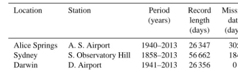
Table 1. Summary of the dataset used.

Location Station Period [years] Record length [days] Missing data [days]

Alice Springs A.S.Airport 1940-2013 26347 305

Sydney S.Observatory Hill 1858-2013 56662 184

Darwin D.Airport 1941-2013 26356 0

20

Figure 1. Sketch of the sequential simulation of a rainfall time series performed by the direct sampling technique: the dashed rectangle

represents the search neighborhood of radiusR, the datum being simulated is in green and the ones composing the data event are in red. Note the nonexact match between the data event in the SG and the one in the TI.

variance estimation, has seen several developments in hy-drology (Young, 1994; Lall and Sharma, 1996; Lall et al., 1996; Rajagopalan and Lall, 1999; Buishand and Brandsma, 2001; Wojcik and Buishand, 2003; Clark et al., 2004). Hav-ing different points in common with the DS technique, its general framework is briefly presented in the following. Each datum inside the historical record is characterized by a vector dt of predictor variables, analogous to the data event for DS. For example, to generateZ(xt)one could usedt=[Z(xt−1),

Z(xt−2,U (xt),U (xt−1)], meaning that the simulation is con-ditioned to the two previous time steps ofZand the present and previous time steps of U, a correlated variable. In the predictor variables space D, the historical data as well as

Z(xt), which still has to be generated, are represented as points whose coordinates are defined by dt. Consequently, proximity in Dcorresponds to similarity of the

condition-ing patterns. Z(xt)is simulated by sampling an empirical pdf constructed on thek points closest toZ(xt ); the closer the point is, the higher is the probability to sample the cor-responding historical datum. Proposed variations of the al-gorithm include transformations of the predictor variables space, the application of kernel smoothing to the k-NN pdf to increase the variability beyond the historical values, and different methods to estimate the parameters of the model; e.g.,kand the kernel bandwidth.

Going back to DS, the similarities with the k-NN bootstrap are that both (i) make a resampling of the historical record conditioned by an ensemble of auxiliary/predictor variables, and (ii) compute a distance as a measure of dissimilarity between the simulating time step and the candidates consid-ered for resampling. Nevertheless, there are several points of divergence in the rationale of the techniques: (i) in the k-NN bootstrap, the distance is used to evaluate the resam-pling probability, while in the DS it is used to evaluate the resampling possibility. This means that, using the k-NN re-sampling, the conditional pdf is a function of the distance, while in the DS the distance is only used to define its sup-port. In fact, using the DS, the spaceDis not restricted to

the k nearest neighbors but it is bounded by the distance thresholds: outside the boundary, the resampling probabil-ity is zero, while inside, it follows the occurrence of the data in the scanned TI fraction, without being a function of the pattern resemblance. Only in cases where no candidate is found, it is the closest neighbor outside the bounded portion ofDto be chosen for resampling. The latter can be

first datum presenting a distance below the threshold is sam-pled. This is an advantage since it avoids the problem of the high-dimensional conditional pdf estimation which limits the degree of conditioning in bootstrap techniques (Sharma and Mehrotra, 2010). (iii) The k-NN technique considers a fixed time-dependence, while it varies during the simulation in the case of DS. (iv) Finally, the simulation path (in the SG) is al-ways linear in the k-NN technique, while it is random using DS, allowing conditioning on future time steps of the target variable.

3 Application

The data set chosen for this study is composed of three daily rainfall time series from different climatic regions of Aus-tralia: Alice Springs (hot desert), with a very dry rainfall regime and long droughts, Sydney (temperate), with a far wetter climate due to its proximity to the ocean, and Darwin (tropical savannah), showing an extreme variability between the dry and wet seasons.

Table 1 presents the data set used: the chosen stations pro-vide a considerable record of about 70 years for Darwin and Alice Springs and 150 years for Sydney. Any gaps or trends have been explicitly kept to test the behavior of the algorithm with incomplete or nonstationary data sets. The direct sam-pling algorithm treats gaps in the time series in a simple way: each data event found in the TI is rejected if it contains any missing data. This allows incomplete training images to be dealt with in a safe way, but, as one could expect, a large quantity of missing data, especially if sparsely distributed, may lead to a poor simulation. Mariethoz and Renard (2010) show how DS can be used for data reconstruction.

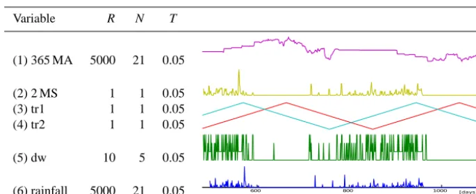
Since rainfall is a complex signal exhibiting not only mul-tiscale time-dependence but also intermittence, the classi-cal approach is to split the daily time-series generation in two steps: the occurrence model, where the dry/wet daily se-quence is generated using a Markov chain, and the amount model, where the rainfall amount is simulated on wet days using an estimation of the conditional pdf (e.g., Coe and Stern, 1982). The simulation framework proposed here is radically different: we use the direct sampling technique to generate the complete time series in one step, simulating multiple variables together. In particular, the TI used is based on the past daily rainfall record and composed of the follow-ing variables (Table 2): (1) the average rainfall amount on a 365-day centered moving window (365 MA; mm), (2) the moving sum of the current and the previous day amounts (2 MS; mm), (3) and (4) two out-of-phase triangular func-tions (tr1 and tr2) with frequency of 365.25 days, similar to trigonometric coordinates expressing the position of the day in the annual cycle, (5) the dry/wet sequence (i.e., a categori-cal variable indicating the position of a day inside the rainfall pattern: 1 – wet, 0 – dry, 2 – solitary wet, and 3 – wet day at the beginning or at the end of a wet spell), and (6) the daily

Table 1. Summary of the data set used.

Location Station Period Record Missing

(years) length data (days) (days)

Alice Springs A. S. Airport 1940–2013 26 347 305 Sydney S. Observatory Hill 1858–2013 56 662 184

Darwin D. Airport 1941–2013 26 356 0

rainfall amount, which is the target of the simulation. The first two auxiliary variables are covariates used to force the algorithm to preserve the interannual structure and the day-to-day correlation, which are known to exist a priori. The oth-ers are used to reproduce the dry/wet pattern and the annual seasonality accurately. Moreover, any unknown dependence in the daily rainfall signal is generically taken into account in the simulation by using a data event of variable length as ex-plained in Sect. 2.2. It has to be remarked that, apart from (3) and (4), which are known deterministic functions imposed as conditioning data, the rest of the auxiliary variables are trans-formations of the rainfall datum, automatically computed on the TI and cosimulated with the daily rainfall.

To summarize, the main parameters of the algorithm are the following: the maximum scanned TI fractionF∈(0, 1], the search neighborhood radiusR, the maximum number of neighborsN, both expressed in number of elements of the time vector, and the distance thresholdT∈(0, 1]. Recall that, apart fromF, each parameter is set independently for each simulated variable. The setup shown in Table 2 is used to-gether with F=0.5 and proposed as a standard for daily rainfall time series. A sensitivity analysis, not shown here, confirmed the generality of this setup which is not the result of a numerical optimization on a specific data set, but it is rather in accordance to the criteria used to define the order and extension of the variable time-dependence, as shown be-low. Applying it to any type of single-station daily rainfall data set, the user should obtain a reliable simulation without needing to change any parameter or give supplementary in-formation. An additional refinement of the setup is also pos-sible, keeping in mind the following general rules:

– Rlimits the maximum time-lag dependence in the sim-ulation and should be set according to the length of the largest sufficiently repeated structure or frequency in the signal that has to be reproduced. Being inter-ested to condition the simulation upon the inter-annual fluctuations (visible in the 10-year MA time series in Fig. 9), we setR365MS=Rrainfall=5000 for the 365 MS and daily rainfall variables. We recommend keepingR

Table 2. Standard setup proposed for rainfall simulation. The parameters are search window radiusR, maximum number of neighborsN

and distance thresholdT. The variables are (1) the 365-day moving average (365 MA), (2) the moving sum of the current and the previous day amounts (2 MS), (3) and (4) annual seasonality triangular functions (tr1 and tr2), (5) the dry/wet sequence (dw), and (6) the daily rainfall amount as the target variable. On the right, a portion of multivariate TI is given as example.

Variable R N T

(1) 365 MA 5000 21 0.05

(2) 2 MS 1 1 0.05 (3) tr1 1 1 0.05 (4) tr2 1 1 0.05

(5) dw 10 5 0.05

(6) rainfall 5000 21 0.05

distribution, in order to properly catch the continuity of the rainfall events over multiple days.

– N controls the complexity of the conditioning structure but also influences the specific time-lag dependence. For instance, if one increases N, higher-order depen-dencies are represented, but the weight accorded to a specific neighbor in evaluating the distance between patterns becomes lower. This leads to a less-accurate specific-time-lag conditioning, but a more complex time-dependence is respected on average. For the rain-fall amount and 365 MA variables,NRfollows the same setup rule as for Rdw. In this way, in the ini-tial iterations, the conditioning neighbors will be sparse in a 10 001-day window (R=5000) to respect low-frequency fluctuations, whereas, in the final iterations, they will be contained in a N-day window to respect the within-spell variability. The standard value pro-posed here (N365MA=N365MA=21) corresponds ap-proximately to the spell-distribution median of the Dar-win time series, remaining in the appropriate range for the other considered climates. Conversely,Ndw is kept lower in order to focus the conditioning on the small-scale dry/wet pattern.Ndw=5 gave in general the best result in terms of dry/wet pattern reproduction.

– For 2 MS, tr1 and tr2, the time-dependence is limited to lag 1 by usingN=R=1. This combination should not be changed since we have no interest in expanding or varying the time-lag dependence for the mentioned variables.

– T determines the tolerance in accepting a pattern. The sensitivity analysis done until now on different types of heterogeneities (Meerschman et al., 2013) con-firmed that the optimum generally lies in the interval [0.01, 0.07] (1–7 % of the total variation). HigherT val-ues usually lead to poorly simulated patterns, but lower

ones may induce a bias in the marginal distribution and increase the phenomenon of verbatim copy; i.e., the ex-act reproduction of an entire portion of data by oversam-pling the same pattern inside the TI. For these reasons, we recommend keeping the proposed standard value

T= 0.05 for all the variables.

– F should be set sufficiently high to have a consistent choice of patterns but a value close to 1 – i.e., all of the TI is scanned each time – may lower the variability of the simulations and increase the verbatim copy. Us-ing a trainUs-ing data set representative enough, the optimal value corresponds to a TI fraction containing some rep-etitions of the lowest-frequency fluctuation that should be reproduced. Considering the randomness of the TI scan, the valueF=0.5 chosen in this paper is sufficient to serve the purpose.

3.1 Imposing a trend

As already shown in Chugunova and Hu (2008), Mariethoz et al. (2010), Honarkhah and Caers (2010) and Hu et al. (2014), in case of a nonstationary target variable, the simula-tion can be constrained to reproduce the same type of trend found in the TI by making use of an auxiliary variable. The one proposed here is the integer vectorL=[1, 2, . . . ,M], whereMis the length of the time series, tracking the posi-tion of each datum inside the TI.Lis assigned to the SG as conditioning datum with the following parameters:RL=1,

same trend. The following remarks are noteworthy: (i) to avoid an unnecessary restriction of the sampling,TLshould correspond to the maximum time interval for which the tar-get variable can be considered stationary; (ii) the simulation should not be longer than the training data set, having no ba-sis to extrapolate the trend in the past or future; (iii) the local variability is not completely limited byL: a pattern outside the tolerance range (i.e., with a distance over the threshold) could be sampled if no better candidate is found.

3.2 Validation

To test the proposed technique, the visual comparison of the generated time series with the reference as well as sev-eral groups of statistical indicators is considered. The em-pirical cumulative probability distributions, obtained using the Kaplan–Meier estimate (Kaplan and Meier, 1958), of the daily, the annual and decennial rainfall time series, ob-tained by summing up the daily rainfall, are compared using quantile–quantile (qq) plots. Moreover, the minimum ing average – i.e., the minimum value found on the mov-ing average of each time series – is computed usmov-ing different running window lengths of up to 60 years to assess the ef-ficiency of the algorithm in preserving the long-term depen-dence characteristics of the rainfall.

The daily rainfall statistics have been analyzed separately for each month considering the average value of the follow-ing indicators: the probability of occurrence of a wet day and the mean, standard deviation, minimum and maximum on wet days only. For instance, the standard deviation is com-puted on the wet days of each month of January, then the average value is taken as representative of that time series. We therefore obtain a unique value for the reference and a distribution of values for the simulations represented with a box plot.

Another validation criterion used is the comparison of the dry- and wet-spell-length distributions. Each series is trans-formed into a binary sequence with zeros corresponding to dry days and ones to the wet days. Then, counting the num-ber of days inside each dry and wet spell, we obtain the dis-tributions of dry- and wet-spell lengths, which can be com-pared using qq plots. This is an important indicator since it determines, for example, the efficiency of the algorithm in reproducing long droughts or wet periods.

Since DS works by pasting values from the TI to the SG, it is straightforward to keep track of the original location of each value in the training image. If successive values in the TI are also next to each other in the SG, then a patch is identi-fied. A multiple box-plot is then used to represent the number of patches found in each realization as a function of the patch length to keep track of the verbatim-copy effect.

The last group of indicators considered is the sample par-tial autocorrelation function (PACF) (Box and Jenkins, 1976) of the daily, monthly and annual rainfall. Given a time-series Xt, the sample PACF is the estimation of the linear

correlation index between the datum at timet and those at previous time stepst−h, without considering the linear de-pendence with the in-between observations. For a stationary time series the sample PACF is expressed as a function of the time laghwith the following formula:

ˆ

ρ (Xt, h)=Corr h

Xt− ˆE (Xt| {Xt−1, . . . , Xt−h+1}) ,

Xt−h− ˆE (Xt−h| {Xt−h+1, . . . , Xt−1}) i

, (3)

whereE(Xˆ t|{Xt−1, . . . , Xt−h+1})is the best linear predictor knowing the observations{Xt−1, . . . , Xt−h+1}.ρ(h)varies in the range [0, 1], with high values for a highly autocor-related process. This indicator is widely used in time series analysis since it gives information about the persistence of the signal. The autocorrelation function could be used in-stead, but PACF is preferred here since it shows the autocor-relation at each lag independently. In the case of daily rain-fall, the partial autocorrelation is usually very low, while the higher-scale rainfall may present a more important specific time-lag linear dependence. As usually done in the absence of any prior knowledge aboutXt, the 5–95 % confidence lim-its of an uncorrelated white noise are adopted to assess the significance of the PACF indexes. Since the time series used in this paper are not necessarily stationary, any sample PACF is computed from the standardized signalXs_t, obtained by ap-plying moving average estimationmˆtand standard deviation ˆ

st filters with the following formula:

Xs_t =Xt− ˆmt ˆ

st

,mˆt=(2q+1)−1 q X

j=−q

Xt+j,

ˆ

st = "

(2q+1)−1

q X

j=−q

Xt+j− ˆmt 2

#−1₂

,

q+1≤t ≤n−q, (4)

where q=2555 (15-year centered moving window). It is important to note that this operation may exclude from the PACF computation a consistent part of the signal (q+1≤t≤n−q), especially on the higher timescale. In the case of the data sets used, the annual time series is reduced to less than 60 values for Alice Springs and Darwin: a barely sufficient quantity, considering that the minimum amount of data for a useful sample PACF estimation suggested by Box and Jenkins (1976) is of about 50 observations.

4 Results and discussion

Darwin (reference)

0 500 1000 1500 2000 2500 3000 3500 4000 0

100 200 300

0 20 40 60 80 100 0

50 100 150

Darwin (simulation)

0 500 1000 1500 2000 2500 3000 3500 4000 0

100 200 300

0 20 40 60 80 100 0

50 100 150 Alice Springs (reference)

0 500 1000 1500 2000 2500 3000 3500 4000 0

100 200 300

0 20 40 60 80 100 0

50 100 150

Alice Springs (simulation)

0 500 1000 1500 2000 2500 3000 3500 4000 0

100 200 300

0 20 40 60 80 100 0

50 100 150

Sydney (reference)

0 500 1000 1500 2000 2500 3000 3500 4000 0

100 200 300

0 20 40 60 80 100 0

50 100 150

Sydney(simulation)

0 500 1000 1500 2000 2500 3000 3500 4000 0

100 200 300

0 20 40 60 80 100 0

50 100 150

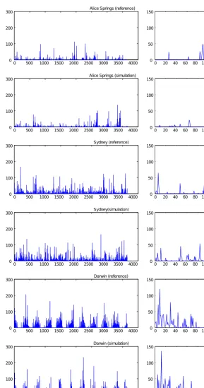
Fig. 2. Visual comparison between the simulated and the reference daily rainfall [mm] time-series: 10-years

(left column) and 100-days (right column) random samples. 21

Figure 2. Visual comparison between the simulated and the reference daily rainfall (mm) time series: 10-year (left-column panels) and

100-day (right-column panels) random samples.

4.1 Visual comparison

Figure 2 shows the comparison between random samples from both the simulated and the reference time series. For each data set, the generated rainfall looks similar to the

Fig. 3. qq-plots of the empirical probability rainfall amount [mm] distributions: median of the realizations

(blue dots), 5th and 95th percentile (dashed lines). The bisector (solid line) indicates the exact quantile match.

22

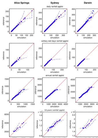
Figure 3. qq plots of the empirical probability rainfall amount (mm) distributions: median of the realizations (blue dots), 5th and 95th

per-centiles (dashed lines). The bisector (solid line) indicates the exact quantile match.

rainfall events, visible in the 100-day samples. These aspects are evaluated quantitatively in the following sections. 4.2 Multiple-scale probability distribution

The qq plots of the rainfall empirical distributions are pre-sented in Fig. 3, where all the range of quantiles is consid-ered. The distribution of the daily rainfall (computed on wet days only) is generally respected, although some extremes that are present only once in the reference and, in particular, at the start or end of the time series, may not appear in the

Fig. 4. Box-plots of the average wet days probability, mean daily rainfall amount [mm] and its standard

deviation per month. The solid line indicates the reference.

Fig. 5. Box-plots of the average extremes per month [mm]. The solid line indicates the reference.

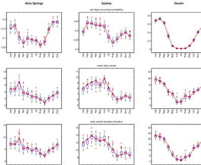
Figure 4. Box plots of the average wet-day probability, mean daily rainfall amount (mm) and its standard deviation per month. The solid line

indicates the reference.

intensities higher than the ones found in the TI at the scale of the simulated signal.

On the contrary, the distribution of the rainfall amount on the solitary wet days is accurately respected, with some real-izations including higher extremes than the reference. More importantly, the annual and 10-year rainfall distributions are correctly reproduced and do not show overdispersion. This phenomenon, common among the classical techniques based on daily scale conditioning, consists in the scarce represen-tation of the extremes and underestimation of the variance at the higher scale. This problem is avoided here because a variable dependence is considered, up to a 5000-day radius on the 365 MA auxiliary variable, that helps preserving the low-frequency fluctuations. We also see that, at this scale, DS is capable of generating extremes higher than those found in the reference, meaning that new patterns have been gener-ated using the same values at the daily scale. This results is purely based on the reproduction of higher-scale patterns: the acceptance threshold value chosen for the 365 MA auxiliary variable allows enough freedom to generate new patterns al-though maintaining an unbiased distribution. Nevertheless, this approach is not meant to replace a specific technique to predict long recurrence-time events at any temporal scale,

since it is not focused on modeling the tail of the probability distribution.

4.3 Annual seasonality and extremes

Figure 4 shows the principal indicators describing the annual seasonality of the reference and the generated time series: each different season is accurately reproduced by the algo-rithm, with almost no bias. The probability of having a wet day, usually imposed by a prior model in the classical para-metric techniques, is indirectly obtained by sampling from the rainfall patterns of the appropriate period of the year. This goal is mainly achieved using the auxiliary variables tr1 and tr2 as conditioning data (see Sect. 3).

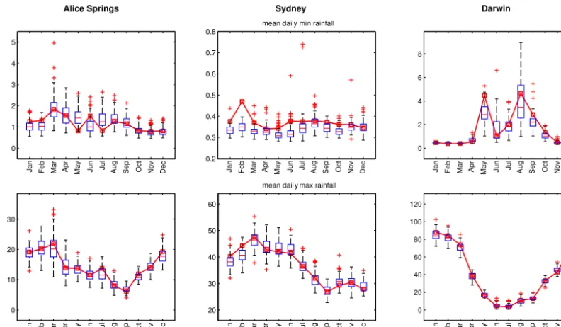
The simulation of the average extremes, shown in Fig. 5, also follows the reference rather accurately.

4.4 Rainfall patterns and verbatim copy

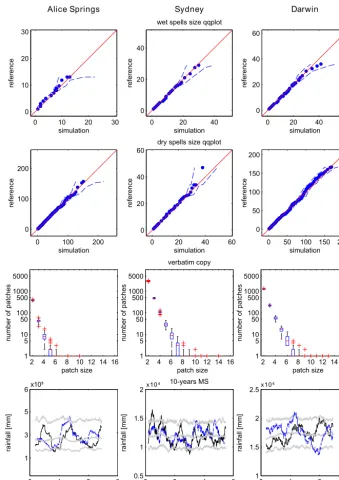
The statistical indicators regarding the dry/wet patterns shown in Fig. 6 demonstrate the efficiency of the proposed DS setup in simulating long droughts or wet periods ac-cording to the training data set: the dry- and wet-spell

F. Oriani et al.: Simulation of rainfall time series from different climatic regions 3025

deviation per month. The solid line indicates the reference.

Fig. 5. Box-plots of the average extremes per month [mm]. The solid line indicates the reference.

23

Figure 5. Box plots of the average extremes per month (mm). The solid line indicates the reference.

distributions are preserved and extremes higher than the ones present in the TI are also simulated.

The verbatim-copy box plots show the distribution of the time series pieces exactly copied from the TI as a function of their size for the ensemble of the realizations: the num-ber of patches decreases exponentially with their size. The phenomenon is mainly limited to a maximum of a few 8-day patches, with isolated cases of up to 14 days.

The 10-year rainfall moving sum, shown at the bottom of Fig. 6, illustrates the low-frequency time series structure: the quantiles of the simulations at each time step confirm that the overall variability is correctly simulated, but the local fluc-tuations do not match the reference. For example, the Dar-win reference series shows a clear upward trend which is not present in the superposed randomly picked DS realization. Generally, the TI is supposed to be stationary or the nonsta-tionarity should be at least described by an auxiliary variable. If it is not the case, as for the Darwin time series, the algo-rithm honors the marginal distribution of the reference, but it does not reproduce a specific trend. This problem is treated separately in Sect. 4.6.

The minimum moving average on different window lengths of up to 60 years (Fig. 7) gives information about the long-term structure of rainfall. The zero values are in ac-cordance with the dry spell distribution shown in Fig. 6; for example, Alice Springs presents a zero-minimum moving av-erage until 5 months, meaning that it contains dry spells of this length. Alice Springs and Sydney show a very different long-term structure: the former with long dry spells, the lat-ter with a wider range of minimum values. Darwin presents

the peculiarities of both climates with a sharp rising from the annual to the 60-year scale.

According to this indicator, the simulation of the long-term structure is fairly accurate. The negative bias, lower than 0.5 mm, shows a modest tendency to underestimate the min-imum moving average from the annual to the decennial scale for wet climates such as Sydney and Darwin.

4.5 Linear time-dependence

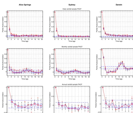
The specific linear time-dependence of the generated and ref-erence signals has been evaluated at different scales using the sample PACF (Fig. 8, Eq. 4).

At the daily scale, the data show the same level of auto-correlation at lag 1 and a low but significant linear depen-dence until lag 3 for Alice Springs and Sydney, while Darwin presents a longer tailing which asymptotically approaches the confidence bounds of an uncorrelated noise. The DS sim-ulation shows a tendency to a slight underestimation of the lag 1 PACF, with a maximum error around 0.1 for Sydney. Since the algorithm operates in a nonparametric way and im-poses a variable time-dependence, the eventuality of modi-fying the structure of the daily signal cannot be excluded a priori, for this reason the PACF has been calculated up to the 20th lag, assuring that no extra linear-dependence has been introduced.

Fig. 6. Main indicators describing the rainfall pattern: qq-plots of the dry and wet spells [days] distributions,

verbatim copy box-plots as function of the patch size [days] and daily 10-years Moving Sum (M S) time-series

[mm] of the reference (black line), median, 5-th and 95-th percentile of the realizations (gray lines) and a

randomly picked simulation (dashed blue line).

24

Figure 6. Main indicators describing the rainfall pattern: qq plots of the dry- and wet-spell (days) distributions, verbatim-copy box plots as

function of the patch size (days) and daily 10-year MS time series (mm) of the reference (black line), median, 5th and 95th percentiles of the realizations (gray lines) and a randomly picked simulation (dashed blue line).

reflected in the PACF. The simulation follows the reference fairly well, with a maximum error of approximately±0.1.

At the annual scale, the limited length of the time series leads to wider confidence bounds for the nonsignificant val-ues (see Sect. 3.2). The reference does not show a clear lin-ear time-dependence structure which is not similarly repro-duced by the simulation. Some more relevant discrepancies are present in the Darwin series, showing a more discontin-uous structure. However, using such a limited data set for

the timescale considered here, it is difficult to determine if the reference PACF is really indicative of an effective linear dependence.

4.6 Nonstationary simulation

F. Oriani et al.: Simulation of rainfall time series from different climatic regions 3027

0 0.1 0.2 0.3 0.4 0.5 0.6 0.7 0.8 0.9

20d 2m 5m 13m 3y 8y 22y 60y

minimum moving average

0 0.5 1 1.5 2 2.5 3 3.5

20d 2m 5m 13m 3y 8y 22y 60y

0 0.5 1 1.5 2 2.5 3 3.5 4 4.5 5

20d 2m 5m 13m 3y 8y 22y 60y

Fig. 7. Minimum moving average of daily rainfall [mm] for different running window lengths (days, months

or years). The solid line indicates the reference.

Fig. 8. Sample Partial Autocorrelation Function (PACF) of the daily, monthly and annual rainfall signal: the

reference (solid line), 100 DS simulations (box-plots), and confidence bounds for the negligible autocorrelation

indexes (dashed lines).

Figure 7. Minimum moving average of daily rainfall (mm) for different running window lengths (days, months or years). The solid line

indicates the reference.

0 0.1 0.2 0.3 0.4 0.5 0.6 0.7 0.8 0.9

20d 2m 5m 13m 3y 8y 22y 60y 0 0.5 1 1.5 2 2.5 3

20d 2m 5m 13m 3y 8y 22y 60y

0 0.5 1 1.5 2 2.5 3 3.5 4 4.5 5

20d 2m 5m 13m 3y 8y 22y 60y

Fig. 7. Minimum moving average of daily rainfall [

mm

] for different running window lengths (days, months

or years). The solid line indicates the reference.

Fig. 8. Sample Partial Autocorrelation Function (PACF) of the daily, monthly and annual rainfall signal: the

reference (solid line), 100 DS simulations (box-plots), and confidence bounds for the negligible autocorrelation

indexes (dashed lines).

Figure 8. Sample PACF of the daily, monthly and annual rainfall signal. Reference (solid line), 100 DS simulations (box plots), and

confi-dence bounds for the negligible autocorrelation indexes (dashed lines).

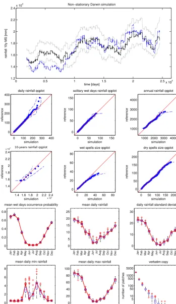
Fig. 9. Darwin daily rainfall non-stationary simulation: 10-years Moving Sum time-series (top) of the reference

(black line), median, 5-th and 95-th percentile of the realizations (gray lines) and a randomly picked simulation

26

Figure 9. Darwin daily rainfall nonstationary simulation: 10-year moving sum time series (top panel) of the reference (black line), median,

sum plot shows that the trend and low-frequency fluctuation present in the reference are accurately simulated: the median of the realizations follows the reference and a variability of about 4 m between the 5th and 95th percentiles is present. Regarding the other considered statistical indicators, the per-formance appears to be essentially the same as for the sta-tionary simulation: the only remarkable difference is a mod-est positive bias in the maximum wet-period length.

The fact that, to impose the trend, the sampling is restricted to a local region of the reference reduces the local variabil-ity with respect to the stationary simulation. Consequently, a modest increase of the verbatim-copy effect occurs.

This technique can be applied in cases where a specific nonstationarity extended to high-order moments should be imposed; e.g., exploring the uncertainty of a given past or future scenario, where a simple trend or seasonality adjust-ment is insufficient and an overly complex parametric model would be necessary to preserve the same long-term behavior.

5 Conclusions

The aim of the paper is to present an alternative daily rainfall simulation technique based on the direct sampling algorithm, belonging to the multiple-point statistics family. The main principle of the technique is to resample a given data set us-ing a pattern-similarity rule. Usus-ing a random simulation path and a nonfixed pattern dimension, the technique allows im-posing a variable time-dependence and reproducing the refer-ence statistics at multiple scales. The proposed setup, suitable for any type of rainfall, includes the simulation of the daily rainfall time series together with a series of auxiliary vari-ables including a categorical variable describing the dry/wet pattern, the 2-day moving sum which helps in respecting the lag 1 autocorrelation, the 365-day moving average to con-dition upon interannual fluctuations and two coupled theo-retical periodic functions describing the annual seasonality. Since all the variables are automatically computed from the rainfall data, no additional information is needed.

The technique has been tested on three different climates of Australia: Alice Springs (desert), Sydney (temperate) and Darwin (tropical savannah). Without changing the simula-tion parameters, the algorithm correctly simulates both the rainfall occurrence structure and amount distribution up to the decennial scale for all the three climates, avoiding the problem of overdispersion, which often affects daily rainfall simulation techniques. Being based on resampling, the algo-rithm can only generate data which are present in the train-ing data set, but they can be aggregated differently, simulat-ing new extremes in the higher-scale rainfall and dry-/wet-pattern distributions. The technique is not meant to be used as a tool to explore the uncertainty related to long recurrence-time events, but rather to generate extremely realistic repli-cates of the datum, to be used as inputs in hydrologic models.

Reproducing the specific trend found in the data is also possible by making use of an additional auxiliary variable which simply restricts the sampling to a local portion of the TI. In this way, any type of nonstationarity present in the TI is automatically imposed on the simulation. The Darwin exam-ple demonstrates the efficiency of this approach in reproduc-ing 100 different realizations showreproduc-ing the same type of trend and marginal distribution. This setup can be useful to simu-late multiple realizations of a specific nonstationary scenario regardless of its complexity.

In conclusion, the direct sampling technique used with the proposed generic setup can produce realistic daily rain-fall time-series replicates from different climates without the need of calibration or additional information. The generality and the total automation of the technique makes it a powerful tool for routine use in scientific and engineering applications.

Acknowledgements. This research was funded by the Swiss

National Science Foundation (project no. 134614) and supported by the National Centre for Groundwater Research and Training (University of New South Wales). The data set used in this paper is courtesy of the Australian Bureau of Meteorology (BOM). Edited by: E. Morin

References

Allard, D., Froidevaux, R., and Biver, P.: Conditional simulation of multi-type non stationary markov object models respecting spec-ified proportions, Math. Geol., 38, 959–986, 2006.

Arpat, G. and Caers, J.: Conditional simulation with patterns, Math. Geol., 39, 177–203, 2007.

Bardossy, A. and Plate, E. J.: Space-time model for daily rainfall using atmospheric circulation patterns, Water Resour. Res., 28, 1247–1259, doi:10.1029/91WR02589, 1992.

Box, G. E. and Jenkins, G. M.: Time series analysis, forecasting and control, Holden-Day, Oakland, CA, 1976.

Briggs, W. M. and Wilks, D. S.: Estimating monthly and seasonal distributions of temperature and precipitation using the new CPC long-range forecasts, J. Climate, 9, 818–826, doi:10.1175/1520-0442(1996)009<0818:EMASDO>2.0.CO;2, 1996.

Buishand, T. A. and Brandsma, T.: Multisite simulation of daily precipitation and temperature in the Rhine basin by nearest-neighbor resampling, Water Resour. Res., 37, 2761–2776, doi:10.1029/2001WR000291, 2001.

Chugunova, T. L. and Hu, L. Y.: Multiple-point simulations con-strained by continuous auxiliary data, Math. Geosci., 40, 133– 146, doi:10.1007/s11004-007-9142-4, 2008.

Clark, M. P., Gangopadhyay, S., Brandon, D., Werner, K., Hay, L., Rajagopalan, B., and Yates, D.: A resampling procedure for gen-erating conditioned daily weather sequences, Water Resour. Res., 40, W04304, doi:10.1029/2003WR002747, 2004.

Coe, R. and Stern, R. D.: Fitting models to daily rainfall data, J. Appl. Meteorol., 21, 1024–1031, doi:10.1175/1520-0450(1982)021<1024:FMTDRD>2.0.CO;2, 1982.

Guardiano, F. and Srivastava, R.: Multivariate geostatistics: beyond bivariate moments, Geostatistics-Troia, 1, 133–144, 1993. Harrold, T. I., Sharma, A., and Sheather, S. J.: A nonparametric

model for stochastic generation of daily rainfall occurrence, Wa-ter Resour. Res., 39, 1300, doi:10.1029/2003WR002182, 2003a. Harrold, T. I., Sharma, A., and Sheather, S. J.: A nonparametric model for stochastic generation of daily rainfall amounts, Water Resour. Res., 39, 1343, doi:10.1029/2003WR002570, 2003b. Hay, L. E., Mccabe, G. J., Wolock, D. M., and Ayers, M. A.:

Sim-ulation of precipitation by weather type analysis, Water Resour. Res., 27, 493–501, doi:10.1029/90WR02650, 1991.

Honarkhah, M. and Caers, J.: Stochastic simulation of patterns us-ing distance-based pattern modelus-ing, Math. Geosci., 42, 487– 517, 2010.

Hu, L. Y., Liu, Y., Scheepens, C., Shultz, A. W., and Thomp-son, R. D.: Multiple-Point Simulation with an Existing Reser-voir Model as Training Image, Math. Geosci., 46, 227–240, doi:10.1007/s11004-013-9488-8, 2014.

Hughes, J. and Guttorp, P.: A class of stochastic models for relating synoptic atmospheric patterns to regional hydrologic phenom-ena, Water Resour. Res., 30, 1535–1546, 1994.

Hughes, J., Guttorp, P., and Charles, S.: A non-homogeneous hid-den Markov model for precipitation occurrence, J. Roy. Stat. Soc. Ser. C, 48, 15–30, 1999.

Jones, P. G. and Thornton, P. K.: Spatial and temporal variability of rainfall related to a third-order Markov model, Agr. Forest Mete-orol., 86, 127–138, doi:10.1016/S0168-1923(96)02399-4, 1997. Kaplan, E. and Meier, P.: Non-parametric estimation from in-complete observations, J. Am. Stat. Assoc., 53, 457–481, doi:10.2307/2281868, 1958.

Katz, R. W. and Parlange, M. B.: Effects of an index of atmospheric circulation on stochastic properties of precipitation, Water Re-sour. Res., 29, 2335–2344, doi:10.1029/93WR00569, 1993. Katz, R. W. and Zheng, X. G.: Mixture model for overdispersion

of precipitation, J. Climate, 12, 2528–2537, doi:10.1175/1520-0442(1999)012<2528:MMFOOP>2.0.CO;2, 1999.

Kiely, G., Albertson, J. D., Parlange, M. B., and Katz, R. W.: Conditioning stochastic properties of daily precipitation on in-dices of atmospheric circulation, Meteorol. Appl., 5, 75–87, doi:10.1017/S1350482798000656, 1998.

Lall, U. and Sharma, A.: A nearest neighbor bootstrap for resam-pling hydrologic time series, Water Resour. Res., 32, 679–693, doi:10.1029/95WR02966, 1996.

Lall, U., Rajagopalan, B., and Tarboton, D. G.: A nonparametric wet/dry spell model for resampling daily precipitation, Water Resources Research, 32, 2803–2823, doi:10.1029/96WR00565, 1996.

Mariethoz, G. and Renard, P.: Reconstruction of Incomplete Data Sets or Images Using Direct Sampling, Math. Geosci., 42, 245– 268, doi:10.1007/s11004-010-9270-0, 2010.

Mariethoz, G., Renard, P., and Straubhaar, J.: The direct sampling method to perform multiple-point geostatistical simulations, Wa-ter Resour. Res., 46, W11536, doi:10.1029/2008WR007621, 2010.

Meerschman, E., Pirot, G., Mariethoz, G., Straubhaar, J., Van Meirvenne, M., and Renard, P.: A practical guide to per-forming multiple-point statistical simulations with the Di-rect Sampling algorithm, Comput. Geosci., 52, 307–324, doi:10.1016/j.cageo.2012.09.019, 2013.

Mehrotra, R. and Sharma, A.: A semi-parametric model for stochastic generation of multi-site daily rainfall exhibit-ing low-frequency variability, J. Hydrol., 335, 180–193, doi:10.1016/j.jhydrol.2006.11.011, 2007a.

Mehrotra, R. and Sharma, A.: Preserving low-frequency variability in generated daily rainfall sequences, J. Hydrol., 345, 102–120, doi:10.1016/j.jhydrol.2007.08.003, 2007b.

Ndiritu, J.: A variable-length block bootstrap method for multi-site synthetic streamflow generation, Hydrolog. Sci. J., 56, 362–379, doi:10.1080/02626667.2011.562471, 2011.

Rajagopalan, B. and Lall, U.: A k-nearest-neighhor simulator for daily precipitation and other weather variables, Water Resour. Res., 35, 3089–3101, doi:10.1029/1999WR900028, 1999. Sharma, A. and Mehrotra, R.: Rainfall generation, in: Rainfall: state

of the science, no. 191 in Geophysical Monograph Series, AGU, Washington, D.C., 215–246, 2010.

Srikanthan, R.: Stochastic generation of daily rainfall data using a nested model, 57th Canadian Water Resources Association Annual Congress, 16–18 June 2004, Montreal, Canada, 16–18, 2004.

Srikanthan, R.: Stochastic generation of daily rainfall data using a nested transition probability matrix model, in: 29th Hydrology and Water Resources Symposium: Water Capital, 20–23 Febru-ary 2005, Rydges Lakeside, Canberra, p. 26, 2005.

Srikanthan, R. and Pegram, G. G. S.: A nested multisite daily rainfall stochastic generation model, J. Hydrol., 371, 142–153, doi:10.1016/j.jhydrol.2009.03.025, 2009.

Srinivas, V. V. and Srinivasan, K.: Hybrid moving block bootstrap for stochastic simulation of multi-site multi-season streamflows, J. Hydrol., 302, 307–330, doi:10.1016/j.jhydrol.2004.07.011, 2005.

Straubhaar, J.: MPDS technical reference guide, Centre d’hydrogeologie et geothermie, University of Neuchâtel, Neuchâtel, 2011.

Straubhaar, J., Renard, P., Mariethoz, G., Froidevaux, R., and Besson, O.: An improved parallel multiple-point algorithm us-ing a list approach, Math. Geosci., 43, 305–328, 2011.

Strebelle, S.: Conditional simulation of complex geological struc-tures using multiple-point statistics, Math. Geol., 34, 1–21, 2002. Tahmasebi, P., Hezarkhani, A., and Sahimi, M.: Multiple-point geostatistical modeling based on the cross-correlation functions, Comput. Geosci., 16, 779–797, 2012.

Vogel, R. M. and Shallcross, A. L.: The moving blocks bootstrap versus parametric time series models, Water Resour. Res., 32, 1875–1882, doi:10.1029/96WR00928, 1996.

Wallis, T. W. R. and Griffiths, J. F.: Simulated meteorological in-put for agricultural models, Agr. Forest Meteorol., 88, 241–258, doi:10.1016/S0168-1923(97)00035-X, 1997.

Wang, Q. J. and Nathan, R. J.: A daily and monthly mixed algorithm for stochastic generation of rainfall time series, 27th Hydrology and Water Resources Symposium: Water Challenge – Balancing the Risks, 20–23 May 2002, Melbourne, Australia, p. 698, 2002. Wilby, R. L.: Modelling low-frequency rainfall events using airflow indices, weather patterns and frontal frequencies, J. Hydrol., 212, 380–392, doi:10.1016/S0022-1694(98)00218-2, 1998.

Wojcik, R. and Buishand, T. A.: Simulation of 6-hourly rainfall and temperature by two resampling schemes, J. Hydrol., 273, 69–80, doi:10.1016/S0022-1694(02)00355-4, 2003.

Wojcik, R., McLaughlin, D., Konings, A., and Entekhabi, D.: Con-ditioning stochastic rainfall replicates on remote sensing data, IEEE T. Geosci. Remote, 47, 2436–2449, 2009.

Woolhiser, D. A., Keefer, T. O., and Redmond, K. T.: South-ern oscillation effects on daily precipitation in the south-western United-States, Water Resour. Res., 29, 1287–1295, doi:10.1029/92WR02536, 1993.

Young, K. C.: A multivariate chain model for simulating climatic parameters from daily data, J. Appl. Meteorol., 33, 661–671, doi:10.1175/1520-0450(1994)033<0661:AMCMFS>2.0.CO;2, 1994.