A conceptual, distributed snow redistribution model

www.hydrol-earth-syst-sci.net/19/4517/2015/ doi:10.5194/hess-19-4517-2015

© Author(s) 2015. CC Attribution 3.0 License.

A conceptual, distributed snow redistribution model

S. Frey and H. Holzmann

Institute of Water Management, Hydrology and Hydraulic Engineering, University of Natural Resources and Life Sciences, Vienna, Austria

Correspondence to: S. Frey ([email protected])

Received: 10 December 2014 – Published in Hydrol. Earth Syst. Sci. Discuss.: 14 January 2015 Revised: 26 October 2015 – Accepted: 4 November 2015 – Published: 12 November 2015

Abstract. When applying conceptual hydrological models using a temperature index approach for snowmelt to high alpine areas often accumulation of snow during several years can be observed. Some of the reasons why these “snow tow-ers” do not exist in nature are vertical and lateral transport processes. While snow transport models have been devel-oped using grid cell sizes of tens to hundreds of square me-tres and have been applied in several catchments, no model exists using coarser cell sizes of 1 km2, which is a common resolution for meso- and large-scale hydrologic modelling (hundreds to thousands of square kilometres). In this paper we present an approach that uses only gravity and snow den-sity as a proxy for the age of the snow cover and land-use information to redistribute snow in alpine basins. The results are based on the hydrological modelling of the Austrian Inn Basin in Tyrol, Austria, more specifically the Ötztaler Ache catchment, but the findings hold for other tributaries of the river Inn. This transport model is implemented in the dis-tributed rainfall–runoff model COSERO (Continuous Semi-distributed Runoff). The results of both model concepts with and without consideration of lateral snow redistribution are compared against observed discharge and snow-covered ar-eas derived from MODIS satellite images. By means of the snow redistribution concept, snow accumulation over several years can be prevented and the snow depletion curve com-pared with MODIS (Moderate Resolution Imaging Spectro-radiometer) data could be improved, too. In a 7-year period the standard model would lead to snow accumulation of ap-proximately 2900 mm SWE (snow water equivalent) in high elevated regions whereas the updated version of the model does not show accumulation and does also predict discharge with more accuracy leading to a Kling–Gupta efficiency of 0.93 instead of 0.9. A further improvement can be shown in the comparison of MODIS snow cover data and the

cal-culated depletion curve, where the redistribution model in-creased the efficiency (R2) from 0.70 to 0.78 (calibration) and from 0.66 to 0.74 (validation).

1 Introduction

The reasons for that are either wind or gravitationally in-duced lateral snow distribution processes (Elder et al., 1991; Winstral et al., 2002). Resulting snow depths are not uni-formly distributed in space but vary within large ranges (Hel-fricht et al., 2014). When changing the focus from micro (e.g. several square metres) to meso-scales (e.g. one to sev-eral square kilometres), variations become less (Melvold and Skaugen, 2013). The intention of the applied snow redistribu-tion concept was (i) to prevent the artefacts of “snow towers” and (ii) to develop a concept which considers gravity driven lateral snow transport with reasonable and plausible process depiction.

1.1 Theoretical background of snow cover variations During the accumulation period, according to Liston (2004), primarily three mechanisms are responsible for these vari-ations: (i) snow–canopy interactions in forest covered re-gions, (ii) wind-induced snow redistribution and (iii) oro-graphic influences on snow fall. These mechanisms influence snow cover patterns on scales ranging from the micro to the macro scale. Spatial snow cover variability beneath canopies is mainly affected by different tree species (deciduous vs. coniferous trees) influencing leaf area index, height and den-sity of the canopy and gap sizes (Garvelmann et al., 2013; Liston, 2004; Pomeroy et al., 2002).

Besides the impact of vegetation, wind is the most domi-nant factor influencing snow patterns in alpine terrain. Snow is transported from exposed ridges to the lee side of these ridges, valleys and vegetation-covered areas (Essery et al., 1999; Liston and Sturm, 1998; Rutter et al., 2009; Winstral et al., 2002). One has to be aware that besides of the physical transport of solid snow wind also stimulates sublimation pro-cesses (Liston and Sturm, 1998; Strasser et al., 2008). Wind influences snow depth distributions on the scale of hundreds to 1000 m2(Dadic et al., 2010a).

The third mechanism (orographic effect) influences snow patterns on a larger scale of one to several kilometres (e.g. Barros and Lettenmaier, 1994). Non-uniform snow dis-tributions are caused by interactions of the atmosphere (air pressure, humidity, atmospheric stability) with topography (Liston, 2004).

In addition to these processes, avalanches play a role in snow redistribution (Lehning and Fierz, 2008; Lehning et al., 2002; Sovilla et al., 2010). In steep terrain, avalanches de-pend mainly on the slope angle and are capable of transport-ing large snow masses over distances of tens to hundreds of metres (Dadic et al., 2010b; Sovilla et al., 2010).

During the ablation period, spatial snow distributions are mainly influenced by differences in snowmelt behaviour. On the Northern Hemisphere, on south-facing slopes, rates of snowmelt are generally enhanced compared to north-facing slopes due to the inclination of radiation. Also vegetation in-fluences melting behaviour. Shading reduces snowmelt com-pared to direct sunlight. Enhanced emitted long wave

radia-tion due to warm bare rocks or trees increases the melt rate (Garvelmann et al., 2013; Pohl et al., 2014).

1.2 Modelling approaches

There exist a plenty of model concepts to simulate the snow redistribution in mountainous areas, ranging from simple conceptual models to complex, physically based ones. The latter attempt to consider all energy fluxes and therefore show a huge data demand with respect to meteorological input. Usually this type requires high spatial resolution of the model domain. Alternatively, the conceptual models can also be easily applied for meso- and macro-scale basins, where the spatial resolution generally shows coarser grid spacing. This is the case for the introduced study where the entire basin of the river Inn was modelled (see Frey et al., 2014), and selec-tive results of the Ötztal are presented.

Generally, there are several ways of coping with inten-sive snow accumulations in hydrological models, in partic-ular (i) adapting the meteorological input data, (ii) the ap-plication of physically based models to solve the full en-ergy balance and considering the wind-induced snow drift and (iii) conceptual models using topographic information for lateral snow transport. In the following some descriptions and references of the respective concepts are given.

A common approach is editing the meteorological input (Dettinger et al., 2004). For instance, many models use a constant yet adjustable lapse rate for interpolating temper-ature with elevation (Holzmann et al., 2010; Koboltschnig et al., 2008). Besides temperature, precipitation gradients are often adjusted to fit observed and modelled target variables (e.g. snow patterns or runoff) (Huss et al., 2009b; Schöber et al., 2014). Justification for doing so is the general lack of gauging stations in the summit regions (Daly et al., 1994, 2008) along with the high error of precipitation gauges (Ras-mussen et al., 2011; Williams et al., 1998). An approach presented by Jackson (1994) defining a precipitation cor-rection matrix was successfully applied in several studies (Farinotti et al., 2010; Huss et al., 2009a). Using a Doppler X-band radar capable of a spatial resolution of 75 m, Scipión et al. (2013) identified significant discrepancies between pre-cipitation patterns in 300–600 m above ground and the snow accumulation at the end of the winter period in a small area of 1.5 km2in the vicinity of Davos, Switzerland. They con-clude that snowfall variability at the height of some hundreds of metres above ground is not the driving factor of snow ac-cumulation variabilities at the scale of the radar’s resolution. Consequently, the variability of the meteorological input can-not explain the variability of snow cover patterns.

The other approach is empirical. Models following the sec-ond approach use the fact that snow patterns resemble each other every year (Helfricht et al., 2012, 2014). Since our model is following the empirical approach, too, the presented paper concentrates on that approach.

Snow accumulation gradients determined by airborne lidar measurements (Helfricht et al., 2012) were used by Schöber et al. (2014) to improve hydrological modelling using the distributed energy balance model SES (Snow and Ice Melt; Asztalos, 2004). Lidar data, however, are relatively expen-sive to obtain. A common way of dealing with snow accu-mulations without the need for intensive field campaigns is using wind speed and direction to model lateral snow trans-port (e.g. Bernhardt et al., 2009, 2010; Shulski and Seeley, 2004; Winstral et al., 2002; Liston and Sturm, 1998). Wind information may be obtained by meteorological stations or by computed wind fields. Kirchner et al. (2014) concluded from Lidar measurements in combination with meteorolog-ical stations in a catchment in California, USA, that wind measurements from only one meteorological station are of too poor quality for a useful description of wind fields for snow transport. Due to the mentioned lack of meteorologi-cal stations in high elevations, the use of computer-generated wind fields seems appealing. This information has been suc-cessfully used to model snow redistributions in small scales of 30 m (Bernhardt et al., 2009, 2010, 2012). Those models using wind information have in common that they are com-putationally intensive as they require data in high spatial res-olution (e.g. from 100 to thousands of square metres). Wind fields may also be generated by regional circulation mod-els (RCMs). However, these wind fields have shown to be er-roneous (Nikulin et al., 2011) and therefore are not useful for direct implementation in redistribution models. A combined approach using gravity and wind-induced snow transport was presented by Schöber et al. (2014), who used a distributed energy balance model with a resolution of 50×50 m. The SnowSlide model (Bernhardt and Schulz, 2010) applied to the Watzmann massif, Germany, only accounts for gravita-tionally induced snow transport.

The mentioned model approaches have in common that they operate on spatial scales of tens to hundreds of me-tres. However, due to some available databases for vegeta-tion and meteorology (Haiden et al., 2011; Hiebl and Frei, 2015; Masson et al., 2003; Oubeidillah et al., 2014), many models operate on cell sizes of 1 km2or more (e.g. Ander-sen et al., 2001; HenrikAnder-sen et al., 2003; Mauser and Bach, 2009; Safeeq et al., 2014). While the main driving physical processes on the scale of these data sets might differ from the scale of the modelling approaches described above, the difficulties of snow accumulations also occur when models with grid cell sizes of 1×1 km are applied to mountainous regions. Yet, to our knowledge, no model for redistributing snow on a 1×1 km grid size exists. In this paper we present a simple approach to deal with snow in high mountainous re-gions and its application in the catchment of Ötztaler Ache

in Tyrol, Austria. Since the model uses meteorological input from INCA (Integrated Nowcasting through Comprehensive Analysis; Haiden et al., 2011) that already account for meteo-rological corrections, we focus on snow redistribution rather than editing the input data. As already mentioned, the two main objectives in this respect are to achieve a better model efficiency regarding runoff and to avoid the existence of snow towers at high altitudes.

2 Model description

2.1 Hydrological model COSERO

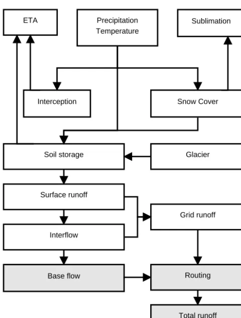
COSERO (Continuous Semi-distributed Runoff) is a spa-tially distributed conceptual hydrological model which is similar to the HBV model (Bergström, 1976). In the pre-sented paper it uses 1×1 km grid cells. Originally devel-oped for modelling discharge of the Austrian rivers Enns and Steyr (Nachtnebel et al., 1993), it has recently been used for different purposes like climate change studies (e.g. Kling et al., 2012, 2014b; Stanzel and Nachtnebel, 2010), investi-gating the role of evapotranspiration in high alpine regions (Herrnegger et al., 2012) and operational runoff forecasting (Stanzel et al., 2008). Potential evapotranspiration is calcu-lated using the Thornthwaite method (Thornthwaite, 1948). Discharge due to rainfall and snow-/ice melt is estimated us-ing the same non-linear function of soil moisture as the orig-inal HBV. In this study, the model is run using daily time steps. It is, however, capable of using hourly or monthly time steps. In the latter case, intra-monthly variations are consid-ered for snow and interception processes as well as for soil moisture (Kling et al., 2014b). A schematic overview of the model is given in Fig. 1 and a detailed description of the model can be found in Kling et al. (2014a), where the model was applied to several catchments across Europe, Africa and Australia. However, in Kling et al. (2014a) snow parame-ters were not calibrated and therefore the snow module is not fully explained in detail in their paper. This will be done in the following. Equations (1)–(7) and Eq. (10) were taken from the original model by Stanzel and Nachtnebel (2010), all other methods were developed in the present study.

ETA Precipitation Temperature

Sublimation

Interception Snow Cover

Soil storage

Surface runoff

Interflow

Base flow

Grid runoff

Routing

Total runoff Glacier

Figure 1. Flow chart of the conceptual model COSERO. White parts represent distributed processes, greyish parts are calculated on a subbasin scale. Snow transport is implemented in the snow cover module.

shelter, vegetation and elevation (Hiemstra et al., 2006). The properties of each class are treated unique as Eqs. (1)–(13) apply to every snow class separately. Consequently the log-normal distribution within a grid cell may be disturbed by the processes of melting, sublimation, refreezing and redis-tribution to other grid cells. Once fallen, snow redisredis-tribution between the snow classes within a single grid cell is not con-sidered. A scheme of the composition of a snow class is il-lustrated in Fig. 2a. The snow water equivalent (SSWEt) of a

given dayt per class is calculated by Eq. (1) wherePRt and PSt are liquid and solid precipitation in millimetres,

respec-tively, Mt is snowmelt andESt is sublimation of snow. All

variables are given in millimetres of SWE.

SSWEt =SSWEt−1+PRt +PSt−Mt−ESt (1)

Snowmelt is calculated by a temperature index approach (see for example Hock, 2003). Equation (2) is used:

Mt=min SSWEt;PRt ·ε·TAIRt +Dft·TAIRt

, (2)

whereMt is snowmelt (mm),εis the ratio of specific heat of water and melting energy, TAIRt is the (mean) daily air

Liquid water content [mm SWE] Dry snow bound by

vegetation

[mm SWE] Snow depth (S) [mm] Dry snow available for

redistribution [mm SWE]

Hv

[mm]

b) a)

[mm SWE]

Snow classes

Figure 2. Schematic view of the snow cover in COSERO. (a) Com-position of one snow class. Vegetation or surface roughness defines the threshold value (Hv) to hold back an amount of snow. (b) View of one grid cell including five snow classes each of which is com-posed in the way shown in (a). Snowfall is distributed log-normally throughout the classes (dashed lines in b). Note that snow depthSis given in millimetres while all other parameters regarding snow are given in millimetres of SWE.

temperature (◦_{C) andD}

ft (mm

◦_C−1_{) is the snowmelt factor}

of a given daytestimated by Eq. (3):

Dft =

−cos

J· 2π

365

·DU−DL

2 +

DU−DL

2

·MREDt (3)

with

MREDt =

( _D

RED, Sfresh≥SCRIT

MREDt−1+

1−MREDt−1

5 , Sfresh< SCRIT

, (4)

whereJ is the Julian day of the year (–),DUandDLare the

upper and lower boundaries ofDf(mm◦C−1), respectively,

andMRED(–) is a reduction factor to account for the higher

albedo caused by freshly fallen snow calculated by Eq. (4).

SCRIT(mm) is the critical snow depth of fresh snow

neces-sary to increase the albedo, whereasSfreshis the actual depth

of fresh snow (mm) fallen within one time step. For fresh snow depth larger thanSCRIT,MREDis set to a reduced

melt-ing factorDRED(–).

Whether precipitation occurs in form of snow or rain is controlled by two parametersTPSandTPR, defining the

tem-perature range where snow and rain occur simultaneously. At and above temperatureTRPprecipitation is pure liquid, at and

belowTPSprecipitation is pure solid. In between those two

boundaries, the proportion of solid to liquid precipitation is estimated linearly.

(mm) is the potential evapotranspiration andERis a

correc-tion factor to reduceEP. Sublimation is considered only for

snow classes actually covered by snow. Hence, if a grid cell is partly snow free (this can be the case if one subgrid class has no snow cover due to melting), sublimation is estimated for the snow-covered part only. For the uncovered classes, evapotranspiration according to the Thornthwaite method is applied.

ESPt =EPt·ER (5)

The snow cover in COSERO is treated as porous medium and therefore is able to store a certain amount of liquid wa-ter (Sl, m3kg−1) in dependency of the snowpack density (ρ)

calculated using Eq. (6).

Slt = SSWEt−Slt−1

· SlMAX−(ρ−ρMAX)·Slρ

(6)

whereSlMAX(m3kg−1) is the maximum water holding

ca-pacity at the maximum snow density of the snowpackρMAX

(kg m−3) andSlρ(–) describes the decrease of water holding capacity with increasing snow densityρ.

At negative air temperatures, retained meltwater has the ability to refreeze in the snowpack. The potential amount of refrozen water (SR) is estimated by Eq. (7), whereRfis the

refreezing factor (mm◦_C−1_{). As long as there is enough}

liq-uid water in the snowpack, actual refreezing will be equal to potential refreezing.

SR=

0, TAIRt >0

Rf· TAIRt·(−1)

, TAIRt ≤0

(7)

Refrozen water is treated in the same way as snow. The amount of water leaving the snow cover then equals snowmelt minus retained water.

Snow density (ρt) of each class is calculated using a sig-moid function shown in Eqs. (8) and (9) whereρMAX and ρMIN are the respective maximum and minimum values of ρ,TAIRis the temperature of the air mass above the snow

layer and ρscale andTscaleare scaling coefficients to

calcu-late a transition temperature (Ttr) for the estimation of the

snow density. Hereby,ρscaleadjusts the slope of the function,

whereasTscaleis responsible for a shift on thex axis. These

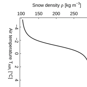
two parameters are set to fixed values of 1.2 and 1, respec-tively. The solution of Eqs. (8) and (9) is illustrated in Fig. 3 for a range of typical air temperatures, where snowfall oc-curs. Already fallen snow can reach a higher density (ρOLD)

than fresh snow. Its density is calculated using a time set-tling constant (ρSET, derived from Riley et al., 1973) until

the maximum density is reached (Eq. 10).

ρt=(ρMAX−ρMIN)·

T+t r

p

1+(Ttr)2 +1

!

·0.5+ρMIN (8)

−4

−2

0

2

4

100 150 200 250 300

Air temper

ature T

AIR

t [°C]

Snow density ρ [kg m−3]

Figure 3. Estimation of the density of snow using Eqs. (8) and (9). Minimum and maximum densities of fresh snow are 100 and 300 kg m−3, respectively.

with

Ttr= TAIRt ρscale

+Tscale, (9)

ρOLD= ρSET·

_S

SWEt ρOLD +

St 2

1+ρSET

2

. (10)

The COSERO model considers both snow and glacier ice melt processes. Ice melt (MICE) is computed by means of

a degree-day method (see Eq. 11) and uses separate parame-ter sets. Here,DICErefers to the ice melt factor (mm◦C−1).

A prerequisite of ice melt is the full depletion of the over-lying snow cover. Spatial information of glaciers are taken from the Randolph Glacier Inventory version 3.2 (Arendt et al., 2012).

MICE=DICE·TAIR (11)

2.2 Snow transport model

0.00

0.05

0.10

0.15

0.20

0.2

5

Snow density ρ [kg m−3]

Distr

ib

ution coefficient f

ρ

[−]

100 150 200 250 300 350 400 450

0° 5° 10° 15°

20° 25° 30° 35°

Figure 4. Shapes of the distribution coefficient in dependency of different slope angles and snow densities.

snowpack the higher the snow rate available for the redis-tribution routine (fρ, Eq. 13). Thus, the defined maximum density of snow (450 kg m−3) determines the threshold for snow redistribution. The availability of snow for transport is determined by a vegetation-based threshold value (Hv) for

each class of land cover. This value can also be interpreted as a roughness coefficient for areas where no or hardly any vegetation is present like in alpine and nival elevations. If the snow depth (S, mm) of a snow class of a raster cell exceeds

Hv(mm), snow transport from that cell is activated and

re-distribution is calculated by solving Eqs. (12) and (13).

SSWE(A)=max(SD−Hv;0)·fρ· 1

P

A·C (12)

with

fρ=

(ρMAX−ρD) ρMAX

·e

− ρD

ρ_MAX

· α

90, (13)

whereSSWE(A)is the amount of snow water equivalent that is redistributed from the donor cell (D) to the available acceptor cell(s) (A),ρDis the density of snow in the donor cell,ρMAX

is the possible maximum density of snow,αis the angle of the slope between the donor and acceptor cells in degree and

Cis a correction coefficient that can be calibrated.

Figure 4 illustrates the shape of the distribution coefficient

fpas a function of different elevation gradients between the

acceptor and donor cells and of the snow density. In acceptor cells redistributed snow is treated as fresh snow in the sense that it is distributed to the snow classes according to the log-normal distribution.

The model is organized in form of a loop starting at the highest grid cell (summit region) and ending at the lowest cell (outlet of the catchment). This ensures that snow can-not be redistributed into already processed grid cells. Snow will be transported downslope as long as the slope is steep enough to allow for transportation given that the density of snow is low enough (see Fig. 4). Consequently, less snow re-mains in the summit region whereas lower, rather flat grid

Elevation

a) b)

Elevation

Snow depth

Snow depth

Figure 5. Conceptual snow accumulations in mountainous regions without (a) and with (b) lateral snow transport processes. Dotted blocks represent exaggerated snow accumulations.

cells show enhanced accumulation. Although snow depths in the summits are lower, the amount of snow-covered cells stay similar as some residual snow remains in all cells due toHv

parameterization.

The concept of the redistribution model is sketched in Fig. 5. Note that although snow depths in the highest cell are prevented by the model, the number of snow-covered cells remains the same.

3 Case study in the catchment the Ötztaler Ache, Tyrol, Austria

3.1 Catchment description

The catchment of Ötztaler Ache at the Huben gauge, situated in western Austria close to the Italian border, covers an area of 511 km2and has an altitudinal range between 1185 m a.s.l. (above sea level) at the gauge at Huben and 3770 m a.s.l. at its highest peaks. Due to the use of a 1×1 km gridded DEM (digital elevation model), the highest grid cell has a mean elevation of 3450 m a.s.l., whereas the lowest cell has an ele-vation of 1250 m a.s.l. (Fig. 6). About 30 % of its area is cov-ered by vegetation, mainly pastures and meadows. Glaciers cover about 19 % leading to an annual ice melt contribution of about 25 % of the total runoff at Huben, while 41 % of the discharge has its origin in snowmelt (Weber et al., 2010). Table 1 gives an overview of the land cover.

Table 1. Land use classes used in COSERO (derived from CORINE land cover data; EEA, 1995) and their proportion in the Ötztal. Snow holding capacities Hv for each type of land use are taken from Liston and Sturm (1998) and Prasad et al. (2001).

Land use class Proportion Snow

(%) holding

capacity

Hv(mm)

Build-up areas 1.2 100

Pastures and meadows 20.9 500

Coniferous forests 8.1 2500

Sparsely vegetated areas 20.9 300

Bare rocks 29.5 200

Glaciers 19.4 200

3.2 Input data

Gridded meteorological data of precipitation and air temper-ature are required to run the model. These data are provided by the INCA data set (Haiden et al., 2011) with the same grid spacing as in the hydrological model, thus allowing a direct use in the model without the need for pre-processing. INCA data are available since 2003. The years 2003 and 2004 have been used as a warm-up period for the model. In the subsequent years no correction of meteorological data was done since INCA already accounts for elevation gradi-ents regarding air temperature and precipitation. Six land use classes were derived from the most recent CORINE data set (CLC2006 version 17, see EEA, 1995). These classes and their areal fractions in the catchment of Ötztaler Ache are given in Table 1. It should be pointed out that neither radia-tion nor wind speed or wind direcradia-tion data are necessary to run the model.

3.3 Model calibration

The hydrological model was calibrated for the period from 2005 to 2008 using Rosenbrock’s automated optimization routine (Rosenbrock, 1960). Although the model is rich in parameters, the vast majority of them have been estimated a priori according to literature (Liston and Sturm, 1998; Prasad et al., 2001) and previous work on the model (Fuchs, 2005; Kling, 2006; Nachtnebel et al., 2009). In the snow model in-cluding snow redistribution, only six parameters have been calibrated: upper and lower boundaries of snowmelt factors

DU andDL, respectively, the threshold values that control

the range where liquid and solid precipitation occur simulta-neously (TPR,TPS), the standard deviation of the log-normal

distribution of snow depth in one grid cell (NVAR) and the

calibration parameter for snow redistributionC(see Eq. 12). The limited number of optimization parameters reduces equi-finality problems. For a more detailed description of equifi-nality issues see the supplements of this article. The target

Figure 6. Elevation levels of the Ötztal using a 1×1 km grid (b). Frequency distribution of slope angles derived from 1×1 km grid is shown (a). Slopes in general are steeper in the summit regions than in the valleys. Note that instead of the average slope of a grid cell only steepest vertical gradients are plotted.

of the calibration was a good fit of runoff using the Kling– Gupta model efficiency (KGE; Gupta et al., 2009; Kling et al., 2012) as the objective function. The model was validated for the years 2009 and 2010. Both calibration and validation have been done with and without the snow transport module. In the following, model A refers to the model using snow transport, whereas model B stands for the standard model. Vegetation threshold values for snow detention were taken from previous studies (Liston and Sturm, 1998; Prasad et al., 2001). These are given in Table 1. Maximum snow density was assumed to be 450 kg m−3_{, which matches long-term}

snow measurements (Jonas et al., 2009; Schöber et al., 2014). Besides discharge in the validation period, snow cover data from MODIS (8-day maximum snow cover, version 5) satel-lite images (Hall et al., 2002) were also used to compare the performance of both models.

4 Results 4.1 Discharge

Table 2. Comparison of performances of models A and B with re-spect to snow cover and runoff. For snow cover, the coefficient of determination (R2) was used, whereas the Kling–Gupta efficiency (KGE; Gupta et al., 2009) was used for runoff.

Calibration Validation

Snow Runoff Snow Runoff

cover (KGE) cover (KGE)

(R2) (R2)

Model A 0.78 0.93 0.74 0.92

Model B 0.70 0.88 0.66 0.90

0 5 10 15 20

Runoff [mm d

−

1]

Model A (KGE = 0.9) Model B (KGE = 0.85) observed data

(model A min

us model B)

2006

−0.5 0.0 0.5 1.0 1.5 2.0 2.5

Diff

erence in Runoff [mm d

−

1]

Jan Feb Mar Apr May Jun Jul Aug Sep Oct Nov Dec Jan Differences

Figure 7. Specific runoff at the outlet at Huben is modelled with (model A) and without (model B) the snow redistribution routine.

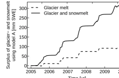
(12.1 m3s−1). This equals a relative difference of−9, up to 44 % of model A in respect to model B. In total, model A generates a surplus of about 300 mm of discharge in 5 years compared to model B (Fig. 8). About two-thirds of the ad-ditional discharge originate in enhanced snowmelt, the rest occurs due to enhanced glacier melt.

4.2 Spatially distributed snow cover data

Figure 9 compares models A and B with MODIS snow de-pletion data. Both the accumulation period in winter and the ablation period in spring and summer are represented well by both models. Cold snowfall periods in summer generate sharp peaks in the depletion curve, which could be calculated by both model versions, where model A computed slightly smaller peaks during the snowmelt period (May–July). This leads to a moderate increase of the determination factorR2

from 0.70 to 0.78 (calibration) and from 0.66 to 0.74 (valida-tion).

4.3 Inter-annual snow accumulation

The main reason for developing a snow transport model was the prevention of “snow towers”. Figure 10 presents model behaviour of models A and B with respect to the accumu-lation of snow in elevations above 2800 m a.s.l. Below that elevation none of the models indicate snow accumulation for more than 1 year and therefore snow accumulation in lower

2005 2006 2007 2008 2009 2010

0 50 100 150 200 250 300

Time [yr]

Sur

plus of glacier− and sno

wmelt

using model A [mm SWE]

Glacier melt Glacier and snowmelt

Figure 8. Accumulated differences (model A minus model B) in discharge at the Huben gauge.

0 20 40 60 80 100

Sno

wco

v

er [%]

J F M A M J J A S O N D J

2009 Modell A (R²=0.85) Modell B (R²=0.82) MODIS

Figure 9. Snow cover in 2009 modelled by both models A and B compared with MODIS data. Error bars refer to uncertainties due to cloud coverage.

altitudes is no problem. By the end of 7 years of modelling, model B shows snow depths of approx. 2900 mm SWE in el-evations above 3400 m a.s.l., whereas model A hardly shows any accumulation behaviour in these altitudes. Spatially dis-tributed net loss and gain of snow for all raster cells within the period of 1 year in the watershed are presented in Fig. 11. It can be shown that net loss is evident in the zones of ridges and high elevations, where the maximum net gain is along the valley bottom.

4.4 Parameter equifinality

0 500 1000 1500 2000 2500 3000

Sno

w accum

ulation [mm SWE]

2005 2006 2007 2008 2009 2010

Time [yHDUV] a) 2800 − 3000 m a.s.l.

3000 − 3200 m a.s.l. 3200 − 3400 m a.s.l. > 3400 m a.s.l.

2005 2006 2007 2008 2009 2010

Time [yHDUV] b)

Figure 10. Behaviour of snow accumulation and melt of model A (a) and B (b) in the upper elevations. Note that model results are shown from 2005 to 2010 without the warm-up period for clarity reasons. Therefore, snow depth does not start at zero in the figure while it does at the beginning of the modelling.

5 Discussion 5.1 Discharge

In spring, at the beginning of the melting season, higher runoff is generated by the model accounting for lateral snow transport (model A) due to a larger amount of snow in lower altitudes (see Fig. 7). Later in the year enhanced glacier melt is mainly responsible for higher discharge rates. About 200 mm have their origin in enhanced snowmelt, while the remaining 100 mm originate in amplified melt of glaciers. Since glaciers cover about 19.4 % of the catchment’s area, 100 mm of additional mean basin runoff corresponds to an enhanced negative glacier mass balance of −500 mm. The reason for this is transport of snow in warmer altitudes and therefore earlier and more snow-free glacier surfaces produc-ing higher discharge due to glacier melt (see Fig. 8) and ex-plains the peak in July and August in runoff difference (see Fig. 7).

One has to be aware that the glacier model is very simple, since it treats glaciers as surfaces with infinite depths and static properties. However, besides an advanced algorithm that increases model complexity, a dynamic glacier model would require high spatial resolution information of both the glaciers’ surfaces and the terrain (Farinotti et al., 2009). Since the intention of this paper was to develop a model op-erating at the 1×1 km scale, this is not feasible.

5.2 Spatially distributed snow cover data

Figure 9 shows the snow depletion curve of the year 2009 based on MODIS data and the comparison of model runs A and B. Only little differences between models A and B can be identified. The reason for this is the vegetation threshold. Even if snow is being transported, a residual of snow remains in the donor cell, resulting in the cell marked as snow cov-ered. Grid cells covering the summits only donate snow to their respective acceptor cells. However, a certain amount of

Figure 11. Net snow deposition in the catchment during the time period of 1 year. Negative values refer to a net loss and positive values to a net gain of snow. Note that, since only the net deposition of snow based on lateral transport is shown, values cannot be linked to snow depths at the end of the time period.

snow is held back according to the threshold due to vegeta-tion and roughness of the surface. As indicated in Fig. 5 grid cells nested in the intermediate slope regions receive and do-nate snow at the same time. Thus, their snow depth changes little if comparing model A and model B. In flat valley re-gions, grid cells only receive snow, where relatively high air temperature values often allow for melting.

Satellite-based snow cover information by MODIS is bi-nary and so is the model output for comparing these results. In a binary system, no difference can be distinguished be-tween cells covered by much or little snow.

5.3 Snow accumulation

receive and distribute snow at the same time (Fig. 11). Val-ley regions only receive snow. The resulting net loss and gain areas shown in Fig. 11 give some indication that the redistri-bution algorithm is plausible.

Although the snow accumulation behaviour of model A is more realistic than that of model B, snow accumulation can still be observed in the highest elevation zones (see Fig. 10). This is based on the parameterization of the snow holding capacity Hv, where even bare ground is assigned a value

of 200 mm (see Table 1). The influence of the highest el-evation class (>3400 m a.s.l.) on both the hydrograph and snow-covered area however is very small, since this eleva-tion level is represented by only 0.78 % of the catchment’s area. Consequently, the objective function during calibration using an automated optimization routine like Rosenbrock’s routine does not differ much when underestimating the cor-rection coefficient in these grid cells.

The smaller the portion of high altitude areas in a catch-ment compared to the total catchcatch-ment area, the less im-portant is snow redistribution for modelling runoff. The catchment of the river Inn, for instance, covers an area of about 10 000 km2yet only 733 km2are located at elevations where intensive snow accumulations and mobilizations occur (above 2800 m a.s.l.). In the Ötztal Basin 204 out of 511 km2 are located higher than 2800 m a.s.l. If model B is applied to the catchment of the river Inn, in 5 years of modelling about 15 mm SWE (with respect to the entire river basin) remain in the catchment due to snow accumulation processes instead of 300 mm in the Ötztal. These findings are based on an ap-plied research project for the Austria’s Verbund AG, where a hydrological model was applied for the assessment of the hy-dropower potential of the river Inn (see Frey and Holzmann, 2014; Frey et al., 2014)

5.4 Transferability to other catchments

The model provides results that have been found by other models and field observations, too. The largest snow accu-mulations occur at the elevation range between 2800 and 3000 m a.s.l. (Fig. 10). This was also found by lidar mea-surements carried out in the same catchment (Helfricht et al., 2012) as well as in several catchments in Switzerland (Grünewald et al., 2014). By applying a simple hydrologi-cal model that uses elevation bands instead of raster cells to a variety of other catchments in the Alps, Frey (2015) could identify this elevation range, too. Given that and the needs of the model (slope angles, snow density) for transporting snow, it produces valid results as long as a catchment features rel-atively steep slopes in the summit regions (which is the case in most catchments in the Alps). Obviously, the model needs calibration if it is transferred to another catchment.

5.5 Parameter equifinality

Like most hydrological models COSERO requires calibra-tion of some parameters. This necessarily causes equifinal-ity issues (Beven and Freer, 2001). The more adjustable pa-rameters a model provides, the more important this problem may become (e.g. Gupta et al., 2008). On the other hand, some authors pointed out that more complex models may produce more feasible results if the parameters can be esti-mated within realistic boundaries (Gharari et al., 2013, 2014; Hrachowitz et al., 2014). Applying COSERO with the pre-sented snow redistribution routine requires two additional parameters: the vegetation thresholdHv(estimated a priori)

and the calibration parameterC(see Eq. 12). Yet, accounting for snow redistribution allows the modeller to useDUvalues

within or close to the range proposed by Kling et al. (2006), while the standard version of the model leads to the best re-sults if higher and therefore unrealisticDU values are used

(see the Supplement of this article). 5.6 Scaling issues

Notwithstanding that other geomorphological properties than slope angle influencing snow patterns are important on scales smaller than the grid size of COSERO (see Sect. 1.1), slope was selected as driving force for the model. One has to be aware that this is a simplification and under realistic con-ditions snow might not necessarily be transported only on the steepest route (Bernhardt and Schulz, 2010; Winstral et al., 2002). Also, the response of glaciers might change when finer spatial resolutions are applied. In a study at the Blaueis-ferner glacier, Germany, Bernhardt et al. (2010) found addi-tional snow getting blown on glacier surfaces when they used a 30 m resolution. At the coarser resolution of 300 m this re-sult could not be found, though. However, as indicated in the introduction, the 1×1 km scale is often used when hydro-logical models are applied to medium or large catchments of hundreds or thousands of square metres, not only because of a variety of existing input data sets on that resolution but also for performance issues. The results of this study show that the model operating on that scale is able to reproduce the spatial snow distribution patterns in the catchment and prevent the model from accumulating snow over several years.

6 Conclusions

wa-tershed area, the model using snow redistribution generates about 200 mm of runoff more, originated from snowmelt in 5 years, than the model not using this process. This does not only affect the water balance of the catchment. Due to longer time periods where the overlaying snow cover on glacier sur-faces is fully depleted, glacier melt is amplified by about 100 mm in 5 years. With respect to the glaciated area, this means that glaciers lose an additional 500 mm of their ice during that period. Since glaciers are represented in a very simple way in this model, these results need to be treated with caution. Nevertheless, glaciers play an important role in the water balance of alpine catchments and respond to snow redistribution also on the 1×1 km scale.

The integration of a snow transport module promotes the notion that models work “right for the right reasons” and is an attempt to integrate more real process understanding into the model approach. Further work needs to be carried out with respect to validation of spatially distributed snow pat-terns. For this purpose, satellite images from Landsat might be of use providing a higher spatial resolution than MODIS. Even though the vast majority of parameters were es-timated a priori in this work, equifinality remains an is-sue. However, redistribution of snow requires only two ad-ditional parameters but allows for more realistic boundaries (see Kling et al., 2006) of the snowmelt factors (see Supple-ment of this article). However, more work needs to be carried out to account for that issue.

The Supplement related to this article is available online at doi:10.5194/hess-19-4517-2015-supplement.

Acknowledgements. The authors thank their colleagues for contin-uing support and discussion around the coffee breaks, especially to Matthias Bernhardt for his friendly reviewing and commenting on the manuscript. Special thanks to Herbert Formayer and David Lei-dinger of the institute of meteorology, BOKU, for supplying the INCA data. Many thanks to Daphné Freudiger and two further anonymous referees for their comments and valuable suggestions. This study was part of a research project in cooperation with Verbund AG.

Edited by: J. Seibert

References

Andersen, J., Refsgaard, J. C., and Jensen, K. H.: Dis-tributed hydrological modelling of the Senegal River Basin – model construction and validation, J. Hydrol., 247, 200–214, doi:10.1016/S0022-1694(01)00384-5, 2001.

Arendt, A., Bolch, T., Cogley, J. G., Gardner, A., Hagen, J.-O., Hock, R., Kaser, G., Pfeffer, W. T., Moholdt, G., Paul, F., Radi´c, V., Andreassen, L., Bajracharya, S., Barrand, N., Beedle, M., Berthier, E., Bhambri, R., Bliss, A., Brown, I., Burgess, D.,

Burgess, E., Cawkwell, F., Chinn, T., Copland, L., Davies, B., De Angelis, H., Dolgova, E., Filbert, K., Forester, R. R., Foun-tain, A., Frey, H., Giffen, B., Glasser, N., Gurney, S., Hagg, W., D., H., Haritashya, U. K., Hartmann, G., Helm, C., Herreid, S., Howat, I., Kapusti, G. G., Khromova, T., Kienholz, C., Köonig, M., Kohler, J., Kriegel, D., Kutuzov, S., Lavrentiev, I., Le Bris, R., Lund, J., Manley, W., Mayer, C., Miles, E., Li, X., Menounos, B., Mercer, A., Mölg, N., Mool, P., Nosenko, G., Negrete, A., Nuth, C., Pettersson, R., Racoviteanu, A., Ranzi, R., Rastner, P., Rau, F., Raup, B., Rich, J., Rott, H., Schneider, C., Seliverstov, Y., Sharp, M., Siguosson, O., Stokes, C., Wheate, R., Winsvold, S., Wolken, G., Wyatt, F., and Zheltyhina, N.: Randolph Glacier Inventory – A Dataset of Global Outliners: Version 3.2, Boulder, Colorado, USA, 2012.

Asztalos, J.: Ein Schnee- und Eisschmelzmodell für vergletscherte Einzugsgebiete, Thesis, Vienna University of Technology, Vi-enna, Austria, 2004.

Barros, A. P. and Lettenmaier, D. P.: Dynamic modeling of oro-graphically induced precipitation, Rev. Geophys., 32, 265–284, doi:10.1029/94RG00625, 1994.

Bartelt, P. and Lehning, M.: A physical SNOATACK model for the Swiss avalanche warning Part I: numerical model, Cold Reg. Sci. Technol., 35, 123–145, doi:10.1016/S0165-232X(02)00074-5, 2002.

Bergström, S.: Development and application of a conceptual runoff model for Scandinavian catchments, SMHI Reports RHO No. 7, SMHI, Norrköping, 1976.

Bernhardt, M. and Schulz, K.: SnowSlide: A simple routine for cal-culating gravitational snow transport, Geophys. Res. Lett., 37, L11502, doi:10.1029/2010GL043086, 2010.

Bernhardt, M., Zängl, G., Liston, G. E., Strasser, U., and Mauser, W.: Using wind fields from a high-resolution atmospheric model for simulating snow dynamics in mountainous terrain, Hydrol. Process., 23, 1064–1075, doi:10.1002/hyp.7208, 2009.

Bernhardt, M., Liston, G. E., Strasser, U., Zängl, G., and Schulz, K.: High resolution modelling of snow transport in complex terrain using downscaled MM5 wind fields, The Cryosphere, 4, 99–113, doi:10.5194/tc-4-99-2010, 2010.

Bernhardt, M., Schulz, K., Liston, G. E., and Zängl, G.: The in-fluence of lateral snow redistribution processes on snow melt and sublimation in alpine regions, J. Hydrol., 424–425, 196–206, doi:10.1016/j.jhydrol.2012.01.001, 2012.

Beven, K. and Freer, J.: Equifinality, data assimilation, and uncer-tainty estimation in mechanistic modelling of complex environ-mental systems using the GLUE methodology, J. Hydrol., 249, 11–29, doi:10.1016/S0022-1694(01)00421-8, 2001.

Bøggild, C. E., Knudby, C. J., Knudsen, M. B., and Starzer, W.: Snowmelt and runoff modelling of an Arctic hydrological basin in west Greenland, Hydrol. Process., 13, 1989–2002, doi:10.1002/(SICI)1099-1085(199909)13:12/13<1989::AID-HYP848>3.0.CO;2-Y, 1999.

Dadic, R., Mott, R., Lehning, M., and Burlando, P.: Parameteriza-tion for wind-induced preferential deposiParameteriza-tion of snow, Hydrol. Process., 24, 1994–2006, doi:10.1002/hyp.7776, 2010a. Dadic, R., Mott, R., Lehning, M., and Burlando, P.: Wind influence

Daly, C., Neilson, R. P., and Phillips, D. L.: A Statistical-Topographic Model for Mapping Climatological Precipitation over Mountainous Terrain, J. Appl. Meteorol., 33, 140–158, doi:10.1175/1520-0450(1994)033<0140:ASTMFM>2.0.CO;2, 1994.

Daly, C., Halbleib, M., Smith, J. I., Gibson, W. P., Doggett, M. K., Taylor, G. H., Curtis, J., and Pasteris, P. P.: Physiographically sensitive mapping of climatological temperature and precipita-tion across the conterminous United States, Int. J. Climatol., 28, 2031–2064, doi:10.1002/joc.1688, 2008.

Dettinger, M., Redmond, K., and Cayan, D.: Winter Orographic Precipitation Ratios in the Sierra Nevada – Large-Scale Atmo-spheric Circulations and Hydrologic Consequences, J. Hydrom-eteorol., 5, 1102–1116, doi:10.1175/JHM-390.1, 2004.

Donald, J. R., Soulis, E. D., Kouwen, N., and Pietroniro, A.: A Land Cover-Based Snow Cover Representation for Dis-tributed Hydrologic Models, Water Resour. Res., 31, 995–1009, doi:10.1029/94WR02973, 1995.

EEA: CORINE Land Cover Project, available at: http://www.eea. europa.eu/publications/COR0-landcover (last access: 12 Decem-ber 2014), 1995.

Elder, K., Dozier, J., and Michaelsen, J.: Snow accumulation and distribution in an Alpine Watershed, Water Resour. Res., 27, 1541–1552, doi:10.1029/91WR00506, 1991.

Essery, R., Li, L., and Pomeroy, J.: A distributed model of blowing snow over complex terrain, Hydrol. Process., 13, 2423–2438, doi:10.1002/(SICI)1099-1085(199910)13:14/15<2423::AID-HYP853>3.0.CO;2-U, 1999.

Farinotti, D., Huss, M., Bauder, A., and Funk, M.: An estimate of the glacier ice volume in the Swiss Alps, Global Planet. Change, 68, 225–231, doi:10.1016/j.gloplacha.2009.05.004, 2009. Farinotti, D., Magnusson, J., Huss, M., and Bauder, A.: Snow

accumulation distribution inferred from time-lapse photogra-phy and simple modelling, Hydrol. Process., 24, 2087–2097, doi:10.1002/hyp.7629, 2010.

Frey, S.: Possible Impacts of Climate Change on the Water Bal-ance with Special Emphasis on Runoff and Hydropower Poten-tial, University of Natural Resources and Life Sciences, Vienna, PhD thesis, available at: http://permalink.obvsg.at/AC10777542, last access: 25 October 2015.

Frey, S. and Holzmann, H.: Berücksichtigung von Schneever-lagerungsprozessen bei der hydrologischen Modellierung alpiner Einzugsgebiete, in: Tri-Nationaler Workshop – Hydrologische Prozesse im Hochgebirge, Obergurgl, Austria, 2014.

Frey, S., Goler, R., Leidinger, D., Formayer, H., and Holzmann, H.: POWERCLIM – Final Report, Institute of Water Management, Hydrology and Hydraulic Engineering, University of Natural Re-sources and Life Sciences, Vienna, 2014.

Fuchs, M.: Auswirkungen von möglichen Klimaänderungen auf die Hydrologie verschiedener Regionen in Österreich, PhD the-sis, University of Natural Resources and Life Sciences, Vienna, 2005.

Garvelmann, J., Pohl, S., and Weiler, M.: From observation to the quantification of snow processes with a time-lapse camera network, Hydrol. Earth Syst. Sci., 17, 1415–1429, doi:10.5194/hess-17-1415-2013, 2013.

Gharari, S., Hrachowitz, M., Fenicia, F., and Savenije, H. H. G.: An approach to identify time consistent model parameters:

sub-period calibration, Hydrol. Earth Syst. Sci., 17, 149–161, doi:10.5194/hess-17-149-2013, 2013.

Gharari, S., Hrachowitz, M., Fenicia, F., Gao, H., and Savenije, H. H. G.: Using expert knowledge to increase realism in environmental system models can dramatically reduce the need for calibration, Hydrol. Earth Syst. Sci., 18, 4839–4859, doi:10.5194/hess-18-4839-2014, 2014.

Grünewald, T., Bühler, Y., and Lehning, M.: Elevation depen-dency of mountain snow depth, The Cryosphere, 8, 2381–2394, doi:10.5194/tc-8-2381-2014, 2014.

Gupta, H. V., Wagener, T., and Liu, Y.: Reconciling theory with observations: elements of a diagnostic approach to model eval-uation, Hydrol. Process., 22, 3802–3813, doi:10.1002/hyp.6989, 2008.

Gupta, H. V., Kling, H., Yilmaz, K. K., and Martinez, G. F.: Decom-position of the mean squared error and NSE performance criteria: Implications for improving hydrological modelling, J. Hydrol., 377, 80–91, doi:10.1016/j.jhydrol.2009.08.003, 2009.

Haiden, T., Kann, A., Wittmann, C., Pistotnik, G., Bica, B., and Gruber, C.: The Integrated Nowcasting through Com-prehensive Analysis (INCA) System and Its Validation over the Eastern Alpine Region, Weather Forecast., 26, 166–183, doi:10.1175/2010WAF2222451.1, 2011.

Hall, D. K., Riggs, G. A., Salomonson, V. V, DiGirolamo, N. E., and Bayr, K. J.: MODIS snow-cover products, Remote Sens. Envi-ron., 83, 181–194, doi:10.1016/S0034-4257(02)00095-0, 2002. Helfricht, K., Schöber, J., Seiser, B., Fischer, A., Stötter, J., and

Kuhn, M.: Snow accumulation of a high alpine catchment de-rived from LiDAR measurements, Adv. Geosci., 32, 31–39, doi:10.5194/adgeo-32-31-2012, 2012.

Helfricht, K., Schöber, J., Schneider, K., Sailer, R., and Kuhn, M.: Interannual persistence of the seasonal snow cover in a glacierized catchment, J. Glaciol., 60, 889–904, doi:10.3189/2014JoG13J197, 2014.

Henriksen, H. J., Troldborg, L., Nyegaard, P., Sonnenborg, T. O., Refsgaard, J. C., and Madsen, B.: Methodology for con-struction, calibration and validation of a national hydrological model for Denmark, J. Hydrol., 280, 52–71, doi:10.1016/S0022-1694(03)00186-0, 2003.

Herrnegger, M., Nachtnebel, H.-P., and Haiden, T.: Evapotranspira-tion in high alpine catchments – an important part of the water balance!, Hydrol. Res., 43, 460–475, doi:10.2166/nh.2012.132, 2012.

Hiebl, J. and Frei, C.: Daily temperature grids for Austria since 1961 – concept, creation and applicability, Theor. Appl. Clima-tol., doi:10.1007/s00704-015-1411-4, in press, 2015.

Hiemstra, C. A., Liston, G. E., and Reiners, W. A.: Observing, modelling, and validating snow redistribution by wind in a Wyoming upper treeline landscape, Ecol. Modell., 197, 35–51, doi:10.1016/j.ecolmodel.2006.03.005, 2006.

Hock, R.: Temperature index melt modelling in mountain areas, J. Hydrol., 282, 104–115, doi:10.1016/S0022-1694(03)00257-9, 2003.

Hrachowitz, M., Fovet, O., Ruiz, L., Euser, T., Gharari, S., Nijzink, R., Freer, J., Savenije, H. H. G., and Gascuel-Odoux, C.: Process consistency in models: The importance of system signatures, ex-pert knowledge, and process complexity, Water Resour. Res., 50, 7445–7469, doi:10.1002/2014WR015484, 2014.

Huss, M., Bauder, A., and Funk, M.: Homogenization of long-term mass-balance time series, Ann. Glaciol., 50, 198–206, doi:10.3189/172756409787769627, 2009a.

Huss, M., Farinotti, D., Bauder, A., and Funk, M.: Modelling runoff from highly glacierized drainage basins in a changing climate, Mitteilungen der Versuchsanstalt fur Wasserbau, Hy-drol. Glaziol. Eidgenoss. Tech. Hochsch. Zurich, 22, 123–146, doi:10.1002/hyp.7055, 2009b.

Jackson, T. H. R.: A Spatially Distributed Snowmelt-Driven Hy-drologic Model applied to the Upper Sheep Creek Watershed, PhD thesis, Utah State University, Logan, Utah, USA, 1994. Jonas, T., Marty, C., and Magnusson, J.: Estimating the snow water

equivalent from snow depth measurements in the Swiss Alps, J. Hydrol., 378, 161–167, doi:10.1016/j.jhydrol.2009.09.021, 2009.

Kirchner, P. B., Bales, R. C., Molotch, N. P., Flanagan, J., and Guo, Q.: LiDAR measurement of seasonal snow accumulation along an elevation gradient in the southern Sierra Nevada, California, Hydrol. Earth Syst. Sci., 18, 4261–4275, doi:10.5194/hess-18-4261-2014, 2014.

Kling, H.: Spatio-Temporal Modelling of the Water Balance of Aus-tria, PhD thesis, University of Natural Resources and Life Sci-ences, Vienna, 2006.

Kling, H., Fürst, J., and Nachtnebel, H. P.: Seasonal, spatially dis-tributed modelling of accumulation and melting of snow for com-puting runoff in a long-term, large-basin water balance model, Hydrol. Process., 20, 2141–2156, doi:10.1002/hyp.6203, 2006. Kling, H., Fuchs, M., and Paulin, M.: Runoff conditions in the upper

Danube basin under an ensemble of climate change scenarios, J. Hydrol., 424–425, 264–277, doi:10.1016/j.jhydrol.2012.01.011, 2012.

Kling, H., Stanzel, P., and Preishuber, M.: Impact modelling of water resources development and climate scenarios on Zambezi River discharge, J. Hydrol. Reg. Stud., 1, 17–43, doi:10.1016/j.ejrh.2014.05.002, 2014a.

Kling, H., Stanzel, P., Fuchs, M., and Nachtnebel, H.-P.: Perfor-mance of the COSERO precipitation-runoff model under non-stationary conditions in basins with different climates, Hydrolog. Sci. J., 60, 1374–1393, doi:10.1080/02626667.2014.959956, 2014b.

Koboltschnig, G. R., Schöner, W., Zappa, M., Kroisleitner, C., and Holzmann, H.: Runoff modelling of the glacierized Alpine Upper Salzach basin (Austria): multi-criteria result validation, Hydrol. Process., 22, 3950–3964, doi:10.1002/hyp.7112, 2008.

Lehning, M. and Fierz, C.: Assessment of snow transport in avalanche terrain, Cold Reg. Sci. Technol., 51, 240–252, doi:10.1016/j.coldregions.2007.05.012, 2008.

Lehning, M., Bartelt, P., Brown, B., Fierz, C., and Satyawali, P.: A physical SNOWPACK model for the Swiss avalanche warning: part II, Snow microscrutcure, Cold Reg. Sci. Technol., 35, 147– 167, doi:10.1016/S0165-232X(02)00073-3, 2002.

Liston, G. E.: Representing Subgrid Snow Cover Heterogeneities in Regional and Global Models, J. Climate, 17, 1381–1397,

doi:10.1175/1520-0442(2004)017<1381:RSSCHI>2.0.CO;2, 2004.

Liston, G. G. and Sturm, M.: A snow-transport model for complex terrain, J. Glaciol., 44, 498–516, 1998.

Liston, G. E., Haehnel, R. B., Sturm, M., Hiemstra, C. A., Bere-zovskaya, S., and Tabler, R. D.: Simulating complex snow distri-butions in windy environments using SnowTran-3D, J. Glaciol., 53, 241–256, doi:10.3189/172756507782202865, 2007. Masson, V., Champeaux, J.-L., Chauvin, F., Meriguet, C., and

La-caze, R.: A Global Database of Land Surface Parameters at 1-km Resolution in Meteorological and Climate Models, J. Climate, 16, 1261–1282, doi:10.1175/1520-0442-16.9.1261, 2003. Mauser, W. and Bach, H.: PROMET – Large scale distributed

hy-drological modelling to study the impact of climate change on the water flows of mountain watersheds, J. Hydrol., 376, 362– 377, doi:10.1016/j.jhydrol.2009.07.046, 2009.

Melvold, K. and Skaugen, T.: Multiscale spatial variability of lidar-derived and modeled snow depth on Hardangervidda, Nor-way, Ann. Glaciol., 54, 273–281, doi:10.3189/2013AoG62A161, 2013.

Moore, R. J.: The PDM rainfall-runoff model, Hydrol. Earth Syst. Sci., 11, 483–499, doi:10.5194/hess-11-483-2007, 2007. Nachtnebel, H. P., Baumung, S., and Lettl, W.:

Abflussprognose-modell für das Einzugsgebiet der Enns und Steyer, Institute of Water Management, Hydrology and Hydraulic Engineering, Uni-versity of Natural Resources and Life Sciences, Vienna, 1993. Nachtnebel, H. P., Senoner, T., Stanzel, P., Kahl, B., Hernegger,

M., Haberl, U., and Pfaffenwimmer, T.: Inflow prediction system for the Hydropower Plant Gabˇcíkovo, Part 3 – Hydrologic Mod-elling, Institute of Water Management, Hydrology and Hydraulic Engineering, University of Natural Resources and Life Sciences, Vienna, 2009.

Nikulin, G., Kjellström, E., Hansson, U., Strandberg, G., and Uller-stig, A.: Evaluation and future projections of temperature, precip-itation and wind extremes over Europe in an ensemble of regional climate simulations, Tellus A, 63, 41–55, doi:10.1111/j.1600-0870.2010.00466.x, 2011.

Oubeidillah, A. A., Kao, S.-C., Ashfaq, M., Naz, B. S., and Tootle, G.: A large-scale, high-resolution hydrological model parameter data set for climate change impact assessment for the contermi-nous US, Hydrol. Earth Syst. Sci., 18, 67–84, doi:10.5194/hess-18-67-2014, 2014.

Pohl, S., Garvelmann, J., Wawerla, J., and Weiler, M.: Potential of a low-cost sensor network to understand the spatial and tempo-ral dynamics of a mountain snow cover, Water Resour. Res., 50, 2533–2550, doi:10.1002/2013WR014594, 2014.

Pomeroy, J. W., Gray, D. M., Shook, K. R., Toth, B., Essery, R. L. H., Pietroniro, A., and Hedstrom, N.: An evaluation of snow ac-cumulation and ablation processes for land surface modelling, Hydrol. Process., 12, 2339–2367, doi:10.1002/(SICI)1099-1085(199812)12:15<2339::AID-HYP800>3.0.CO;2-L, 1998. Pomeroy, J. W., Gray, D. M., Hedstrom, N. R., and Janowicz, J. R.:

Prediction of seasonal snow accumulation in cold climate forests, Hydrol. Process., 16, 3543–3558, doi:10.1002/hyp.1228, 2002. Prasad, R., Tarboton, D. G., Liston, G. E., Luce, C. H., and

Rasmussen, R. M., Hallett, J., Purcell, R., Landolt, S. D., and Cole, J.: The hotplate precipitation gauge, J. Atmos. Ocean. Tech., 28, 148–164, doi:10.1175/2010JTECHA1375.1, 2011.

Riley, J., Israelsen, E., and Eggleston, K.: Some approaches to snowmelt prediction, Role Snowmelt Ice Hydrol, IAHS Publ., 107, 956–971, 1973.

Rosenbrock, H.: An automatic method for finding the great-est or least value of a function, Comput. J., 3, 175–184, doi:10.1093/comjnl/3.3.175, 1960.

Rutter, N., Essery, R., Pomeroy, J., Altimir, N., Andreadis, K., Baker, I., Barr, A., Bartlett, P., Boone, A., Deng, H., Dou-ville, H., Dutra, E., Elder, K., Ellis, C., Feng, X., Gelfan, A., Goodbody, A., Gusev, Y., Gustafsson, D., Hellström, R., Hirabayashi, Y., Hirota, T., Jonas, T., Koren, V., Kuragina, A., Lettenmaier, D., Li, W. P., Luce, C., Martin, E., Nasonova, O., Pumpanen, J., Pyles, R. D., Samuelsson, P., Sandells, M., Schädler, G., Shmakin, A., Smirnova, T. G., Stähli, M., Stöckli, R., Strasser, U., Su, H., Suzuki, K., Takata, K., Tanaka, K., Thompson, E., Vesala, T., Viterbo, P., Wiltshire, A., Xia, K., Xue, Y., and Yamazaki, T.: Evaluation of forest snow processes models (SnowMIP2), J. Geophys. Res.-Atmos., 114, D06111, doi:10.1029/2008JD011063, 2009.

Safeeq, M., Mauger, G. S., Grant, G. E., Arismendi, I., Hamlet, A. F., and Lee, S.-Y.: Comparing Large-Scale Hydrological Model Predictions with Observed Streamflow in the Pacific Northwest: Effects of Climate and Groundwater, J. Hydrometeorol., 15, 2501–2521, doi:10.1175/JHM-D-13-0198.1, 2014.

Schaefli, B., Hingray, B., Niggli, M., and Musy, A.: A conceptual glacio-hydrological model for high mountainous catchments, Hydrol. Earth Syst. Sci., 9, 95–109, doi:10.5194/hess-9-95-2005, 2005.

Schöber, J., Schneider, K., Helfricht, K., Schattan, P., Achleitner, S., Schöberl, F., and Kirnbauer, R.: Snow cover characteristics in a glacierized catchment in the Tyrolean Alps – Improved spatially distributed modelling by usage of Lidar data, J. Hydrol., 519, 3492–3510, doi:10.1016/j.jhydrol.2013.12.054, 2014.

Scipión, D. E., Mott, R., Lehning, M., Schneebeli, M., and Berne, A.: Seasonal small-scale spatial variability in alpine snowfall and snow accumulation, Water Resour. Res., 49, 1446–1457, doi:10.1002/wrcr.20135, 2013.

Shulski, M. D. and Seeley, M. W.: Application of Snowfall and Wind Statistics to Snow Transport Modeling for Snow-drift Control in Minnesota, J. Appl. Meteorol., 43, 1711–1721, doi:10.1175/JAM2140.1, 2004.

Sovilla, B., McElwaine, J. N., Schaer, M., and Vallet, J.: Variation of deposition depth with slope angle in snow avalanches: Measure-ments from Vallée de la Sionne, J. Geophys. Res., 115, F02016, doi:10.1029/2009JF001390, 2010.

Stanzel, P. and Nachtnebel, H. P.: Mögliche Auswirkungen des Klimawandels auf den Wasserhaushalt und die Wasserkraft-nutzung in Österreich, Österreich. Wasser Abfallwirt., 62, 180– 187, doi:10.1007/s00506-010-0234-x, 2010.

Stanzel, P., Kahl, B., Haberl, U., Herrnegger, M., and Nachtnebel, H. P.: Continuous hydrological modelling in the context of real time flood forecasting in alpine Danube tributary catchments, IOP Conf. Ser. Earth Environ. Sci., 4, 012005, doi:10.1088/1755-1307/4/1/012005, 2008.

Strasser, U., Bernhardt, M., Weber, M., Liston, G. E., and Mauser, W.: Is snow sublimation important in the alpine water balance?, The Cryosphere, 2, 53–66, doi:10.5194/tc-2-53-2008, 2008. Thornthwaite, C. W.: An Approach toward a Rational Classification

of Climate, Geogr. Rev., 38, 55–94, 1948.

Weber, M., Braun, L., Mauser, W., and Prasch, W.: Contribution of rain, snow- and icemelt in the upper Danube discharge today and in the future, Geogr. Fis. Din. Quat., 33, 221–230, 2010. Williams, M. W., Bardsley, T., and Rikkers, M.: Overestimation

of snow depth and inorganic nitrogen wetfall using NADP data, Niwot Ridge, Colorado, Atmos. Environ., 32, 3827–3833, doi:10.1016/S1352-2310(98)00009-0, 1998.

Winstral, A., Elder, K., and Davis, R. E.: Spatial Snow Mod-eling of Wind-Redistributed Snow Using Terrain-Based Pa-rameters, J. Hydrometeorol., 3, 524–538, doi:10.1175/1525-7541(2002)003<0524:SSMOWR>2.0.CO;2, 2002.