Identification of catchment functional units by time series of thermal remote sensing images

Hydrol. Earth Syst. Sci., 18, 5345–5359, 2014 www.hydrol-earth-syst-sci.net/18/5345/2014/ doi:10.5194/hess-18-5345-2014

© Author(s) 2014. CC Attribution 3.0 License.

Identification of catchment functional units by time series of

thermal remote sensing images

B. Müller1,2, M. Bernhardt2, and K. Schulz1

1_{Institute of Water Management, Hydrology and Hydraulic Engineering, University of Natural}

Resources and Life Sciences, Vienna, Austria

2_{Department of Geography, Ludwig-Maximilians-Universität, Munich, Germany}

Correspondence to: B. Müller (b.mueller@iggf.geo.uni-muenchen.de)

Received: 26 May 2014 – Published in Hydrol. Earth Syst. Sci. Discuss.: 27 June 2014 Revised: 1 November 2014 – Accepted: 3 November 2014 – Published: 19 December 2014

Abstract. The identification of catchment functional behav-ior with regards to water and energy balance is an important step during the parameterization of land surface models.

An approach based on time series of thermal infrared (TIR) data from remote sensing is developed and investigated to identify land surface functioning as is represented in the temporal dynamics of land surface temperature (LST).

For the mesoscale Attert catchment in midwestern Lux-embourg, a time series of 28 TIR images from ASTER (Ad-vanced Spaceborne Thermal Emission and Reflection Ra-diometer) was extracted and analyzed, applying a novel pro-cess chain.

First, the application of mathematical–statistical pattern analysis techniques demonstrated a strong degree of pattern persistency in the data. Dominant LST patterns over a period of 12 years were then extracted by a principal component analysis. Component values of the two most dominant com-ponents could be related for each land surface pixel to land use data and geology, respectively. The application of a data condensation technique (“binary words”) extracting distinct differences in the LST dynamics allowed the separation into landscape units that show similar behavior under radiation-driven conditions.

It is further outlined that both information component val-ues from principal component analysis (PCA), as well as the functional units from the binary words classification, will highly improve the conceptualization and parameterization of land surface models and the planning of observational net-works within a catchment.

1 Introduction

Resolving the spatial variability of hydrological processes at the land surface within spatially explicit physical-based models is, nowadays, still a very time-consuming and ex-pensive task that is not applicable for operational purposes. Therefore, a large variety of hydrological models is based on the delineation of spatially distributed hydrological func-tional units that are assumed to behave or function in a simi-lar way for some given initial or boundary condition (Flügel, 1995a). They are often referred to as hydrological response units (HRUs) and represent classes of landscape entities that share common climate, land use and underlying pedo-topo-geological characteristics.

In any of these concepts, the delineation of HRUs or func-tional units is mainly based on information that is directly related to land and subsurface characteristics that are well known to have some control on a wide range of hydrologi-cal processes (such as geology on soil type, soil texture and therefore hydraulic conductivity, or slope on the hydraulic gradient), but that do not represent directly internal states or (water) fluxes.

In order to characterize this spatial (hydrological) func-tioning of the landscape at larger scales, it would be benefi-cial to have relevant information at hand that will be available routinely (and also at locations that are ungauged) via remote sensing. Typical data parameters are digital elevation mod-els (DEMs) from radar missions (Farr et al., 2007; NASA, 2009), land use–land cover data (EEA, 2014; EPA, 2007), as well as soil parameters (Lagacherie et al., 2012; Mulder et al., 2011; Summers et al., 2011; Ladoni et al., 2010; Kheir et al., 2010; Serbin et al., 2009a, b; Eldeiry et al., 2010) from sensors within the visible and near-infrared spectrum.

Other important spatial information that can be obtained from remote sensing is land surface temperature (LST). It results from a complex balance and interaction of incoming and outgoing short- and longwave radiation, as well as sen-sible, latent and ground heat fluxes (Moran, 2004). There-fore, LST is highly controlled by geographic location, at-mospheric state, soil (moisture) and vegetation conditions. The monitoring of LST at the catchment scale via thermal infrared (TIR) remote sensing from, e.g., Landsat (spatial resolution: 4 and 5–120 m, 7–60 m and 8–100 m), ASTER (90 m) or MODIS (1 km) has been used in the past primar-ily to derive sensible and latent heat fluxes (Bolle et al., 1993; Farah and Bastiaanssen, 2001). Given the control of latent heat fluxes by the available water content (and there-fore by hydraulic properties of the soil, the location within the catchment – Beven and Kirkby, 1979 – and the phenolog-ical and physiologphenolog-ical states of the plants – Taiz and Zeiger, 2010), TIR data have also been applied to estimate soil hy-draulic properties, bulk density or volumetric water content using complex soil-vegetation–atmosphere transfer (SVAT) schemes (e.g., Steenpass et al., 2010).

In this way, LST can be seen as a complex ecosystem state variable that aggregates a variety of (micro-)meteorological and hydrological processes, as well as land surface charac-teristics at each individual pixel in a catchment. The spatio– temporal dynamics of LST are therefore important informa-tion in order to distinguish spatially different funcinforma-tional be-havior of the landscape.

In the following, the dynamic patterns of LST are investi-gated for the 288 km2Attert catchment in Luxembourg using 28 ASTER (Advanced Spaceborne Thermal Emission and Reflection Radiometer) TIR remote sensing images over a time period of 12 years. The persistency of the LST pattern time series is analyzed in two different novel ways deriv-ing summary statistics of the correlation of shifted windows across the original or recoded images and/or time steps

(over-all pattern persistency and pattern dynamics persistency). The following principal component analysis (PCA) of the LST pattern time series allows the identification of dominant independent patterns within the time series, ranked by the ability to explain the temporal variation in the LST time se-ries. Relating the dominant principal components to available land surface characteristics will allow one to extract the most important controls of LST variation in the catchment under study. Finally, a novel scheme is suggested to group pixels or sites into a manageable number of functional units based on their “behavior” that is expressed in a binarized form of LST dynamics for a representative subset of images.

The rest of the paper is organized as follows: Sect. 2 will introduce the test site, the data used and the preprocessing steps necessary. Section 3 will describe the methods applied, as well as results in a stepwise approach. Finally, Sect. 4 sum-marizes and discusses main findings and gives an outlook to future research.

2 Data and preprocessing 2.1 Test site

The study area is the Attert catchment, located in midwest-ern Luxembourg and partially in Belgium (see Fig. 1). It is the main test site of the German DFG research project CAOS (“Catchments as Organised Systems”; CAOS, 2014) with a total catchment area of 288 km2at the gauge in Bis-sen. The undulating landscape with a mean slope of 8.4 % spans between 222 m and 535 m a.s.l. The northern slopes are geologically defined by schists from the Ardennes massif, while the mainly southern slopes arise on sandstones from the Paris basin Mesozoic deposits (compare Fig. 9). Soils vary between sand and silty clay loam. The land cover of the catchment is predominantly cultivated; 4.8 % of the area is accounted for settlements and rather impermeable surface, 65.4 % for agricultural used land, located predominantly on the knolls, and 29.7 % for forests, located predominantly in the V-shaped valleys (compare Fig. 9). Climate is character-ized by mean monthly temperatures between 18◦C in July and 0◦C in January (1971–2000). The mean annual precip-itation is 850 mm and the mean annual actual evapotranspi-ration is 570 mm (1971–2000), resulting in a pluvial oceanic regime with low flows within July to September due to high summer evapotranspiration, and high flows mainly from De-cember to February.

2.2 Spatial data

B. Müller et al.: Identification of catchment functional units 5347

Figure 1. The location of the Attert catchment and its elevation. Catchment boundaries are given for the Bissen gauge, Luxembourg.

11.65 µm) with four, six and five bands, respectively (Fu-jisada, 1995). For this study, only the Level 1A (raw) TIR data band 13, within 10.25–10.95 µm, with a spatial resolu-tion of 90 m, are used. This band is chosen due to the low-est absorption of the atmosphere and therefore least altered thermal signals (compare Elder and Strong, 1953). The lo-cal overpass time is around 11.40 a.m. CET. Between Jan-uary 2001 and June 2012, a total of 28 snow-free images (see Fig. 2, after preprocessing), with a maximum cloud cover of 15 %, were extracted. In addition, Corine land cover (EEA, 1995) updated from 2006 (Fig. 9, upper right), and a geo-logical map based on dominant rock formations (SGL, 2003) (Fig. 9, lower right), are used for further analysis.

2.3 Preprocessing

The used Level 1A (raw) TIR data product lacks a proper georeferencing. This was applied manually with 60 to 70 ground control points (depending on the cloud cover), achieving a mean accuracy of 40 m within the Attert catch-ment. In this transformation step, the spatial resolution of the images was adjusted from 90 m to 15 m by assigning the nearest neighbor values. The geo-positioned images were then converted from unprocessed digital numbers to top-of-atmosphere (TOA) temperatures (TTOA) with standard pa-rameters, as given by CESSLU (2009). Sensor decay was not taken into account as decay errors due to spatially homoge-neous and heterogehomoge-neous degradation of the sensor (sensi-tivity) are a magnitude smaller than measurement accuracy, according to Hook et al. (2007). Merely homogenous atmo-spheric conditions throughout the catchment were assumed for each single time step and, as our focus is on statistical pattern analysis rather than absolute LST values, atmospheric

correction was omitted here andTTOAis used in the follow-ing. Additionally, calculating cloud masks was omitted as heavy fragmentation of the full time series would occur if masks were applied for even small clouds in every affected image and cumulatively applied for the full series. In the fur-ther statistical analysis, the distortion of results due to clouds is negligibly small, as occurring clouds are neither repeating in certain areas nor of large spatial extent per image. The time series of LST for individual pixels in the data set hence in-clude one outlier due to clouds at most. This does not heavily influence further calculations on the full pattern. For simpli-fication reasons, the calculated data are further referred to as LST time series.

3 Methods and analysis

Figure 2. (a) Examples of single band top-of-atmosphere (TOA) temperature time series covering winter (1), spring (2), summer (3) and autumn (4). (b) Basic temporal and statistical information (mean, ranges) of the image time series.

3.1 Overall pattern persistency

The first aim was to demonstrate that LST patterns, although changing throughout time, persist to a certain degree and hence provide information on the local organization of land surface energy and water balance within the full catchment. The absence of persistency would imply competing patterns within the time series and hence sever changes within the controlling features or even oscillating states within the time series. A further investigation of the timing of the pattern changes and appropriate splitting of the time series would be imminent to a comprehensive pattern analysis. In such a case, the following steps need to be executed for the sepa-rated data sets. In order to analyze the overall pattern persis-tency within the time series while retaining spatial patterns, a procedure similar to that used for “co-referencing” different ASTER TIR bands is used (Hirschmüller et al., 2002). The correlation of shifted windows within two images indicates whether there is a clear shift within the overall pattern in any spatial direction, or if “blurring” occurs and persistency is then absent. Therefore, the square windowwof defined size (e.g., 3×3 pixel (px)) around thePc pixel of the imageI1 (time step 1) is selected and the correlation coefficient is cal-culated for the same window (e.g., from 32=9 values) in the imageI2at time step 2 (Fig. 3a). The window within the sec-ond image is now shifted within defined maximum rangesr1

andr2(e.g.,r1= [−3,+3]in N–S direction,r2= [−3,+3]

in E–W direction; Fig. 3b), and correlation coefficients are assigned for any shifted position (dx,dy) ofPcand they pro-duce square fields of correlation coefficients (e.g., 7×7 px; Fig. 3c).

The persistency of the patterns in the LST data within two time steps is then assessed by calculating average correlation coefficient fields for a sample of well distributed central pix-els, depending on the ratio of window and shift size to image size (to reduce the effort of calculating a shift for the whole image). The overall persistency of the patterns is the average of the correlation coefficients for all combinations of patterns within the time series (28×(28−1)=756). In case the max-imum correlation coefficient is within a shift of (0,0) and the decrease of the correlation coefficients is large towards big-ger shifts (=no blurring of a single peak), the persistency of the overall pattern over time is considered as high.

B. Müller et al.: Identification of catchment functional units 5349

Figure 3. Analysis for the coefficient of correlation for a designed spatial data set. We added small normal distributed noise to the concentric spatial patternI1to constructI2and show the correlation for an extracted windoww(red) around the central pixelPc(blue) in the same position (a), in different positions (b) and for the whole imageI2within the maximum ranges[−3,+3](c).

over times, and, as a first result, it can be derived that tempo-ral trends within the thermal images of the Attert catchment can be considered as “spatially stationary persistent”.

3.2 Pattern dynamics persistency

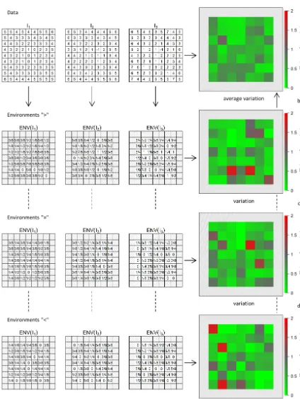
In addition to the overall persistency, the temporal dynamics of local LST patterns are investigated using a second type of “moving window” approach. To analyze the spatial rela-tionship of each pixel within its local neighborhood, for each pixelPcwithin an image a square windoww (the environ-ment) of a defined size (e.g., 3×3 px) around this centralPc is compared to the value ofPc. The environment information (ENV) is summarized to statistical information in the form of percentages of values within the square window that are big-ger than, smaller than or equal to the value ofPc(see Fig. 5a for an example analysis of values that are bigger thanPc).

The variations of the ENV information over time were analyzed for the 28 LST images via the spatial assessment of the coefficient of variation (|σ/µ|) for each of the three setups (<,=, >; see example in Fig. 5c–d). The three spa-tially distributed coefficients of variation are finally reduced to an average pattern of coefficients of variation by taking the mean value of the three setups (Fig. 5b, right).

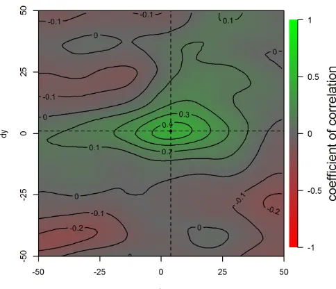
Figure 4. Coefficient of correlation for the LST time series data. The mean coefficient of correlation for all 756 combinations shows a centered behavior (single peak area with maximum correlation of 0.47; green) with a low shift (4,1) within a maximum range of [−50,+50]in bothxandydirection. The size of the correlation window is 51×51 px for 5 fixed, non-overlapping positions (

24 1

2

Figure 4: Coefficient of correlation for the LST time series data. The mean coefficient of 3

correlation for all 756 combinations shows a centered behavior (single peak area with 4

maximum correlation of 0.47; green) with a low shift (4,1) within a maximum range of [-5

50,+50] in both x- and y-direction. The size of the correlation window is 51×51 px for 5 fixed, 6

non-overlapping positions ( ) throughout the images. 7

8

) throughout the images.

The analysis of the LST time series using a window size of 15×15 px=225×225 m2identifies relatively low coef-ficients of variation (Fig. 6) with 90 % of the values between 0.19 and 0.55, 50 % within the range of 0.27 and 0.42, and only 0.03 % of the values larger than 1. This indicates a high local pattern persistency.

Based on both, global and local persistency analysis, rel-atively stationary patterns at the catchment scale, accom-panied by stationary dynamics at the scale of hill slopes throughout the catchment can be expected. The existence of LST pattern persistence also suggests some structured con-trol on LST by some land surface characteristics. In the fol-lowing section possible controls will be extracted and ana-lyzed.

3.3 Principle component analysis

Applying principle component analysis (PCA; for a full mathematical description, see Richards and Jia (2006; chapter 6.1)), or empirical orthogonal functions (EOFs; e.g., Denbo and Allen, 1984; Hamlington et al., 2011; Lorenz, 1956) allows the assessment of independent struc-tures within complex data sets. Because both approaches share a similar methodology, here, PCA is used to determine which spatial factors are controlling patterns of LST within the time series. PCA uses orthogonal transformation to calcu-late a composition of linearly uncorrecalcu-lated values of decreas-ing dominance from possibly correlated monitored variables.

In remote sensing, PCA is often applied to reduce the num-ber of (correlated) variables within classification procedures (see, e.g., Crósta et al., 2003; Moore et al., 2008, for the anal-ysis of multi-spectral, single temporal TIR data to assess dif-ferent geological structures).

Here, the aim is to transform the observed 28 LST patterns into patterns of virtual and independent principal compo-nents. These components represent the most dominant con-trolling factors for the temporal dynamics of LST pattern in decreasing order. An illustrative example for a PCA applica-tion in this context is given in Fig. 7 for artificial data.

The PCA application for the ASTER TIR time series pro-duced 28 independent components as summarized in Ta-ble 1. By construction, components with higher (lower) de-gree show less (more) information and more (less) noise. 61.9 % of the variation is cumulatively expressed via the first five components (third row), while still more than 3 % of the variance are expressed by particular components (second row). In the following, a focus is given to the first five com-ponents (Fig. 9).

Figure 8 illustrates a distinct degree of structured hetero-geneity for these five components. In principle the patterns of the PCs would allow to classify the catchment or land-scape into different functional units that, when using LST images, would strongly reflect the functioning of the land-scape related to the water and energy balance under radiation driven conditions. The number of PCs to be considered in such a classification would depend on the overall number of units that should be differentiated (which will strongly de-pend on computational resources available to explicitly rep-resent within catchment variability), but also on the (cumula-tive) percentage of explained variance of the PCs, as well as on the distribution or, at least, range of the component values of each individual PC.

However, while this is an important topic related to land surface hydrological modeling, the focus here will be on the relationship of the extracted PCs with other land surface characteristics. Given the controls of LST as discussed in the introduction, it is expected to find some relationship of the first dominant PCs with vegetation, soil, geology, elevation, slope, aspect or others. A comparison of the PCs with avail-able data suggested a strong relationship between PC1 and land use data, as well as PC2 with geological information. These relationships are illustrated in Fig. 9, where maps of PC1 and Corine land cover as well as PC2 and a geological map of the Attert catchment are shown next to each other.

B. Müller et al.: Identification of catchment functional units 5351

Figure 5a. Analysis of the coefficient of variation via an “environment assessment” for a designed data set. The data are generated in the same way as in the previous analysis (see Fig. 3). Subfigure (a) illustrates the derivation of a single summary value for the central pixelPc (blue) from the data of the surrounding environmentw(red). The example here investigates how many values within the environment are larger than the central value. This is repeated for all image pixels (except for boundary pixels), resulting in the rightmost picture.

Table 1. Overview on the 28 calculated principle components (PCs) regarding their accounted proportion of variance. In each column, the components show their specific standard deviation (σ), proportion of variance (prop. of VAR) and cumulative proportion of variance (cum. prop.).

PC1 PC2 PC3 PC4 PC5 PC6 PC7

σ 3.475 1.502 1.018 1.006 0.977 0.874 0.867 prop. of VAR 0.431 0.081 0.037 0.036 0.034 0.027 0.027 cum. prop. 0.431 0.512 0.549 0.585 0.619 0.646 0.673

PC8 PC9 PC10 PC11 PC12 PC13 PC14

σ 0.843 0.834 0.792 0.754 0.746 0.730 0.713 prop. of VAR 0.025 0.025 0.022 0.020 0.020 0.019 0.018 cum. prop. 0.699 0.723 0.746 0.766 0.786 0.805 0.823

PC15 PC16 PC17 PC18 PC19 PC20 PC21

σ 0.712 0.694 0.671 0.669 0.646 0.619 0.598 prop. of VAR 0.018 0.017 0.016 0.016 0.015 0.014 0.013 cum. prop. 0.841 0.858 0.875 0.891 0.905 0.919 0.932

PC22 PC23 PC24 PC25 PC26 PC27 PC28

σ 0.589 0.575 0.555 0.535 0.525 0.483 0.357 prop. of VAR 0.012 0.012 0.011 0.010 0.010 0.008 0.005 cum. prop. 0.944 0.956 0.967 0.977 0.987 0.995 1.000

values for forests. In this way, PC1 might be interpreted as related to similar dynamics in leaf area index (LAI; see As-ner et al., 2003), and therefore the potential for water vapor and energy exchange between the land surface and the atmo-sphere. The high values for “mineral extraction” can be ex-plained, as the single, relatively small area is surrounded by forests and partially replanted with smaller trees or shrubs during the observed time span.

When analyzing the component values of PC2 for the dif-ferent geological classes, schist areas show distinct, difdif-ferent distributions compared to the other (mainly) sandstone areas. Schists with a high proportion of fractures are known for a high water drainage potential compared to the remaining

sedimentary geology classes (see Chiang, 1971). The avail-ability of water for transpiration and therefore the splitting of available energy into sensible and latent heat fluxes, resulting in different land surface temperatures, are thereby strongly affected. In this sense, PC2 can be interpreted as being re-lated to bedrock information or coupled soil texture.

B. Müller et al.: Identification of catchment functional units 5353

Table 2. Loadings of the first five components (rows) to reproduce the LST time series (columns). The weights differ largely between the time steps. The lowest coefficient of variation for the loadings is calculated for PC1 (0.195); the highest value for PC2 (136.996). PC3, PC4 and PC5 have coefficients of variation of 80.131, 21.914 and 14.193.

Loading of 25 Feb 2001 23 Sep 2001 15 Feb 2003 21 Mar 2003 3 Aug 2003 15 Apr 2004 17 May 2004

PC1 −0.055 −0.056 −0.044 −0.054 −0.052 −0.038 −0.048

PC2 −0.050 −0.038 −0.099 0.012 0.026 0.054 0.023

PC3 0.045 0.006 0.042 0.041 −0.043 0.099 0.057

PC4 −0.066 −0.072 −0.013 −0.054 −0.055 0.009 0.029

PC5 0.059 0.000 0.075 0.016 −0.018 −0.028 −0.098

24 May 2004 27 May 2005 12 Sep 2006 1 May 2007 15 Jul 2008 24 Jul 2008 26 Sep 2008

PC1 −0.056 −0.043 −0.054 −0.049 −0.061 −0.053 −0.055

PC2 0.002 −0.015 0.019 0.045 −0.025 −0.024 0.004

PC3 0.038 0.014 −0.022 −0.024 −0.036 −0.048 −0.022

PC4 0.008 0.041 −0.063 0.006 0.028 0.014 −0.070

PC5 −0.103 −0.085 −0.026 −0.016 −0.011 −0.001 0.004

21 Mar 2009 20 Apr 2009 22 May 2009 23 Jun 2009 2 Jul 2009 27 Jul 2009 16 Apr 2010

PC1 −0.059 −0.038 −0.050 −0.043 −0.042 −0.049 −0.034

PC2 0.026 0.026 −0.041 −0.028 −0.037 −0.033 0.098

PC3 −0.004 0.010 0.007 −0.067 −0.052 −0.022 0.010

PC4 −0.011 0.091 0.061 0.078 0.112 0.008 0.020

PC5 0.042 0.075 0.007 0.049 0.000 −0.006 0.104

23 Apr 2010 23 Sep 2010 19 Apr 2011 30 May 2011 6 Nov 2011 27 Mar 2012 14 May 2012

PC1 −0.037 −0.034 −0.059 −0.059 −0.028 −0.032 −0.048

PC2 0.070 0.057 −0.024 −0.003 −0.117 0.066 0.017

PC3 0.056 −0.128 −0.035 −0.026 0.069 0.038 0.013

PC4 0.027 −0.061 0.031 −0.041 −0.025 −0.010 0.044

PC5 0.022 0.010 −0.014 −0.043 0.038 0.058 −0.013

Figure 6. Coefficient of variation for the LST time series data. The median coefficient of variation is 0.34, the mean value 0.35. In all, 90 % of the calculated values are within the range of 0.19 and 0.55 (red lines), 50 % are within the range of 0.27 and 0.42 (red dashes) and 0.03 % of the values are larger than 1 (blue arrow).

part of a possible elevation effect might be “hidden” in PC2 already. However, for other more mountainous areas, possi-ble relationships might be more pronounced and should be considered and analyzed in detail.

In addition to the component values, PCA also provides information on the weight of each component within each single time step through calculation of the specific loadings. Table 2 illustrates the first five components and their load-ings for the analyzed data set. While some dependencies of the sign, mean and standard deviation of the loadings with meteorological or hydrological conditions or states in the Attert catchment are expected, here, only the differences in the loadings at individual dates are used to identify a limited number of images that are most distinct in their information content but that represent the wide range of LST dynamics over the considered time period. Based on the cumulative Euclidean distance of loadings within the LST time series, a number of 5 exemplary images are selected for further anal-ysis (15 February 2003, 17 May 2004, 24 May 2004, 27 May 2005 and 27 March 2012).

3.4 Behavioral measure

Figure 7. Principle component analysis for a designed data set. The data are the same as those for Fig. 5. The first row shows the pattern of the original data (I1–I3), the second row shows the three resulting principle components (PC1–PC3). The PCs are scaled to the same numeric domain as the original data and colored alike (orange for low values; green for high values). PC1 shows the dominance of the concentric pattern, explaining 90.5 % of overall variance of the data. PC2 and PC3 are more homogeneous and describe the noise of the construction of the data set.

Figure 8. The first five components of the PCA for the LST time series data.

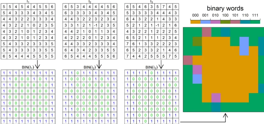
dynamics persistency, the vast data variability is transformed into simple information. Using the five most different im-ages and therefore time steps (see Sect. 3.3), the data are bi-narized using an approach suggested by Hauhs and Lange (2008). The pixels of each image within the time step are separated into values larger than the median value of the im-age (1) or lower (0) (Fig. 11, left). The set of five binarized images can be aggregated into five-letter “words” (Hauhs and Lange, 2008) by concatenating these binary values (see the

three-letter example in Fig. 11; right). The order of letters within the words represents the response of the land surface to differences in the water and energy balance for each pixel. These different land surface responses refer to differently be-having landscape units.

dis-B. Müller et al.: Identification of catchment functional units 5355

Figure 9. The first and second component of the PCA for the LST time series data (left) next to the patterns of the illustration of Corine land cover and geology data (right) of the Attert catchment.

Figure 10. Comparison of component values and spatial information for the Attert catchment. The density distribution of the component values (PC1 in (a); PC2 in (b)) are shown for the different classes of the spatial data sets (Corine land cover in (a); geology in (b)). Mean values of the distributions are shown as vertical bars on the bottom line.

tances, indicating different response of the land surface to-wards radiation-driven conditions; other areas behave very similarly over larger spatial extent. These larger clusters are characterized by a constant behavior throughout the subset time series with short interruptions only (e.g., class “00010” only has one short “break” of length 1). Different binary words represent different land surface functioning and there-fore allow the delineation of functional units (with a focus

Figure 11. Construction of “binary word” classification for a designed data set. The data are the same as those for Fig. 5. On the left, the three images are binarized (BIN) from the upper to the lower panel. Values larger than the median are converted to 1 (blue), values lower are converted to 0 (green). The right panel shows the aggregated words for the three data sets. Not every possible occurrence of words is produced (maximum: 23= 8).

4 Conclusions

An alternative way of characterizing land surface functional-ity based on time series of thermal remote sensing images is introduced. Firstly, it is shown that the overall LST patterns of the time series are spatio–temporally persistent. Secondly, dominant patterns within the time series were extracted via PCA and could be related to physical ecological features, such as land use and geology. Based on these analyses, rep-resentative images from the time series were selected to ex-press land surface functionality in terms of binary words and to classify land surface into different functional units that, again, could be related to existent land use patterns in the catchment. In contrast to the “classical” HRU delineation process – in which maps of land surface properties (DEM, land use, soil) that are often generalized, estimated, outdated or interpolated from sparse measures, are intersected, and hy-drological similarity is assumed for these units – the derived principal components and values, as well as the classification with regards to binary words, both represent “real” and “on-site” catchment functional behavior with regards to LST and therefore to the water and energy balance at each location.

While ASTER data were used here, this approach is appli-cable to any other platform or sensor providing LST informa-tion (e.g., Landsat 8 data, 100 m resoluinforma-tion, TIR). Given the maximum spatial resolution of ca. 100 m in TIR remote sens-ing, any analysis concerning the size of functional similarity in the landscape is limited to that resolution. Aircraft-based TIR sensing might overcome this limitation, but it is still not routinely available yet. More global hence coarse pat-terns can be derived from geostationary satellites (e.g.,

Me-teosat) and might improve spatial representations of global standard data sets for climate modeling; e.g., the FAO (Food and Agriculture Organization of the United Nations) world soil map. By investigating the PCA results for different res-olutions, it should also be possible to develop new statistical up and down scaling methods for model parameterizations. This approach is also limited by the number and seasonal-ity of available (and almost cloud free) LST images. For the Attert catchment, a data set of 28 LST images was available for a period of ca. 12 years. Using the full data set, any sig-nificant land surface changes related to LST are implicitly contained and expressed in the derived principal components and their values, as well as in the derived classification of functional units using binary words. An analysis of historic Landsat images has shown that the land use changes in the Attert catchment have been minimal over the last 35 years, so crop rotation by farmers is the most dominant change over the seasons here. Given an average of not even three avail-able images per year for this mid-latitude region (see Fig. 2), any application of this approach will have to balance between sufficient temporal coverage in order to capture the relevant LST dynamics of the landscape, and not covering too many externally driven changes in the procedure.

land-B. Müller et al.: Identification of catchment functional units 5357

Figure 12. Behavioral classification of the subset LST time series data. The algorithm is producing 25= 32 classes of different frequency. The image shows the full bandwidth with classes named in the legend.

scape functioning with regards to LST. This might change with more complex landscapes. The application of digital numbers instead of extracted LST also showed almost iden-tical results, so that a proper conversion to LST is, in our opinion, not fundamentally needed.

What are the additional benefits of the LST analysis pre-sented here? The analysis of binary words, as prepre-sented in Sect. 3.4, provides a classification of the catchment into ar-eas that behave similarly (with regards to the complex in-teractions of the water and energy balance, as expressed in LST) in terms of response to radiation-driven conditions. These units can either be used in an already-established HRU framework or can provide some guidance on the size of spa-tial discretization of the landscape in land surface model-ing exercises. They might support effective observation and monitoring strategies under limited resources by providing distributed information of distinct behavior and hence might be used as decision support on the spatial distributions of field experiments. The strongest impact of the approach pre-sented is expected when the derived component values from the PCA analysis will be incorporated into model parameter regionalization schemes (e.g., the multi-scale parameter re-gionalization (MPR) scheme presented by Samaniego et al.,

Acknowledgements. We thank the German Research Foundation

(DFG) for funding this research through the CAOS (Catchments as Organised, see CAOS reference below (marked) Systems) Research Unit (FOR 1598; grant no. SCHU1271/5-1). We also want to thank the LPDAAC (Land Processes Distributed Active Archive Center) for providing free ASTER data, as well as the editor and anonymous referees for their contributions to improve this article.

Edited by: H. Cloke

References

Arnold, J. G., Srinivasan, R., Muttiah, R. S., and Williams, J. R.: Large area hydrologic modeling and assessment Part I: Model development, J. Am. Water Resour. As., 34, 73–89, doi:10.1111/j.1752-1688.1998.tb05961.x, 1998.

Asner, G. P., Scurlock, J. M. O., and Hicke, J. A.: Global synthe-sis of leaf area index observations: implications for ecological and remote sensing studies, Global Ecol. Biogeogr., 12, 191–205, doi:10.1046/j.1466-822X.2003.00026.x, 2003.

Beven, K. J. and Kirkby, M. J.: A physically based, variable contributing area model of catchment hydrology, Hydrological Sciences Bulletin, 24, 43–69, doi:10.1080/02626667909491834, 1979.

Bolle, H.-J., Feddes, R. A., and Kalma, J. D. (Eds.): Exchange pro-cesses at the land surface for a range of space and time scales, in: Proceedings of Symposium J3.1, Joint Scientific Assembly of IAMAP and IAHS, Yokohama, Japan, 11–23 July 1993, 626 pp., 1993.

CAOS: CAOS – Catchments as Organised Systems, available at: http://www.caos-project.de (last access: 22 May 2014), 2014. CESSLU: How to calculate reflectance and temperature

us-ing ASTER data, prepared by Abduwasit Ghulam, Cen-ter for Environmental Sciences at Saint Louis University, available at: http://www.gis.slu.edu/RS/ASTER_Reflectance_ Temperature_Calculation.php (last access: 22 May 2014), 2009. Chiang, S. L.: A runoff potential rating table for soils, J. Hydrol.,

13, 54–62, doi:10.1016/0022-1694(71)90200-9, 1971.

Crósta, A. P., De Souza Filho, C. R., Azevedo, F., and Brodie, C.: Targeting key alteration minerals in epithermal deposits in Patagonia, Argentina, using ASTER imagery and principal component analysis, Int. J. Remote Sens., 24, 4233–4240, doi:10.1080/0143116031000152291, 2003.

Denbo, D. W. and Allen, J. S.: Rotary empirical orthog-onal function analysis of currents near the Oregon coast, J. Phys. Oceanogr, 14, 35–46, doi:10.1175/1520-0485(1984)014<0035:REOFAO>2.0.CO;2 1984.

EEA: CORINE Land Cover Project, published by Commission of the European Communities, available at: http://www.eea.europa. eu/publications/COR0-landcover (last access: 22 May 2014), 1995.

EEA: Environmental Terminology and Discovery Service (ETDS), published by European Environment Agency, available at: http://glossary.eea.europa.eu/terminology/concept_html?term= corine%20land%20cover (last access: 22 May 2014), 2014.

Eldeiry, A. and Garcia, L.: Comparison of ordinary kriging, regres-sion kriging, and cokriging techniques to estimate soil salinity using LANDSAT images, J. Irrig. Drain. E.-ASCE, 136, 355– 364, doi:10.1061/(ASCE)IR.1943-4774.0000208, 2010. Elder, T. and Strong, J.: The infrared transmission of

atmo-spheric windows, J. Franklin I, 255, 189–208, doi:10.1016/0016-0032(53)90002-7, 1953.

EPA: Multi-Resolution Land Characteristics Consortium (MRLC), available at: http://www.epa.gov/mrlc/ (last access: 22 May 2014), 2007.

Farah, H. O. and Bastiaanssen, W. G. M.: Impact of spatial varia-tions of land surface parameters on regional evaporation: a case study with remote sensing data, Hydrol. Process., 15, 1585– 1607, doi:10.1002/hyp.159, 2001.

Farr, T. G., Rosen, P. A., Caro, E., Crippen, R., Dure, R., Hens-ley, S., Kobrick, M., Paller, M., Rodriguez, E., Roth, L., Seal, D., Shaffer, S., Shimada, J., Umland, J., Werner, M., Oskin, M., Bur-bank, D., and Alsdorf, D.: The shuttle radar topography mission, Rev. Geophys., 45, RG2004, doi:10.1029/2005RG000183, 2007. Flügel, W. A.: Delineating Hydrological Response Units (HRUs) by GIS analysis for regional hydrological modelling using PRMS/MMS in the drainage basin of the River Bröl, Germany, Hydrol. Process., 9, 423–436, doi:10.1002/hyp.3360090313, 1995a.

Flügel, W. A.: Hydrological Response Units (HRUs) to pre-serve basin heterogeneity in hydrological modelling using PRMS/MMS – case study in the Bröl basin, Germany, in: Mod-elling and Management of Sustainable Basin-Scale Water Re-source Systems, Boulder, Colorado, USA, 1–14 July 1995, 79– 87, 1995b.

Fujisada, H.: Design and performance of ASTER instru-ment, in: Advanced and Next-Generation Satellites, Proceed-ings of SPIE, Paris, France, 15 December 1995, 16–25, doi:10.1117/12.228565, 1995.

Hamlington, B. D., Leben, R. R., Nerem, R. S., Han, W., and Kim, K. Y.: Reconstructing sea level using cyclostationary empirical orthogonal functions, J. Geophys. Res.-Oceans, 1978–2012, 116, doi:10.1029/2011JC007529, 2011.

Hauhs, M. and Lange, H.: Classification of runoff in headwater catchments: a physical problem?, Geography Compass, 2, 235– 254, doi:10.1111/j.1749-8198.2007.00075.x, 2008.

Hirschmüller, H., Innocent, P. R., and Garibaldi, J.: Real-time correlation-based stereo vision with reduced border errors, Int. J. Comput. Vision, 47, 229–246, doi:10.1023/A:1014554110407, 2002.

Hook, S. J., Vaughan, R. G., Tonooka, H., and Schladow, S. G.: Absolute radiometric in-flight validation of mid infrared and thermal infrared data from ASTER and MODIS on the terra spacecraft using the Lake Tahoe, CA/NV, USA, automated validation site, IEEE T. Geosci. Remote, 45, 1798–1807, doi:10.1109/TGRS.2007.894564, 2007.

Kheir, R. B., Greve, M. H., Bøcher, P. K., Greve, M. B., Larsen, R., and McCloy, K.: Predictive mapping of soil organic carbon in wet cultivated lands using classification-tree based models: the case study of Denmark, J. Environ. Manage., 91, 1150–1160, doi:10.1016/j.jenvman.2010.01.001, 2010.

re-B. Müller et al.: Identification of catchment functional units 5359

view, precision agriculture, 11, 82–100, doi:10.1007/s11119-009-9123-3, 2010.

Lagacherie, P., Bailly, J. S., Monestiez, P., and Gomez, C.: Using scattered hyperspectral imagery data to map the soil properties of a region, Eur. J. Soil Sci., 63, 110–119, doi:10.1111/j.1365-2389.2011.01409.x, 2012.

Lorenz, E. N.: Empirical orthogonal functions and statistical weather prediction, Scientific Report No. 1, Statistical Forecast-ing Project, Department of Meteorology, MIT, 49 pp., 1956. Moore, F., Rastmanesh, F., Asadi, H., and Modabberi, S.:

Map-ping mineralogical alteration using principal-component analy-sis and matched filter processing in the Takab area, north-west Iran, from ASTER data, Int. J. Remote Sens., 29, 2851–2867, doi:10.1080/01431160701418989, 2008.

Moran, M. S.: Thermal infrared measurement as an indicator of plant ecosystem health, in: Thermal Remote Sensing in Land Surface Processes, edited by: Quattrochi, D. A. and Luvall, J., CRC Press, Boca Raton, Florida, USA, 257–282, doi:10.1201/9780203502174-c9, 2004.

Mulder, V. L., de Bruin, S., Schaepman, M. E., and Mayr, T. R.: The use of remote sensing in soil and terrain mapping – a review, Geoderma, 162, 1–19, doi:10.1016/j.geoderma.2010.12.018, 2011.

NASA: Shuttle Radar Topography Mission, available at: http:// www2.jpl.nasa.gov/srtm (last access: 22 May 2014), 2009. Neumann, L. N., Western, A. W., and Argent, R. M.: The

sensitiv-ity of simulated flow and water qualsensitiv-ity response to spatial het-erogeneity on a hillslope in the Tarrawarra catchment, Australia, Hydrol Proc., 24, 76–86, doi:10.1002/hyp.7486, 2010.

Pomeroy, J. W., Gray, D. M., Brown, T., Hedstrom, N. R., Quin-ton, W. L., Granger, R. J., and Carey, S. K.: The cold regions hydrological model: a platform for basing process representation and model structure on physical evidence, Hydrol. Process., 21, 2650–2667, doi:10.1002/hyp.6787, 2007.

Richards, J. A. and Jia, X.: The principal components transforma-tion, in: Remote Sensing Digital Image Analysis: an Introduc-tion, 4th Edn., Springer, Berlin, Germany, 133–148, 2006. Samaniego, L., Kumar, R., and Attinger, S.: Multiscale

pa-rameter regionalization of a grid-based hydrologic model at the mesoscale, Water Resour. Res., 46, W05523, doi:10.1029/2008WR007327, 2010.

Serbin, G., Daughtry, C. S. T., Hunt, E. R., Jr., Reeves III, J. B., and Brown, D. J.: Effects of soil composition and mineralogy on remote sensing of crop residue cover, Remote Sens. Environ., 113, 224–238, doi:10.1016/j.rse.2008.09.004, 2009a.

Serbin, G., Hunt, E. R., Jr., Daughtry, C. S. T., McCarty, G. W., and Doraiswamy, P. C.: An improved ASTER index for re-mote sensing of crop residue, Rere-mote Sensing, 1, 971–991, doi:10.3390/rs1040971, 2009b.

SGL: Carte Géologique du Luxembourg, Feuille No. 7, Redange, 1:25 000, R. Colpach, Service Géologique du Luxembourg, Lux-embourg, 2003.

Srinivasan, R., Ramanarayanan, T. S., Arnold, J. G., and Bed-narz, S. T.: Large area hydrologic modeling and assessment, Part II: Model application, J. Am. Water Resour. As., 34, 91–101, doi:10.1111/j.1752-1688.1998.tb05962.x, 1998.

Steenpass, C., Vanderborght, J., Herbst, M., Simunek, J., and Vereecken, H.: Estimating soil hydraulic properties from infrared measurements of soil surface temperatures and TDR data, Va-dose Zone J., 9, 910–924, doi:10.2136/vzj2009.0176, 2010. Summers, D., Lewis, M., Ostendorf, B., and Chittleborough, D.:

Unmixing of soil types and estimation of soil exposure with sim-ulated hyperspectral imagery, Int. J. Remote Sens., 32, 6507– 6526, doi:10.1080/01431161.2010.512931, 2011.

Taiz, L. and Zeiger, E.: Plant Physiology, 5th Edn., Sinauer Asso-ciates, Sunderland, Massachusetts, USA, 782 pp., 2010. Zehe, E., Ehret, U., Pfister, L., Blume, T., Schröder, B., Westhoff,