https://doi.org/10.5194/hess-23-4397-2019 © Author(s) 2019. This work is distributed under the Creative Commons Attribution 4.0 License.
A review of methods for measuring groundwater–surface
water exchange in braided rivers
Katie Coluccio1and Leanne Kaye Morgan1,2
1Waterways Centre for Freshwater Management, University of Canterbury,
Private Bag 4800, Christchurch 8140, New Zealand
2College of Science and Engineering, Flinders University, G.P.O. Box 2100, Adelaide SA 5001, Australia
Correspondence:Katie Coluccio (katie.coluccio@pg.canterbury.ac.nz) Received: 12 November 2018 – Discussion started: 17 December 2018
Revised: 5 September 2019 – Accepted: 23 September 2019 – Published: 29 October 2019
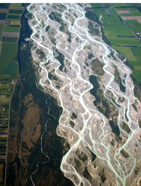
Abstract. Braided rivers, while uncommon internationally, are significant in terms of their unique ecosystems and as vi-tal freshwater resources at locations where they occur. With an increasing awareness of the connected nature of surface water and groundwater, there have been many studies exam-ining groundwater–surface water exchange in various types of waterbodies, but significantly less research has been con-ducted in braided rivers. Thus, there is currently limited un-derstanding of how characteristics unique to braided rivers, such as channel shifting, expanding and narrowing mar-gins, and a high degree of heterogeneity affect groundwater– surface water flow paths. This article provides an overview of characteristics specific to braided rivers, including a map showing the regions where braided rivers are mainly found at the global scale: Alaska, Canada, the Japanese and Euro-pean Alps, the Himalayas, Russia, and New Zealand. To the authors’ knowledge, this is the first map of its kind. This is followed by a review of prior studies that have investigated groundwater–surface water interactions in braided rivers and their associated aquifers. The various methods used to char-acterise these processes are discussed with emphasis on their effectiveness in achieving the studies’ objectives and their applicability in braided rivers. We also discuss additional methods that appear promising to apply in braided river set-tings. The aim is to provide guidance on methodologies most suitable for future work in braided rivers. In many cases, previous studies found a multi-method approach useful to produce more robust results and compare data collected at various scales. Given the challenges of working directly in braided rivers, there is considerable scope for the increased use of remote sensing techniques. There is also opportunity
for new approaches to modelling braided rivers using inte-grated techniques that incorporate the complex river bed ter-rain and geomorphology of braided rivers explicitly. We also identify a critical need to improve the conceptual understand-ing of hyporheic exchange in braided rivers, rates of recharge to and from braided rivers, and historical patterns of dry and low-flow periods in these rivers.
1 Introduction
bod-ies and, conversely, surface water recharge to groundwater. These questions can be considered at various spatial and tem-poral scales (Fleckenstein et al., 2010; González-Pinzón et al., 2015; Magliozzi et al., 2018).
This paper often refers to groundwater–surface water ex-change, which in this context may include regional ground-water exchange with river ground-water, as well as hyporheic zone exchange. The hyporheic zone consists of the sediments sur-rounding a river that are permeated by stream water (Boano et al., 2014). Hyporheic flow consists of river water that en-ters the hyporheic zone and re-emerges at the surface at some location downstream (Boano et al., 2014). Groundwater may also mix with surface water in the hyporheic zone (Boano et al., 2014). Hyporheic zone flow is multi-directional and may occur at multiple temporal and spatial scales (Carde-nas, 2015). It is critical to note that there have been very few studies examining the hydrology and conceptualisation of the hyporheic zone in braided rivers. This is a crucial gap in knowledge, as this often limits our ability to interpret data collected from braided rivers relating to groundwater–surface water exchange.
This article investigates the methods that have previously been used for examining groundwater–surface water ex-change in braided rivers and discusses scope for new meth-ods to be applied. Braided rivers are a highly dynamic type of river with meandering channels, wide bars and vari-able flow levels. Globally, braided rivers are relatively rare; they are mainly found in the Canadian Rockies, Alaska, the Himalayas, New Zealand, Russia, and the European and Japanese Alps (Fig. 1) (Tockner et al., 2006; Alexeevsky et al., 2013). There are instances of braided rivers at loca-tions outside of these regions (e.g. the US, Scotland, Iceland, China, Poland, Belarus, Colombia, Congo, Brazil, Paraguay, Argentina, and the Touat Valley in Africa); however, these lo-cations are not shown in Fig. 1 because, at a global scale, they are not where braided rivers are mainly found. The regions displayed in Fig. 1 are regularly cited in literature on braided rivers as the main regions where this river type can be found (Hibbert and Brown, 2001; Tockner et al., 2006). Braided rivers generally occur in mountainous areas with a large sed-iment source (such as glacial outwash), high river discharge rates and a steep topographic gradient (Charlton, 2008). These high-energy environments enable the rivers to carry large sediment loads. When these rivers reach their capacity to carry sediment, they form gravel braids, which branch out and re-join, creating gravel islands and shallow bars (Figs. 2 and 3). Bars and islands are often referred to as distinct fea-tures, with bars existing at periods of low flow, while islands are generally more permanent features that may be vegetated (Charlton, 2008). Braided rivers can completely change their geometry over a few decades. They undergo expansion and contraction phases in which their channels widen or narrow, depending on sediment supply and river flows (Piégay et al., 2006). The wetted channels of the river can shift, abandoning channels and re-occupying old channels (Charlton, 2008).
Relatively erodible streambanks, which allow for wide chan-nels to form and meander, are a key characteristic of braided rivers. These rivers generally have gravel beds but sand-bed rivers such as the Brahmaputra–Jamuna, which begins in the Himalayas and flows through India and Bangladesh (and is the world’s largest braided river), can also form braided pat-terns (Sarker et al., 2014). The Brahmaputra–Jamuna is the only braided river in this review that is not a gravel-bed braided river. Also, it is important to note, the specific rivers discussed in this article are all braided rivers unless otherwise mentioned.
Braided river deposits have formed extensive aquifers throughout the world including many in the regions shown in Fig. 1 (Brown, 2001; Huggenberger and Regli, 2006). The complex depositional processes of braided rivers create heterogeneous aquifer properties (Huggenberger and Regli, 2006), and a significant portion of flow occurs at varying scales in preferential flow paths formed by previous river flow channels (Close et al., 2014; Dann et al., 2008; White, 2009). The complexity of braided rivers and their underly-ing heterogeneous aquifers makes managunderly-ing these systems in an integrated manner, that accounts for surface water-groundwater interaction, challenging. For example, there is significant uncertainty surrounding rates of groundwater recharge from large braided rivers in New Zealand, which complicates the sustainable allocation of water extraction rights from surface water and groundwater sources (Close et al., 2014). There is also limited knowledge of how hyporheic flow processes operate and how they impact river flow levels and water quality in braided rivers. Braided rivers also of-ten have reaches that become dry or have very low flows at the surface. The historical patterns of these drying and low-flow periods, and the impact of groundwater–surface water exchange on this, is an area of research where improved knowledge is needed. For example, many irrigation schemes have artificially raised groundwater levels due to land surface recharge, or lowered groundwater levels due to abstraction in comparison to their pre-irrigation states. In some rivers this has affected their losing/gaining patterns (Burbery and Rit-son, 2010; Riegler, 2012).
Figure 1. Locations where most braided rivers occur globally. Map base layer image attribution: “World Map-A non-Frame” is licensed under CC BY-SA 3.0.
Figure 2.Rakaia River in New Zealand displaying a classic braided pattern. Image reproduced with permission by Andrew Cooper.
and swimming, and as places of outstanding natural charac-ter.
[image:3.612.50.286.289.601.2]However, braided rivers face pressure from many angles. In many places they are subject to damage from vehicles, gravel extraction, invasive plant species, development on
Figure 3.The Rakahuri/Ashley River in New Zealand displaying a typical braided river consisting of multiple channels, gravel bars and vegetated islands. Photo: Katie Coluccio.
river margins, damming, land encroachment, containment through flood engineering, low-flow levels and poor water quality (Caruso, 2006; Larned et al., 2008; Tockner and Stan-ford, 2002). These factors can influence river processes in many ways, including altering the rate of sedimentation or changing the flow regime, which may impact various uses of these rivers, as well as riparian ecosystems (Piégay et al., 2006).
[image:3.612.310.546.289.468.2]studies of small reaches of valley-confined systems (Fergu-son et al., 1992). Beginning in the mid-1990s, there were ad-vances in numerical models to estimate the braiding process in reaches, remote sensing, and the quantification of river morphology and morphological change using digital eleva-tion models (e.g. Bernini et al., 2006; Copley and Moore, 1993; Doeschl et al., 2006; Huggenberger, 1993). This al-lowed, for the first time, the visualisation and analysis of the morphology of large braided rivers (e.g. Hicks et al., 2006; Huggenberger, 1993; Lane, 2006). A number of studies have looked at the surface water features of braided rivers (e.g. Davies et al., 1996; Meunier et al., 2006; Young and War-burton, 1996), as well as aquifers created by braided river deposits (e.g. Huber and Huggenberger, 2016; Pirot et al., 2015; Vienken et al., 2017). However, the connections be-tween the two have been less explored, particularly in regard to hydrology and conceptualisation of the hyporheic zone.
This article addresses this gap in the literature by review-ing methods previously used in braided rivers internation-ally to characterise groundwater–surface water interactions, as well as recommendations for new methods that can be applied in this type of river environment. The objective is to provide guidance for future braided river studies. As de-scribed in this section, braided rivers have many features that may make it difficult to apply techniques used in dif-ferent river environments. While many of these features are found in other river types, they exist in a particular combi-nation in braided rivers, which makes it problematic to in-vestigate groundwater–surface water exchange. The rapidly shifting channels of braided rivers make it difficult to es-tablish, maintain and access study sites. The typical coarse gravel substrate makes it challenging to install instruments in the riverbed. Large braided rivers can be several kilo-metres wide, resulting in data collection across the width of the river being difficult or impossible. The very perme-able gravel streambeds are often highly gaining or losing in respect to groundwater, and these interactions can have large temporal variability. The mixed sand and gravel sub-strate makes it nearly impossible to take undisturbed sam-ples for sediment structure analysis. The heterogeneous na-ture of the river substrate and strucna-tures – largely mixed sand and gravel, with some clay and silt layers, and open frame-work gravels – make upscaling point-scale data difficult. A significant portion of river flow occurs within the streambed; and in aquifers, the open framework gravels (i.e. paleo river channels) serve as preferential flow paths. In relation to the methods used in previous studies, this article examines the equipment and study design, cost, issues of temporal and spa-tial scales, and ultimately the techniques’ effectiveness. For general overviews of methodologies not specific to braided river applications, refer to Kalbus et al. (2006); Brodie et al. (2007); Rosenberry and LaBaugh (2008); Lovett (2015); Rosenberry et al. (2015); and Brunner et al. (2017).
2 Methodologies for assessing groundwater–surface water interactions in braided rivers
Various types of methods have been used to investigate groundwater–surface water exchange in braided rivers such as mass balance approaches; hydrochemical tracers; direct measurement of hydraulic properties; and modelling. Many of these studies employed multiple methods to meet their objectives. To thoroughly and clearly assess each method, the techniques, and their advantages and limitations will be discussed individually in the following section, and the dis-cussion section will review the merits and limitations of multi-method studies. This information is then summarised in Sect. 3.
2.1 Water budgets
Some of the most commonly used methods for identifying gains and losses to braided rivers have been based on a mass balance approach. The underlying principle of this method is that any gain or loss of surface water can be related to the water source, and therefore the groundwater component can be identified and quantified (Kalbus et al., 2006). Many of these mass balance approaches have used water budgets to separate groundwater and surface water components both on river-reach and catchment-wide scales.
regression analysis. White et al. (2012) used a steady-state groundwater budget to estimate groundwater outflow from the riverbed based on the mean daily flow at a recorder site on the Waimakariri River and groundwater level observa-tions in a monitoring well array beside the river. The authors found that river channel area rather than channel position was most important in their calculations; however, they recom-mended that future research examine the effects of channel position and area on groundwater outflow. This is particu-larly relevant in braided rivers, as their channel positions of-ten change. Both Simonds and Sinclair (2002) and Doering et al. (2013) used flow gauging as part of multi-method studies for estimating groundwater–surface water interactions in the Dungeness River (Washington State, US) and Tagliamento River (northeastern Italy), respectively. These authors con-ducted concurrent gauging to calculate the net loss or gain of flow along river reaches and compare to data collected from other methods.
A smaller number of braided river studies (e.g. Burbery and Ritson, 2010) have used catchment-scale water budget calculations to estimate the inflow and outflow from braided river catchments and distinguish groundwater from surface water sources. The underlying relationship is provided below (modified from Scanlon et al., 2002):
inflow=outflow±1S. (1)
Here, inflow is the sum of precipitation, surface water in-flow and groundwater inin-flow. Outin-flow is comprised of ac-tual evapotranspiration, surface water outflow and groundwa-ter outflow.1Sis the change in water storage in the catch-ment. This also considers artificial changes to water levels in the catchment such as industrial discharges to surface wa-ter or wawa-ter abstraction. Burbery and Ritson (2010) calcu-lated a water budget for the Orari River catchment in Canter-bury, New Zealand, which was based on field observations from various methods including flow gauging and groundwa-ter well observations, climate data, and wagroundwa-ter use data. The authors used the flow gauging data to classify gaining and losing reaches in four of the rivers in the catchment. They noted that in order to obtain a greater level of detail about groundwater–surface water connectivity at the local scale, shorter-spaced flow gauging coupled with high-resolution piezometric surveys and aquifer pumping tests should be car-ried out (Burbery and Ritson, 2010).
Advantages and limitations
River-reach water budgets are useful for identifying hotspots of river gains and losses at a broad scale. However, there are several issues regarding their effectiveness in braided rivers. As detailed in Section 1, these types of rivers are typically comprised of heterogeneous materials and thus there may be small-scale interactions of groundwater and surface wa-ter within reaches, which flow gauging is poor at identify-ing (Hughes, 2006). For example, Larned et al. (2015) noted
that lag time calculations can only highlight generalised flow paths, whereas predicting more specific groundwater flow paths or residence times would require studies using addi-tional techniques such as tracers or potentiometric data. Also, accurate measurements of flow rates can be compromised by several factors including interference of macrophytes in the streambed, low flow, imprecise or shifting river margins, high sediment load, or unstable streambeds that permit parafluvial flow (i.e. flow in the area of riverbed that is to some extent annually scoured by flooding; Stanford, 2007). As noted by Close et al. (2014), there is significant uncertainty around estimates of river to groundwater flows solely based on hy-draulic measurements, particularly for large braided rivers, as these environments provide various challenges for accu-rate flow measurements. These systems are difficult to mea-sure because precise flow gauging can only be carried out during low flows and measurement errors can be consider-able (Close et al., 2014). Often the measurement error is greater than the net exchange of groundwater and surface wa-ter (LaBaugh and Rosenberry, 2008).
Catchment water budgets can be a useful method at a larger scale but are generally not appropriate for assessing small-scale groundwater–surface water interactions, as the accuracy of recharge rates to or from rivers is limited by the accuracy of the measurement of the other components in the budget (Scanlon et al., 2002). They can be simple and quick to calculate, but this depends on how time consuming or ex-pensive the data collection is. Also, this method can have low resolution because of the limited number of flow gauging sta-tions on rivers (Kalbus et al., 2006). Thus, when calculating budgets for large catchments, the errors can be significant. 2.2 Hydrochemistry
oxygen (e.g. Larned et al., 2015; Rodgers et al., 2004), sil-ica (e.g. Botting, 2010; Rodgers et al., 2004; Soulsby et al., 2004), nitrate (e.g. Burbery and Ritson, 2010; Larned et al., 2015; White et al., 2012) and sulfate (e.g. Acuña and Tock-ner, 2009; Botting, 2010).
2.2.1 Stable isotopes
Oxygen, which is a key component of water, naturally occurs in three stable isotopic forms: mainly as oxygen-16 (16O), and in smaller proportions as oxygen-17 (17O) and oxygen-18 (18O) (Sharp, 2007). Due to the difference in mass be-tween these isotopes, they undergo fractionation during evap-oration and condensation (Taylor et al., 1989). The pro-cess is largely driven by temperature, humidity and salin-ity, whereby precipitation is increasingly depleted in 18O at colder temperatures (which tend to occur at higher eleva-tions) (Sharp, 2007). The ratio of 16O to 18O (referred to asδ18O) is used to identify the relative concentrations of the two most abundant stable oxygen isotopes. This allows for the identification of groundwater recharged by alpine sources and lowland rainfall (Burbery and Ritson, 2010) and can shed light on groundwater flow paths in aquifers.
Several studies have used δ18O to characterise groundwater–surface water exchange in braided rivers and their associated aquifers. Blackstock (2011) found their isotopic model for the Christchurch, New Zealand, ground-water system matched well with previous physical mass balance calculations and that stable isotope analysis was useful, especially in shallow groundwater. Botting (2010) found that stable isotope analysis was the most effective technique for distinguishing surface water from groundwater amongst the multiple methods that they used (including hydrochemical sampling, pumping tests, and groundwater well observations) in a study of the north bank of the braided Wairau River in New Zealand. In addition, Vincent (2005) successfully used δ18O analysis to identify groundwater recharge sources in the upper Selwyn River catchment. Burbery and Ritson (2010) usedδ18O analysis to determine alpine versus lowland recharge sources for groundwater in the Orari River catchment. Of the various methods used in the study (which also included flow gauging, a catchment-scale water budget, chemical tracers and groundwater level observations), the authors found δ18O analysis to be highly effective for understanding groundwater–surface water interactions in the catchment. Givenδ18O varies seasonally, they recommended sampling be carried out at various times during the year to obtain better temporal resolution, as well as on a long-term basis to consider climatic variations. Hanson and Abraham (2009) carried out δ18O and other hydrochemical analyses along two transects across New Zealand’s Canterbury Plains. The authors found δ18O to be the most reliable tracer to differentiate between land surface recharge and alpine river water. However, they pointed out that a suite of tracers would be needed to characterise
groundwater flow paths and groundwater recharge sources. They also noted thatδ18O can be significantly altered where alpine water is used for irrigation.
2.2.2 Radon
Radon-222 (Rn-222) is another useful tracer for identifying groundwater–surface water interactions. It is a chemically and biologically inert radioactive gas part of the uranium-238 decay process and is present in nearly all rocks and soils (LaBaugh and Rosenberry, 2008). As water flows through rocks and soils it becomes enriched in Rn-222. In surface waters, radon quickly degasses, so groundwater generally has Rn-222 concentrations 3 to 4 orders of magnitude higher than surface waters, thus making it an effective tracer in many en-vironments (Burnett et al., 2001). For example, an area of high radon concentrations in surface water would suggest groundwater inflow. It is a cost-effective, simple technique that is suitable for study areas ranging in size (Martindale, 2015).
Rn-222 analysis can address many questions related to groundwater and surface water interactions. In a multi-method study in the braided Tagliamento River in northeast-ern Italy, Acuña and Tockner (2009) used Rn-222 to assess the residence time of upwelling groundwater in the hyporheic zone. Moore (1997) analysed Rn-222 to estimate groundwa-ter inflow to the Brahmaputra River in the Bay of Bengal. Close et al. (2014) used Rn-222 sampling to calculate the ve-locity of groundwater recharge from the Waimakariri River to groundwater in the Canterbury Plains in New Zealand us-ing the us-ingrowth (i.e. the rate of build-up in a closed system) equation for Rn-222. The authors recommended that a high-resolution study with closely spaced sampling sites could be useful for highlighting preferential flow paths in the ripar-ian zone. In addition, Close (2014) sampled Rn-222 amongst other hydrochemical parameters in the Wairau River in Marl-borough and in groundwater wells within 5 km of the river to better understand the groundwater–surface water interac-tions in the river and the amount and variability of recharge to the groundwater system. Close (2014) found that temperature correlated well with the spatial distribution of the radon but added that there could be significant errors with estimating groundwater flow paths due to local heterogeneity and the meandering nature of the alluvial deposition process in the area. Close (2014) recommended analysing temperature and data collected from piezometers in conjunction with radon to resolve these uncertainties.
discharge and hyporheic zone exchange using radon analy-sis (Lovett, 2015; Martindale, 2015). Rn-222 concentrations will also vary with different mineral compositions in the rocks present (Close et al., 2014).
2.2.3 Chloride
The chloride ion (Cl−) can be used as an indicator for groundwater and surface water mixing in locations with suf-ficiently distinct chloride concentrations in groundwater and surface waters. For example, the groundwater surrounding the Bow River in the Canadian province of Alberta has el-evated levels of chloride from road salting. This allowed Cantafio and Ryan (2014) to measure chloride levels in an urban reach of the river and assess water quality impacts and baseflow sources. They found that nearly all river flow origi-nates in the Rocky Mountains and there is little contribution from groundwater.
Chloride is frequently sampled amongst a suite of hy-drochemical parameters to investigate groundwater and sur-face water interactions, as groundwater often becomes en-riched in chloride as it passes through soil and rocks (Dom-misse, 2006). Burbery and Ritson (2010) measured chlo-ride concentrations in the Orari River catchment in New Zealand, specifically looking at chloride-to-sulfate ratios to delineate groundwater–surface water interactions and exam-ine recharge sources in the catchment. They found that basic ion chemistry was useful for determining the extent of the Orari River water but noted that results can be complicated by hydrochemical changes due to land use activities. Sev-eral other studies measured chloride to determine recharge sources and quantities in braided rivers and their associ-ated aquifers including Acuña and Tockner (2009), Larned et al. (2015), Botting (2010) and Domisse (2006).
2.2.4 Alkalinity
Alkalinity can serve as an effective indicator for determin-ing catchment water sources. In a study of the braided River Feshie, in the Cairngorms in Scotland, Rodgers et al. (2004) used alkalinity as a tracer to investigate temporal changes in stream water hydrochemistry and characterise sources of river flow. The authors noted that Gran alkalinity is partic-ularly useful as it serves as a directly measurable, close ap-proximation to the acid neutralising capacity, which is con-sidered a conservative chemical tracer. Gran plots are com-monly used to determine alkalinity and acid neutralising ca-pacity in water with low alkalinity or low conductivity. A Gran function plot identifies the point at which all alka-linity has been titrated in a strong-acid–strong-base titra-tion (Rounds and Wilde, 2002). Rodgers et al. (2004) used EMMA to estimate different hydrological sources of River Feshie water. The authors were reasonably confident of their estimates because of the extensive temporal and spatial com-ponents of their study. Because of the relative simplicity and
low cost of the Gran alkalinity method, these types of longer-term and detailed spatial surveys are becoming increasingly feasible (Rodgers et al., 2004), though may be costly in terms of human resources required. In another study in the Feshie catchment, Soulsby et al. (2004) conducted a geochemical tracer study to improve large-scale flow path understanding. The authors carried out chemical-based hydrograph separa-tions to separate baseflow from storm event sources. They analysed for Gran alkalinity, which they noted was simple and inexpensive to measure. Alkalinity has proven to be a useful parameter in the United Kingdom (UK) to distinguish between water sourced from acidic, organic soils (which are common in the UK at shallow depths) and deep, older groundwater. Soulsby et al. (2004) found their study pro-vided valuable information at the sub-catchment scale, but more information was needed at finer spatial scales.
Advantages and limitations
Hydrochemistry can provide significant insight into catchment-wide hydrology, as well as provide estimations of seepage flux on the point scale (Close, 2014; Dommisse, 2006; Lovett, 2015). Even considering catchment hetero-geneity, some tracers can behave predictably enough to serve as effective tracers for studies of braided rivers (Soulsby et al., 2004). Environmental tracers are useful in settings where there is a sufficient difference between tracer concentrations in the groundwater and surface water, and some parameters can be easily incorporated in long-term routine monitoring programs. Disadvantages of these methods include that hydrochemistry of the baseflow and storm event water composition may be too similar, or that hydrochemistry may not be constant in time or space (Genereux and Hooper, 1998). Importantly, various tracers such as dissolved oxygen, pH, nitrate and sulfate may be affected by biogeochemical processes, so to be effective, the tracers must be conservative at the scale of the investigation. Also, land use activities may alter hydrochemistry in catchments, for example from fertiliser application or mixing of water sources through irrigation (Soulsby et al., 2004). Additionally, some low tracer concentrations may cause analysis errors (e.g. in the case of radon) (Close, 2014).
2.3 Temperature studies
zones as well as quantify the flux of water moving between groundwater and surface water systems (Andersen, 2005). There are various methods involving temperature sensing that range in complexity, scale and cost. One-off temperature readings can be taken using probes, or sensors and data log-gers can gather time-series data either in-stream or in ground-water wells. Vertical and horizontal temperature profiles can also be measured by arranging sensors in a series either in-stream or in wells on river margins. Temperature profiles can be analysed using various methods such as VFLUX (Gor-don et al., 2012) or the steady-state approach (Schmidt et al., 2006). Some temperature methods, such as thermal infrared imaging and fibre-optic temperature sensing (both of which are discussed further in Sect. 4), are best suited for identify-ing patterns, such as temperature differences in surface wa-ter that may indicate areas of recharge or discharge. Other methods such as temperature depth profiles can be used to quantify the flux of water through the streambed.
The following studies demonstrate various applications of temperature measurement that have been used to characterise groundwater–surface water exchange in braided rivers. Pas-sadore et al. (2015) conducted thermal monitoring to charac-terise the temporal and spatial variability of streambed wa-ter fluxes in the Brenta River in Italy. They used heat as a tracer in conjunction with water level measurements and found this combination of methods to be effective in esti-mating groundwater–surface water interactions. Two studies of the Wairau River in Marlborough, New Zealand, analysed temperature (Close, 2014; Close et al., 2016). Close (2014) measured temperature in the river and in groundwater wells located near the river to characterise river recharge to the aquifer. The author compared the data to Rn-222 analysis and found that the temperatures correlated well with the spa-tial distribution of radon. Close et al. (2016) used the daily mean temperatures in groundwater wells to estimate the lag time between the river and the observation wells. Lastly, Coluccio (2018) used VFLUX to analyse diurnal tempera-ture signals to characterise seepage through the streambed of a braided river. The study determined the direction and mag-nitude of vertical seepage through the streambed using tem-perature probes in the Ashburton River in New Zealand. The results were compared with hydrochemistry and water level measurements in the river and shallow groundwater to bet-ter inform the inbet-terpretation of the temperature data. Coluc-cio (2018) found that it was difficult to distinguish between shallow groundwater and hyporheic flow and also noted that further studies would benefit from combining a point-scale method like temperature probe analysis with broader-scale techniques.
Advantages and limitations
Heat tracers offer many techniques at varying spatial and temporal scales. Broad-scale methods like aerial thermal in-frared imaging can be used to obtain large-scale data, and
they can offer the advantage of remote collection of data in areas that are difficult to access. Point-scale techniques using temperature sensors can indicate surface water-groundwater interactions at a specific location. Some methods of tem-perature analysis can also quantify seepage flux (e.g. us-ing diurnal signal analysis). The methods range in cost and complexity, and thus can be tailored to suit a study’s needs. There are some limitations including that a temperature gra-dient between groundwater and surface water might not al-ways be present (e.g. this may be affected by environmen-tal conditions such as season, wind, shade from vegetation or rapidly changing river levels) (Johnson, 2003). Also, for certain types of analysis, temperature needs to be measured continuously (Irvine et al., 2017). In addition, due to the dy-namic nature of braided rivers and their associated sediments, heat transfer within the heterogeneous materials may be non-linear.
2.4 Darcy approach 2.4.1 Hydraulic gradient
Groundwater levels are often used to aid in the understanding of groundwater–surface water interactions, and there have been several studies conducted in braided rivers using this technique. Groundwater level data can be used to identify the hydraulic gradient (i.e. the difference in hydraulic head over a given distance) at a location, which can reveal groundwater discharge to a river or river recharge into an aquifer. The un-derlying principle is that if groundwater levels in a well are higher than the river level, the river is gaining (i.e. groundwa-ter is flowing into the river). Conversely, where river levels are higher than the groundwater level in a nearby well, the river is losing (i.e. river water is flowing into groundwater). It is worthwhile to note that it is important to obtain a con-ceptual understanding of the relationship of the river to the water table, as the river might be connected, disconnected or in a transitional state between the two (Brunner et al., 2009). Groundwater levels are most typically measured using pres-sure transducers or electronic water level indicators.
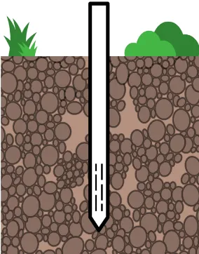
Figure 4. Conceptual diagram of a mini-piezometer (Coluccio, 2018).
Once the hydraulic gradient has been measured, the mag-nitude of groundwater flow into or out of a river can be esti-mated using the Darcy equation:
Q= −KA1h
1l, (2)
whereQ[L3T−1] is the volume of flow,A[L2] is the cross-sectional area perpendicular to flow through which the water passes, and K [L T−1] is hydraulic conductivity (Schwartz and Zhang, 2003). For calculating the horizontal flow magni-tude, a horizontal hydraulic conductivity of the surrounding aquifer is generally used. To calculate the vertical magnitude of flow, the vertical hydraulic conductivity of the streambed needs to be determined, as does the streambed area over which the water exchange occurs (Simonds and Sinclair, 2002).
In terms of specific methods that can be used for mea-surements, existing piezometers (i.e. monitoring wells) near rivers can be useful for conducting these types of stud-ies, particularly given the often high cost of drilling new wells. Please refer to a standard text such as Fetter (2001) for a definition of piezometers. Mini-piezometers, which are scaled-down versions of piezometers and typically installed no deeper than about 2 m (Figs. 4 and 5), have been previ-ously used in studies of braided rivers (Acuña and Tockner, 2009; Doering et al., 2013; Malard et al., 2001). We recom-mend referring to the studies mentioned in this section for piezometer designs for braided river applications, as feasibil-ity of installation into coarse gravel is one of the significant limitations of this technique, and not all designs would be effective in braided rivers for this reason.
[image:9.612.311.546.66.223.2]Previous studies have examined the correlations between groundwater levels and river levels to establish the degree of connectedness of groundwater systems and braided rivers, for example, attempting to identify the causes of drying
Figure 5.Mini-piezometer installed on the bank of a braided river (Coluccio, 2018).
reaches and changes in long-term river flows. Prior studies have been carried out in catchments with substantial agricul-tural surface and/or groundwater abstraction for irrigation. Thus, the questions here are often whether abstraction has caused drying in rivers or decreases in river flows, and what effect future abstraction will have. These studies have of-ten coupled groundwater level measurements with stream-flow gauging and physicochemical sampling of river water and groundwater. Riegler (2012) examined groundwater lev-els, in conjunction with flow gauging, in the North Branch of the Ashburton River in Canterbury, New Zealand, to at-tempt to correlate groundwater levels and decreased flow lev-els in the river. The study concluded that there were too many uncertainties, particularly around the complex behaviour of the groundwater system, to draw strong conclusions on the causes of the drying riverbed. Several other studies also in-vestigated New Zealand braided rivers that are highly con-nected to groundwater using these methods (Larned et al., 2008, 2015; Vincent, 2005; Coluccio, 2018).
A multi-method study was carried out on the Dun-geness River in Washington State in the US to characterise groundwater–surface water interactions. Simonds and Sin-clair (2002) installed mini-piezometers in the river in which they measured the vertical hydraulic gradient between the stream and water table. They also continuously monitored water levels and temperature in two well transects, provid-ing data on the horizontal hydraulic gradient and temporal changes in groundwater–surface water flows. The authors also conducted flow gauging along “seepage runs” in the river to quantify the net gain or loss of flow over a reach.
ob-servations into their multi-method study of the Tagliamento River in Italy. The used PVC mini-piezometers installed to a depth of 50 cm in four reaches of the river. They calcu-lated vertical hydraulic gradient to determine the direction and intensity of surface and subsurface (i.e. hyporheic flow or groundwater) exchange in the streambed. In another study of the Tagliamento River, Doering et al. (2013) installed mini-piezometers along 10 transects in losing and gaining reaches of the river. Five mini-piezometers were installed horizon-tally across the river at each location and were used to cal-culate the vertical hydraulic gradient where the piezometers were installed.
2.4.2 Hydraulic conductivity
As detailed above, the hydraulic conductivity of riverbeds is needed to calculate the magnitude of flow through the riverbed. There have been a number of studies investigat-ing the hydraulic conductivity of streambeds (e.g. Landon et al., 2001; Kelly and Murdoch, 2003), though few studies have been conducted in braided rivers. There are many well-established methods for calculating hydraulic conductivity of a porous medium, including grain size analysis, permeame-ter tests, slug and bail tests, and pumping tests (see Fetpermeame-ter, 2001).
In an early investigation of the permeability of gravel streambeds, Van’t Woudt and Nicolle (1978) extracted gravel from the bed of the braided Waimakariri River in Canterbury, New Zealand. They conducted lab-based tests to determine hydraulic properties of the bed substrate such as porosity and infiltration rates. This study resulted in several conclusions about subsurface flow in gravel-bed rivers, including that fine sediments flowing through the gravels tend to create a low-permeability clogging layer along the margin of and below the riverbed. The authors also found horizontal permeability to be far higher than vertical permeability (30:1), but it is difficult, if not impossible, to draw conclusions about hori-zontal and vertical conductivities once the sediment is dis-turbed.
Cheng et al. (2010) carried out a study to determine the statistical distribution of streambed vertical hydraulic con-ductivity at 18 sites along a 300 km reach of the Platte River in Nebraska. They conducted in situ permeameter tests using falling head tests and found that vertical hydraulic conduc-tivity was normally distributed at all but one of their study sites.
In a study on the north bank of the Wairau River in Marl-borough, New Zealand, Botting (2010) conducted pumping tests to determine groundwater flow paths and origins. The pumping tests were of limited use, however, because the pumping did not successfully lower the groundwater levels, most likely due to the high transmissivity of the aquifer.
On the Ashburton River in New Zealand, Coluccio (2018) conducted slug tests in mini-piezometers installed on the margins of the river. The hydraulic conductivity values
cal-culated from the slug tests were on the low end of the range for expected hydraulic conductivity values in this area, which may have been a reflection of the tests being conducted in localised areas of finer sediments, highlighting the limits of using this point-scale method in heterogeneous environments (Coluccio, 2018).
Advantages and limitations
There are various benefits and drawbacks of the methods described in this section. The use of existing groundwater wells may be very convenient in a study, but the installa-tion of new deep wells generally comes at a high cost. Mini-piezometers offer an inexpensive and simple method for ob-taining groundwater level and pressure data (Lee and Cherry, 1978). They are easy and quick to install in most locations, and the analysis of their measurements is generally straight-forward (Brodie et al., 2007). They can be used in small-scale applications and in detailed surveys in heterogeneous envi-ronments (Fritz et al., 2016). However, measurements at a study site must be taken at the same time to be representative of similar flow conditions (Kalbus et al., 2006). Another im-portant factor to consider is that many data loggers require a certain diameter well. In previous studies, groundwater level observations have rarely been used in isolation and typically have been coupled with other methods.
a larger area than for slug tests, and thus their results may be less sensitive to heterogeneous conditions (Kalbus et al., 2006), whereas slug tests provide information only about the location where the well is installed. Arguably, as verti-cal hydraulic conductivity is the controlling factor for river losses, there should be more focus on estimating anisotropy values of the braided river substrate. Methods for estimating anisotropy have been demonstrated using aquifer tests (Neu-man et al., 1984; Mutch, 2005; Mathias and Butler, 2007) and more recently geophysics (Al-Hazaimay et al., 2016; Fernández-Álvarez et al., 2016).
2.5 Modelling
Computer modelling is often used for the estimation of ex-change between surface water and groundwater as a com-plement to field measurements. Such computer models have become irreplaceable tools to gain insight into real-world surface water-groundwater issues ranging from system un-derstanding at the local or regional scale to future pro-jections for management purposes. The complexity of nu-merical hydrological models used for this purpose range from simple conceptual models that treat subsurface com-partments (i.e. groundwater) as reservoirs where inflows or outflows are specified, to highly complex integrated mod-els that have a more realistic physical coupling between sur-face water and groundwater. MODFLOW (Harbaugh, 2005) is the most commonly used numerical model to simulate surface water-groundwater interactions (Furman, 2008; Bar-low and Harbaugh, 2006). As pointed out by Wohling et al. (2018), MODFLOW is considered to be a good com-promise between integrated and conceptual modelling ap-proaches. Several packages are available in MODFLOW for simulating surface water-groundwater interaction and further details about the application and limitations of these can be found in Brunner et al. (2009, 2010).
While the modelling of braided rivers is not new, it has been done more often from a geomorphological perspective (e.g. Ashmore, 1993; Copley and Moore, 1993; Meunier et al., 2006; Williams et al., 2016). Nevertheless, a number of published studies detail modelling of braided rivers for the purposes of understanding groundwater–surface water inter-actions (e.g. Baalousha, 2012; Chen, 2007; Passadore et al., 2015; Scott and Thorley, 2009; Shu and Chen, 2002; Wilson and Wohling, 2015; Wohling et al., 2018).
Wilson and Wohling (2015) attempted to improve the un-derstanding of Wairau River recharge into the Wairau aquifer in Marlborough, New Zealand, using a steady-state MOD-FLOW model and the SFR2 package. The authors noted groundwater monitoring records and pump testing showed the aquifer to be more complex and stratified than previ-ously thought, indicating that groundwater monitoring sites were likely only representative of local conditions. This find-ing underscores the difficulties of modellfind-ing highly hetero-geneous, complex river systems and their associated aquifers.
This was further highlighted by Close et al. (2016), who used the Wilson and Wohling (2015) MODFLOW model as a ba-sis for a study using heat as a tracer in the Wairau aquifer. Close et al. (2016) found that including heterogeneity was important when calibrating the model to observed tempera-ture data.
In a subsequent study of the Wairau Plain aquifer and the Wairau River, Wohling et al. (2018) developed a transient MODFLOW model that was calibrated using targeted field observations as well as “soft” information from experts of the local water authority. The uncertainty of simulated river-aquifer exchange flows was evaluated using null space Monte Carlo methods. The study suggested that the river is hydrauli-cally perched (losing) above the regional water table in its upper reaches and is gaining in the downstream section. It was found that despite large river discharge rates (i.e. regu-larly reaching 1000 m3s−1), the net exchange of flow rarely
exceeded 12 m3s−1and seemed to be limited by the physical
constraints of unit-gradient flux under disconnected rivers. An important finding for the management of the aquifer was that changes in aquifer storage are mainly affected by the fre-quency and duration of low-flow periods in the river. Advantages and limitations
Field methods are often time consuming and expensive, and they may not be at the targeted spatial or temporal scale. Therefore, the estimation of exchange between braided rivers and groundwater is often complemented by hydrological modelling. It is also possible to integrate a range of data types at varying spatial and temporal scales with modelling. MODFLOW is commonly used to model surface water-groundwater interaction, including in braided rivers. Com-plex flow channel geometry, which changes over time, is not explicitly incorporated into modelling efforts, at least in the studies identified by the authors listed above. As such, the impact of complex and temporally variable flow channel ge-ometry on surface water-groundwater exchange is not well understood. More complex integrated modelling approaches than that possible using the MODFLOW suite of packages is likely required to incorporate this level of detail. A future in-tegrated approach that considers channel geometry in a more physically realistic manner may be facilitated by the recent development of braided river terrain models (e.g. Williams et al., 2016) and methods for simulating the heterogeneity of braided river sediments (e.g. Ramanathan et al., 2010).
3 Discussion
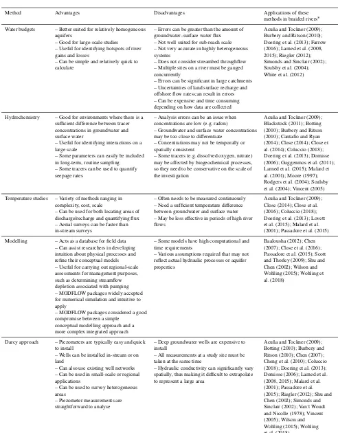
setting and scale of interaction to be measured (LaBaugh and Rosenberry, 2008). As a result of this review of studies in-vestigating groundwater–surface water exchange in braided rivers, a summary table has been developed (Table 1) that summarises the literature discussed in this paper and the ad-vantages and disadad-vantages of the various methods used in these studies.
The objectives of a study will influence which methods are most applicable. If only qualitative information about groundwater–surface water exchange is required, this could be obtained by methods such as mapping the locations of wet and dry reaches of a river, or identifying where there is mixing between groundwater and surface water based on chemical or heat tracers. Qualitative data will often assist in developing a conceptual understanding of the study site, which is a critical first step in data gathering. Alternatively, if quantitative data are needed, such as the rate of groundwa-ter seepage into a surface wagroundwa-ter body, this may be obtained by measuring Rn-222, analysing temperature signals, or by calculating the hydraulic gradient. Researchers have devel-oped flux quantification techniques for some of the meth-ods discussed in this paper (e.g. for temperature analysis see Gordon et al., 2012), but it is important to consider inputs required to calculate seepage through a streambed, such as streambed hydraulic conductivity (see Sect. 2.4). If direct water samples are needed, tools to consider could include groundwater wells or mini-piezometers. Water samples and flux rates can also be obtained using seepage meters, a com-mon method used for estimating groundwater–surface wa-ter inwa-teractions typically based on the design proposed by Lee (1977). However, it does not appear that these devices have been previously used in gravel-bed braided rivers. Seep-age meters have various limitations as discussed in previous studies (e.g. Kelly and Murdoch, 2003; Brodie et al., 2009; Cey et al., 1998), which indicate their application in braided rivers would be difficult and less effective than other meth-ods.
It is important to match the scale of the data required with the methods being used. This should include the consider-ation of both spatial and temporal scales. Remote sensing techniques such as airborne thermal infrared imaging and geophysics may prove useful to apply in braided river set-tings for gathering data on a large scale, as these methods have been used in braided rivers for geomorphological stud-ies (e.g. Huber and Huggenberger, 2016) and for investigat-ing groundwater–surface water exchange in other settinvestigat-ings (McLachlan et al., 2017). We discuss these approaches fur-ther in Sect. 4. It is important to recognise that it may be dif-ficult to accurately characterise smaller-scale groundwater– surface water interactions in highly heterogeneous braided river environments based on broad-scale methods. However, obtaining a broad snapshot of conditions or processes in a location may provide sufficient information to satisfy the study’s objectives. Also, using a combination of broad and point-scale techniques at a single study site may help
over-come the limitations of the individual techniques, particu-larly in heterogeneous environments (Kalbus et al., 2006).
Site-specific characteristics will largely determine the most appropriate methods to use relating to the geology, to-pography, hydrochemistry, hydrology and hydrogeology of the study site. Large braided rivers with high flows and deep channels may prove difficult to access directly. There is also a reasonable risk of the loss or damage of equipment installed in braided riverbeds due to floodwaters and sediment move-ment. These practical considerations underline the potential benefits of remote techniques to collect data in this type of river.
4 Key gaps and possibilities
This paper has highlighted that there are currently gaps in the knowledge of how groundwater and surface water inter-act in braided rivers. There is limited conceptual understand-ing of hyporheic flow processes, and how they impact river flow levels and water quality in braided rivers. The hyporheic zone has been highlighted as a significant area for ecological processes in rivers (Febria et al., 2011; Krause et al., 2011; Malard et al., 2001), but as Kalbus et al. (2006) note, it can be difficult to differentiate between hyporheic exchange and groundwater discharge. In addition, despite the contributions of the studies discussed here, the recharge rates to and from braided rivers continue to be an open question for water sci-entists and managers, as this has implications for both water quality and quantity. Measuring seepage rates is still difficult in many gravel-bed braided rivers, and often there is signif-icant uncertainty in the data collected. Lastly, there is still much scope for research on identifying historical patterns of dry and low-flow periods in braided river reaches. This is of-ten an area of significant concern for communities that are seeking answers on the correlations between dry or low-flow periods, and current and historical water use practices and climate.
Table 1.Advantages and disadvantages of various methodologies for measuring groundwater–surface water interactions in braided rivers.
Method Advantages Disadvantages Applications of these
methods in braided rivers∗ Water budgets – Better suited for relatively homogeneous – Errors can be greater than the amount of Acuña and Tockner (2009);
aquifers groundwater–surface water flux Burbery and Ritson (2010);
– Good for large-scale studies – Not well suited for sub-reach scale Doering et al. (2013); Farrow – Useful for identifying hotspots of river – Not very accurate in highly heterogeneous (2016); Larned et al. (2008,
gains and losses systems 2015); Riegler (2012);
– Can be simple and relatively quick to – Does not consider streambed throughflow Simonds and Sinclair (2002);
calculate – Multiple sites on a river must be gauged Soulsby et al. (2004);
concurrently White et al. (2012)
– Errors can be significant in large catchments – Uncertainties of land surface recharge and offshore flow rates can result in errors – Can be expensive and time consuming depending on how data are collected
Hydrochemistry – Good for environments where there is a – Analysis errors can be an issue when Acuña and Tockner (2009); sufficient difference between tracer concentrations are low (e.g. radon) Blackstock (2011); Botting concentrations in groundwater and – Groundwater and surface water concentrations (2010); Burbery and Ritson
surface water may be too close to differentiate (2010); Cantafio and Ryan
– Useful for identifying interactions on a – Concentrations may not be temporally or (2014); Close (2014); Close et
large scale spatially consistent al. (2014); Coluccio (2018);
– Some parameters can easily be included – Some tracers (e.g. dissolved oxygen, nitrate) Doering et al. (2013); Domisse in long-term, routine sampling may be affected by biogeochemical processes, (2006); Guggenmos et al. (2011); – Some tracers can be used to quantify so they need to be conservative on the scale of Larned et al. (2015); Malard et
seepage rates the investigation al. (2001); Moore (1997);
Rodgers et al. (2004); Soulsby et al. (2004); Vincent (2005) Temperature studies – Variety of methods ranging in – Often needs to be measured continuously Acuña and Tockner (2009);
complexity, cost, scale – Need a sufficient temperature difference Close (2014); Close et al. – Can be used for both locating areas of between groundwater and surface water (2016); Coluccio (2018); discharge/recharge and quantifying flux – May be less effective in periods of high river Doering et al. (2013); Lovett
– Aerial surveys can be faster than flows et al. (2015); Malard et al.
in-stream surveys (2001); Passadore et al. (2015)
Modelling – Acts as a database for field data – Some models have high computational and Baalousha (2012); Chen – Can assist researchers in developing time requirements (2007); Close et al. (2016); intuition about physical processes and – Various assumptions required that may not Passadore et al. (2015); Scott refine their conceptual models reflect actual hydraulic processes or aquifer and Thorley (2009); Shu and
– Useful for carrying out regional-scale properties Chen (2002); Wilson and
assessments for management purposes, Wohling (2015); Wohling et
such as determining streamflow al. (2018)
depletion associated with pumping – MODFLOW packages widely accepted for numerical simulation and intuitive to apply
– MODFLOW packages considered a good compromise between a simple
conceptual modelling approach and a more complex integrated approach
Darcy approach – Piezometers are typically easy and quick – Deep groundwater wells are expensive to Acuña and Tockner (2009);
to install install Botting (2010); Burbery and
– Wells can be installed in-stream or on – All measurements at a study site must be Ritson (2010); Chen (2007);
land taken at the same time Cheng et al. (2010); Coluccio
– Can also use existing well networks – Hydraulic conductivity can significantly vary (2018); Doering et al. (2013); – Can be used in small-scale or regional spatially, thus making it difficult to extrapolate Domisse (2006); Larned et al.
applications to represent a large area (2008, 2015); Malard et al.
– Can be used to survey heterogeneous (2001); Passadore et al.
areas (2015); Riegler (2012); Shu and
– Piezometer measurements are Chen (2002); Simonds and
straightforward to analyse Sinclair (2002); Van’t Woudt
and Nicolle (1978); Vincent (2005); Wilson and Wohling (2015); Wohling et al. (2018)
that can then be inferred to better conceptually understand groundwater–surface water exchange. There is also scope for more remote collection of data, and Carbonneau and Pié-gay (2012) review a range of techniques for use in rivers, while Marcus (2012) provides an overview of remote sens-ing specifically in gravel-bed rivers. There is a significant amount of freely available satellite data (e.g. via the Sentinel satellites, https://sentinel.esa.int/web/sentinel/home, last ac-cess: 22 October 2019) that may be useful in braided river studies. Unmanned aerial vehicles have become more afford-able and advanced in recent years, allowing for remote col-lection of a range of data on rivers such as thermal infrared, multispectral and hyperspectral imaging, and photogramme-try (Pai et al., 2017).
Artificial dye, chemical (e.g. salt) or bacterial tracers are often useful for shedding light on processes such as ground-water velocity and flow paths or hyporheic zone flow (Flury and Wai, 2003). They have been used in other types of rivers to investigate groundwater–surface water exchange (e.g. Bin-ley et al., 2013; Ferreira et al., 2018; Stoner et al., 2013; Knöll and Scheytt, 2018; González-Pinzón et al., 2015). Sev-eral studies have used rhodamine dye in a New Zealand well array installed in an alluvial aquifer deposited by braided rivers to estimate hydraulic properties and examine ground-water flow paths (e.g. Close et al., 2002; Dann et al., 2008; Sarris et al., 2018). For artificial tracer tests to be time and cost effective, some prior knowledge of water flow paths and velocities is necessary (Close et al., 2002).
There is scope to use other temperature methods than those described in Sect. 2.3, such as fibre-optic distributed temper-ature sensing (FODTS) (Busato et al., 2019; Klinkenberg, 2015; Lovett et al., 2015; Meijer, 2015; Rosenberry et al., 2016; Mwakanyamale et al., 2012) or active heat pulse meth-ods (see Briggs et al., 2016; Banks et al., 2018). Collection of temperature profiles was briefly mentioned in Sect. 2.3 in the study conducted by Coluccio (2018), which used 1-D temperature profiles. However, there are several ways tem-perature profiles can be collected (1-D, 2-D, 3-D), as well as a range of analysis methods that can be used, as demon-strated in several previous studies in non-braided river set-tings (Briggs et al., 2014; Gordon et al., 2013; Naranjo and Turcotte, 2015; Rosenberry et al., 2016). There is also con-siderable scope for applying thermal infrared (TIR) imaging in braided rivers. Handcock et al. (2012) provide a compre-hensive review of the use of TIR imaging in rivers. Using TIR imaging to highlight temperature differences in a braided streambed may be particularly useful for qualitatively iden-tifying locations of groundwater inflow to rivers. TIR data can be collected remotely (by UAV, helicopter or fixed-wing plane), on the ground or by satellite, and there are impor-tant considerations with each category (e.g. cost, scale of data collected). TIR imaging has been used in several river envi-ronments to identify groundwater–surface water interactions (Culbertson et al., 2013; Eschbach et al., 2017; Hare et al., 2015; Liu et al., 2016; Lovett et al., 2015; Rautio et al., 2018)
but does not appear to have been applied in braided rivers to any great extent for this purpose.
There have been many advances in geophysical tech-niques in recent years, and these methods do not appear to have been applied in braided river settings for investi-gations of groundwater–surface water exchange. McLachlan et al. (2017) provide a thorough recent review of geophysi-cal methods for characterising the groundwater–surface wa-ter inwa-terface, such as electrical resistivity tomography (ERT), ground penetrating radar (GPR), seismic methods, and for-ward and inverse geophysical modelling. These methods al-low for river systems to be characterised where factors such as geological, hydrological and biogeochemical heterogene-ity make it difficult to make direct measurements (McLach-lan et al., 2017). Geophysical methods may be particularly useful for characterising subsurface structures in braided rivers, which are poorly understood. A recent study by Busato et al. (2019) demonstrates the use of ERT and FODTS in a rocky stream with poorly sorted substrate, the results of which may provide useful insight for braided river applica-tions. Examples of studies in other types of river environ-ments that used geophysics to characterise the groundwater– surface water interface include Singha et al. (2008), Binley et al. (2013) and Steelman et al. (2017). Geophysical data can also be collected remotely in airborne electromagnetic surveys such as in Harrington et al. (2014). As McLachlan et al. (2017) note, geophysical techniques should be used to complement data collected by other hydrological and biogeo-chemical methods.
5 Summary
Braided rivers are unique and dynamic river environments that perform important ecological, cultural, recreational and freshwater resource functions. A critical aspect of their ef-fective management is understanding groundwater and sur-face water interactions in these rivers and their associated aquifers. This article provides an overview of characteristics specific to braided rivers, which include multiple meandering channels that often shift, temporary and semi-permanent bars and islands, wide active riverbed areas, heterogeneous and (typically) mixed sand and gravel streambeds, and a signif-icant portion of river flow that occurs within the streambed. We present a map showing the regions where braided rivers are mainly found at the global scale: Alaska, Canada, the Japanese and European Alps, the Himalayas, Russia, and New Zealand. To the authors’ knowledge, this is the first map of its kind. Our review of prior studies of surface water-groundwater interactions in braided rivers showed that most studies have been recent (in the past 10–20 years), and they have investigated a range of questions including calculating seepage rates to and from braided rivers, estimating time lags between rivers and groundwater, and looking at the implica-tions of groundwater–surface water exchange on ecological processes. We also investigated the effectiveness of the var-ious methods used in the studies identified in this review in terms of achieving the studies’ objectives and their applica-bility in braided rivers. A table has been produced summaris-ing these findsummaris-ings and shows that there is a variety of avail-able methods ranging in cost and scale.
Lastly, this article explored the various considerations one may make when choosing appropriate techniques for in-vestigating groundwater–surface water exchange in braided rivers. The use of multiple methods at varying spatial scales at a single study site may help overcome the uncertainties associated with data gathered in heterogeneous, dynamic braided river environments. Given the challenges of work-ing directly in braided rivers, there is considerable scope for the increased use of remote sensing techniques and geo-physics. There is also scope for new approaches to modelling braided rivers using integrated techniques that incorporate the often-complex river bed terrain and geomorphology of braided rivers explicitly. There is presently limited under-standing of how hyporheic zone processes operate and im-pact braided rivers, recharge rates to and from braided rivers, and historic drying and low-flow trends in braided rivers, and thus future research is needed in these areas. While only some of the methods discussed here allow for quantification of groundwater–surface water flux, many of these techniques can improve our conceptual understanding of these systems and processes.
Data availability. No data sets were used in this article.
Author contributions. The project was instigated by LKM. KC car-ried out the literature review that formed the content of this paper. KC and LKM wrote the paper.
Competing interests. The authors declare that they have no conflict of interest.
Acknowledgements. The authors would like to thank
Zeb Etheridge, Philippa Aitchison-Earl, Graeme Horrell, Fouad Alkhaier and Scott Wilson for comments on this manuscript. The authors also thank the four anonymous reviewers for their constructive feedback.
Financial support. This research has been supported by the Can-terbury Regional Council and the Waterways Centre for Freshwater Management.
Review statement. This paper was edited by Patricia Saco and re-viewed by four anonymous referees.
References
Acuña, V. and Tockner, K.: Surface-subsurface water exchange rates along alluvial river reaches control the thermal patterns in an Alpine river network, Freshwater Biol., 54 306–320, https://doi.org/10.1111/j.1365-2427.2008.02109.x, 2009. Alexeevsky, N. I., Chalov, R. S., Berkovich, K. M., and Chalov, S.
R.: Channel changes in largest Russian rivers: Natural and an-thropogenic effects, Int. J. River Basin Manage., 11, 175–191, https://doi.org/10.1080/15715124.2013.814660, 2013.
Al-Hazaimay, S., Huisman, J. A., Zimmermann, E., and Vereecken, H.: Using electrical anisotropy for structural characterization of sediments: An experimental validation study, Near Surf. Geo-phys., 14, 357–369, https://doi.org/10.3997/1873-0604.2016026, 2016.
Andersen, M. S.: Heat as a Ground Water Tracer, Ground Water, 43, 951–968, https://doi.org/10.1111/j.1745-6584.2005.00052.x, 2005.
Ashmore, P.: Laboratory modelling of gravel braided stream morphology, Earth Surf. Proc. Land., 7, 201–225, https://doi.org/10.1002/esp.3290070301, 1982.
Ashmore, P.: Anabranch confluence kinetics and sedimentation pro-cesses in gravel-braided streams, in: Braided Rivers, edited by: Best, J. L. and Bristow, C. S., Geological Society Special Pub-lication No. 75, The Geological Society, Bath, UK, 129–146, 1993.
Baalousha, H. M.: Characterisation of groundwater–surface water interaction using field measurements and numeri-cal modelling: A case study from the Ruataniwha Basin, Hawke’s Bay, New Zealand, Appl. Water Sci., 2, 109–118, https://doi.org/10.1007/s13201-012-0028-3, 2012.
De-velopment Using Python and FloPy, Groundwater, 54, 733–739, https://doi.org/10.1111/gwat.12413, 2016.
Bandini, F., Butts, M., Vammen Jacobsen, T., and Bauer-Gottwein, P.: Water level observations from unmanned aerial vehicles for improving estimates of surface water–groundwater interaction, Hydrol. Process., 31, 4371–4383, 10.1002/hyp.11366, 2017. Banks, E. W., Shanafield, M. A., Noorduijn, S., McCallum, J.,
Lewandowski, J., and Batelaan, O.: Active heat pulse sensing of 3-D-flow fields in streambeds, Hydrol. Earth Syst. Sci., 22, 1917–1929, https://doi.org/10.5194/hess-22-1917-2018, 2018. Barlow, P. M. and Harbaugh, A. W.: USGS Directions in
MODFLOW Development, Ground Water, 44, 771–774, https://doi.org/10.1111/j.1745-6584.2006.00260.x, 2006. Bernini, A., Caleffi, V., and Valiani, A.: Numerical modelling of
alternate bars in shallow channels, in: Braided Rivers, edited by: Sambrook Smith, G. H., Best, J. L., Bristow, C. S., and Petts, G. E., Blackwell Publishing, Malden, MA, USA, 153–175, 2006. Binley, A., Ullah, S., Heathwaite, A. L., Heppell, C., Byrne,
P., Lansdown, K., Trimmer, M., and Zhang, H.: Revealing the spatial variability of water fluxes at the groundwater-surface water interface, Water Resour. Res., 49, 3978–3992, https://doi.org/10.1002/wrcr.20214, 2013.
Blackstock, J.: Isotope study of moisture sources, recharge areas, and groundwater flow paths within the Christchurch Groundwa-ter System, MasGroundwa-ter of Science in Geology, Geology, University of Canterbury, Christchurch, New Zealand, available at: https: //ir.canterbury.ac.nz/handle/10092/7042 (last access: 22 Octo-ber 2019), 2011.
Boano, F., Harvey, J. W., Marion, A., Packman, A. I., Rev-elli, R., Ridolfi, L., and Wörman, A.: Hyporheic flow and transport processes: Mechanisms, models, and bio-geochemical implications, Rev. Geophys., 52, 603–679, https://doi.org/10.1002/2012RG000417, 2014.
Botting, J.: Groundwater flow patterns and origin on the North Bank of the Wairau River, Marlborough, New Zealand, Mas-ter of Science in Engineering Geology, Geology, University of Canterbury, Christchurch, New Zealand, available at: https: //ir.canterbury.ac.nz/handle/10092/5519 (last access: 22 Octo-ber 2019), 2010.
Briggs, M. A., Lautz, L. K., Buckley, S. F., and Lane, J. W.: Prac-tical limitations on the use of diurnal temperature signals to quantify groundwater upwelling, J. Hydrol., 519, 1739–1751, https://doi.org/10.1016/j.jhydrol.2014.09.030, 2014.
Briggs, M. A., Buckley, S. F., Bagtzoglou, A. C., Werkema, D. D., and Lane, J. W.: Actively heated high-resolution fiber-optic-distributed temperature sensing to quantify streambed flow dy-namics in zones of strong groundwater upwelling, Water Resour. Res., 52, 5179–5194, https://doi.org/10.1002/2015WR018219, 2016.
Brodie, R. S., Sundaram, B., Tottenham, R., Hostetler, S., and Rans-ley, T.: An overview of tools for assessing groundwater-surface water connectivity, Bureau of Rural Sciences, Canberra, Aus-tralia, 2007.
Brodie, R. S., Baskaran, S., Ransley, T., and Spring, J.: Seepage meter: Progressing a simple method of di-rectly measuring water flow between surface water and groundwater systems, Aust. J. Earth Sci., 56, 3–11, https://doi.org/10.1080/08120090802541879, 2009.
Brown, L. J.: Canterbury, in: Groundwaters of New Zealand, edited by: Rosen, M. R. and White, P. A., New Zealand Hydrological Society Inc, Wellington, 441–459, 2001.
Brunner, P., Cook, P. G., and Simmons, C. T.: Hydro-geologic controls on disconnection between surface wa-ter and groundwawa-ter, Wawa-ter Resour. Manage., 45, W01422, https://doi.org/10.1029/2008WR006953, 2009.
Brunner, P., Simmons, C. T., Cook, P. G., and Therrien, R.: Modeling Surface Water–Groundwater Interaction with MOD-FLOW: Some Considerations, Ground Water, 48, 174–180, https://doi.org/10.1111/j.1745-6584.2009.00644.x, 2010. Brunner, P., Therrien, R., Renard, P., Simmons, C. T., and
Franssen, H.-J. H.: Advances in understanding river-groundwater interactions, Rev. Geophys., 55, 818–854, https://doi.org/10.1002/2017RG000556, 2017.
Burbery, L., and Ritson, J.: Integrated study of surface water and shallow groundwater resources of the Orari catchment, R10/36, Environment Canterbury, Christchurch, New Zealand, available at: http://docs.niwa.co.nz/library/public/ECtrR10-36. pdf (last access: 15 March 2019), 2010.
Burnett, W. C., Kim, G., and Lane-Smith, D.: A contin-uous monitor for assessment of 222Rn in the coastal ocean, J. Radioanal. Nucl. Chem., 249, 167–172, https://doi.org/10.1023/A:1013217821419, 2001.
Busato, L., Boaga, J., Perri, M. T., Majone, B., Bellin, A., and Cassiani, G.: Hydrogeophysical characterization and monitor-ing of the hyporheic and riparian zones: The Vermigliana Creek case study, Sci. Total Environ., 648, 1105–1120, https://doi.org/10.1016/j.scitotenv.2018.08.179, 2019.
Butts, M., Feng, K., Klinting, A., Stewart, K., Nath, A., Man-ning, P., Hazlett, T., Jacobsen, T., and Larsen, J.: Real-time sur-face water-ground water modelling of the Big Cypress Basin, Florida, DHI Water & Environment, Horsholm, Denmark, avail-able at: http://feflow.info/fileadmin/FEFLOW/content_tagung/ TagungsCD/papers/31.pdf, last access: 11 April 2019.
Cantafio, L. J. and Ryan, M. C.: Quantifying baseflow and water-quality impacts from a gravel-dominated alluvial aquifer in an urban reach of a large Canadian river, Hydrogeol. J., 22, 957– 970, https://doi.org/10.1007/s10040-013-1088-7, 2014. Carbonneau, P. E. and Piegay, H.: Fluvial Remote Sensing for
Sci-ence and Management, 1st Edn., Advancing River Restoration and Management Series, John Wiley & Sons, West Sussex, UK, 2012.
Cardenas, M. B.: Hyporheic zone hydrologic science: A historical account of its emergence and a prospectus, Water Resour. Res., 51, 3601–3616, https://doi.org/10.1002/2015WR017028, 2015. Caruso, B. S.: Project river recovery: Restoration of braided
gravel-bed river habitat in New Zealand’s high country, Environ. Man-age., 37, 840–861, https://doi.org/10.1007/s00267-005-3103-9, 2006.
Cey, E. E., Rudolph, D. L., Parkin, G. W., and Aravena, R.: Quantifying groundwater discharge to a small perennial stream in southern Ontario, Canada, J. Hydrol., 210, 21–37, https://doi.org/10.1016/s0022-1694(98)00172-3, 1998.