Spatial and temporal variation in river corridor exchange across a 5th order mountain stream network

https://doi.org/10.5194/hess-23-5199-2019 © Author(s) 2019. This work is distributed under the Creative Commons Attribution 4.0 License.

Spatial and temporal variation in river corridor exchange across a

5th-order mountain stream network

Adam S. Ward1, Steven M. Wondzell2, Noah M. Schmadel1,3, Skuyler Herzog1, Jay P. Zarnetske4, Viktor Baranov5,6, Phillip J. Blaen7,8,9, Nicolai Brekenfeld7, Rosalie Chu10, Romain Derelle11, Jennifer Drummond7,12,

Jan H. Fleckenstein13,14, Vanessa Garayburu-Caruso15, Emily Graham15, David Hannah7, Ciaran J. Harman16, Jase Hixson1, Julia L. A. Knapp17,18, Stefan Krause7, Marie J. Kurz13,19, Jörg Lewandowski20,21, Angang Li22, Eugènia Martí12, Melinda Miller1, Alexander M. Milner7, Kerry Neil1, Luisa Orsini11, Aaron I. Packman22, Stephen Plont4,23, Lupita Renteria24, Kevin Roche25, Todd Royer1, Catalina Segura26, James Stegen15, Jason Toyoda10, Jacqueline Wells24, and Nathan I. Wisnoski27

1_{O’Neill School of Public and Environmental Affairs, Indiana University, Bloomington, Indiana, USA} 2_{USDA Forest Service, Pacific Northwest Research Station, Corvallis, Oregon, USA}

3_{USGS Earth Surface Processes Division, U.S. Geological Survey, Reston, Virginia, USA}

4_{Department of Earth and Environmental Sciences, Michigan State University, East Lansing, Michigan, USA} 5_{LMU Munich Biocenter, Department of Biology II, Großhaderner Str. 2, 82152 Planegg-Martinsried, Germany} 6_{Department of River Ecology and Conservation, Senckenberg Research Institute and Natural History Museum,} 63571 Gelnhausen, Germany

7_{School of Geography, Earth & Environmental Sciences, University of Birmingham, Edgbaston, Birmingham, B15 2TT, UK} 8_{Birmingham Institute of Forest Research (BIFoR), University of Birmingham, Edgbaston, Birmingham, B15 2TT, UK} 9_{Yorkshire Water, Halifax Road, Bradford, BD6 2SZ, UK}

10_{Environmental Molecular Sciences Laboratory, Pacific Northwest National Laboratory, Richland, Washington, USA} 11_{Environmental Genomics Group, School of Biosciences, the University of Birmingham, Birmingham, B15 2TT, UK} 12_{Integrative Freshwater Ecology Group, Centre for Advanced Studies of Blanes (CEAB-CSIC), Blanes, Spain}

13_{Dept. of Hydrogeology, Helmholtz Center for Environmental Research – UFZ, Permoserstraße 15, 04318 Leipzig, Germany} 14_{Bayreuth Center of Ecology and Environmental Research, University of Bayreuth, 95440 Bayreuth, Germany}

15_{Earth and Biological Sciences Division, Pacific Northwest National Laboratory, Richland, Washington, USA} 16_{Department of Environmental Health and Engineering, Johns Hopkins University, Baltimore, Maryland, USA} 17_{Department of Environmental Systems Science, ETH Zürich, Zurich, Switzerland}

18_{Center for Applied Geoscience, University of Tübingen, Tübingen, Germany}

19_{The Academy of Natural Sciences of Drexel University, Philadelphia, Pennsylvania, USA} 20_{Leibniz Institute of Freshwater Ecology and Inland Fisheries, Department of Ecohydrology,} Müggelseedamm 310, 12587 Berlin, Germany

21_{Humboldt University Berlin, Geography Department, Rudower Chaussee 16, 12489 Berlin, Germany} 22_{Department of Civil and Environmental Engineering, Northwestern University, Evanston, Illinois, USA}

23_{Department of Biological Sciences, Virginia Polytechnic Institute and State University, Blacksburg, Virginia, USA} 24_{Pacific Northwest National Laboratory, Richland, Washington, USA}

25_{Department of Civil & Environmental Engineering & Earth Sciences, University of Notre Dame, Notre Dame, Indiana, USA} 26_{Forest Engineering, Resources, and Management, Oregon State University Corvallis, Oregon, USA}

27_{Department of Biology, Indiana University, Bloomington, Indiana, USA} Correspondence:Adam S. Ward ([email protected])

Received: 8 March 2019 – Discussion started: 23 April 2019

Abstract.Although most field and modeling studies of river corridor exchange have been conducted at scales ranging from tens to hundreds of meters, results of these studies are used to predict their ecological and hydrological influences at the scale of river networks. Further complicating predic-tion, exchanges are expected to vary with hydrologic forcing and the local geomorphic setting. While we desire predic-tive power, we lack a complete spatiotemporal relationship relating discharge to the variation in geologic setting and hy-drologic forcing that is expected across a river basin. Indeed, the conceptual model of Wondzell (2011) predicts systematic variation in river corridor exchange as a function of (1) vari-ation in baseflow over time at a fixed locvari-ation, (2) varivari-ation in discharge with location in the river network, and (3) local geomorphic setting. To test this conceptual model we con-ducted more than 60 solute tracer studies including a synop-tic campaign in the 5th-order river network of the H. J. An-drews Experimental Forest (Oregon, USA) and replicate-in-time experiments in four watersheds. We interpret the data using a series of metrics describing river corridor exchange and solute transport, testing for consistent direction and mag-nitude of relationships relating these metrics to discharge and local geomorphic setting. We confirmed systematic de-crease in river corridor exchange space through the river net-works, from headwaters to the larger main stem. However, we did not find systematic variation with changes in dis-charge through time or with local geomorphic setting. While interpretation of our results is complicated by problems with the analytical methods, the results are sufficiently robust for us to conclude that space-for-time and time-for-space substi-tutions are not appropriate in our study system. Finally, we suggest two strategies that will improve the interpretability of tracer test results and help the hyporheic community develop robust datasets that will enable comparisons across multiple sites and/or discharge conditions.

1 Introduction

Ecological functions and processes in the river corridor are influenced by the exchange of water, solutes, and energy be-tween the surface stream and its catchment and thus regulate downstream water quality (e.g., Brunke and Gonser, 1997; Krause et al., 2011; Wondzell and Gooseff, 2014; Ward, 2015). These exchange fluxes are collectively termed river corridor exchange and integrate the stream, hyporheic zone, and riparian zone along the river network (Harvey and Goos-eff, 2015). Several recent studies have extended feature- and reach-scale findings to predict ecological functions of river corridors at basin scales relevant to resource management (e.g., Gomez-Velez and Harvey, 2014; Kiel and Cardenas, 2014; Gomez-Velez et al., 2015; Bertuzzo et al., 2017; Hel-ton et al., 2018). These approaches require a scaling

rela-tionship to predict river corridor exchange across space and through time. Discharge is a logical scaling factor and has been studied as a control on river corridor exchange in both space (i.e., along a network) and time (i.e., under differ-ent hydrologic conditions at a fixed location). However, dis-charge integrates forcing at different scales and may not lead to consistent predictions of river corridor exchange (Ward and Packman, 2019). For example, increases in discharge have been found to cause increases, decreases, or no change in river corridor exchange (Morrice et al., 1997; Butturini and Sabater, 1999; Hart et al., 1999; Jin and Ward, 2005; Wondzell, 2006, 2011; Zarnetske et al., 2007; Schmid, 2008; Karwan and Saiers, 2009; Schmid et al., 2010; Fabian et al., 2011; Ward et al., 2013a). Clearly, to use discharge as a scal-ing factor to predict river corridor exchange, a more com-plete description of the exchange–discharge relationship is required.

exchange with increased discharge due to compression of hyporheic flow paths by toward-stream hydraulic gradients (e.g., Hakenkamp et al., 1993; Hynes, 1983; Palmer, 1993; Vervier et al., 1992; White et al., 1993).

The second primary control on river corridor exchange is the geomorphic setting, including differences attributable to tectonics (e.g., Valett et al., 1996; Payn et al., 2009). Over geologic timescales the geomorphic setting has co-evolved with hydrologic forcing. For example, as drainage area and discharge accumulate through mountain stream net-works, we expect predictable spatial patterns including lower slopes, smaller grain size, larger channel width-to-depth ra-tios, and increased valley bottom widths (e.g., Leopold and Maddock, 1953; Wohl and Merritt, 2005, 2008; Brardinoni and Hassan, 2007). The evolution of geologic setting oc-curs over an extremely long timescale, allowing the common simplification of assuming geologic setting as static in hy-porheic studies. As a result of this assumption, researchers commonly conduct experiments across a spatial gradient to describe patterns in river corridor exchange (Payn et al., 2009; Covino et al., 2011; Mallard et al., 2014). This ap-proach provides a fixed-in-time, varied-in-space river cor-ridor exchange–discharge relationship that describes a net-work under a fixed hydrologic condition, most commonly baseflow. Wondzell (1994) suggested that exchange should decrease with increasing watershed size based on first prin-ciples. For example, the potential maximum exchange is lim-ited by the streambed area, indicating that the ratio of wetted perimeter to discharge (Q) should be correlated to the max-imum possible exchange per unit length of stream channel. AsQincreases more rapidly than wetted perimeter as wa-tersheds increase in size, the amount of exchange should be expected to decrease. In fact, most studies have identified a decreasing role of river corridor exchange as river basins increase in size, attributable to less exchange flux relative to stream flow (Stewart et al., 2011; Mallard et al., 2014; Gomez-Velez and Harvey, 2014; Kiel and Cardenas, 2014; Gomez-Velez et al., 2015; Ward et al., 2018a).

To explain spatiotemporal patterns in river corridor ex-change from headwaters to large rivers, Wondzell (2011) developed a conceptual framework describing the relative importance of river corridor exchange to reach-scale trans-port (i.e., hyporheic exchange flow normalized by river discharge, QHEF/Q), spanning three primary dimensions. First, QHEF/Q would be largest under the lowest steady-state discharge conditions, where subsurface flow may re-flect a larger proportion of total down-valley flow. Second,

QHEF/Q would be largest in the headwaters and decrease moving toward larger river segments as described above. Lastly, Wondzell (2011) characterized the local geomorphic setting at an individual study site as “hyporheic potential,” combining valley slope and hydraulic conductivity to reflect local controls on exchange at the reach scale that might vary locally within the systematic spatial and temporal dimen-sions. Larger hyporheic potential was associated with larger

QHEF/Q. Subsequently, Harvey et al. (2018) suggested that hydrologic connectivity (i.e., QHEF/Q) is a primary water quality regulator. Ward et al. (2018a) further extended this concept to account for changes in valley bottom width and depth of colluvium, describing the down-valley capacity of the valley bottom to transmit water estimated via Darcy’s law. Unlike the first two dimensions, hyporheic potential may not have a predictable trend as one moves down a river con-tinuum because decreasing slopes and hydraulic conductivi-ties may be offset by larger hyporheic cross sections.

Efforts to predict river corridor exchange and associated ecosystem processes as a function of geomorphic setting and hydrologic forcing have been implemented in large-scale re-motely sensed test cases. However, this method still lacks field validation across varying discharge and across a range of stream types with varying morphologic features. For ex-ample, Gomez-Velez and Harvey (2014) and Gomez-Velez et al. (2015) used the Networks with EXchange and Subsur-face Storage (NEXSS) model to describe spatial patterns in exchange in low-gradient alluvial river networks. NEXSS is based on steady-state discharge and bed sediment grain size as a proxy for local morphologic control. While this model-ing approach has demonstrated the importance of river corri-dor exchange in large river basins, it is built on scaling rela-tionships derived from idealized mechanistic and conceptual models that may not be representative of headwater streams. Further, the model results have yet to be confirmed in field trials.

To our knowledge, only the field study of Payn et al. (2009) explicitly considered both spatial and temporal dimensions of the exchange–discharge relationship. The re-sults of that study were broadly consistent with the concep-tual model of Wondzell (2011). However, we now understand that fixed reach lengths cause systematic decreases in the “window of detection” (the timescale of exchange flow paths that are measurable with tracer studies; Harvey et al., 1996; Wagner and Harvey, 1997; Harvey and Wagner, 2000). The systematic decrease in window of detection with increasing discharge along the study stream would have interacted with the fixed reach lengths, likely leading to the underestimation ofQHEFat high discharges. As a result, it is difficult to sep-arate the observed process from limitations of the measure-ment instrumeasure-ment (see discussion of the data of Payn et al. in Ward et al., 2013b, and similar studies by Schmadel et al., 2016a).

date, the conceptual model of Wondzell (2011) lacks valida-tion across large river basins studied with a systematic field approach. Given the variability of reach-scale river corridor exchange trends documented in the literature (see summary in Ward and Packman, 2019), it is critical to test the con-ceptual model of Wondzell (2011) with field data that cover much more of the space-time parameter space.

In this study, we seek to characterize river corridor ex-change in a mountain stream network as a function of (1) variation in baseflow at a fixed location through sea-sonal recession, (2) variation in discharge as a function of drainage area during a fixed baseflow condition, and (3) lo-cal geomorphic setting (quantified here as hyporheic poten-tial). This study will directly test the conceptual model posed by Wondzell (2011) for mountain stream networks. If the conceptual relationships can be confirmed, this would en-able transferability of findings from feature- and reach-scale studies to entire networks of high-gradient mountain streams, paralleling recent advances in low-gradient river networks (e.g., Gomez-Velez and Harvey, 2014; Kiel and Cardenas, 2014; Gomez-Velez et al., 2015). Further, confirmation of the conceptual model would provide a simple scaling rela-tionship for time-variable discharge, which has not been pos-sible to date. In this study, we conducted a series of solute tracer studies to construct temporal exchange–discharge re-lationships (i.e., a fixed study reach with observations span-ning a range in discharge) and spatial exchange–discharge relationships (i.e., a synoptic campaign to measure exchange at many locations under summer baseflow discharge) for a 5th-order mountain river network, together with physical ob-servations (including hydraulic conductivity, drainage area, slope, valley bottom width, sinuosity) to also characterize hyporheic potential. We interpret the data using a series of metrics describing river corridor exchange and their relation-ships to discharge.

2 Methods

2.1 Field site and solute tracer experiments 2.1.1 Site description

The H. J. Andrews Experimental Forest (HJA) is a 5th-order basin draining about 6400 ha in the western Cascade Moun-tains, Oregon, USA, with elevations ranging from about 410 to 1630 m a.m.s.l. The basin is heavily forested and includes stands of old growth Douglas fir trees as well as smaller ar-eas that have been logged to study the effects of forest man-agement practices. Additional details about the climate, mor-phology, geology, and ecology of the site are well described by others (Dyrness, 1969; Swanson and James, 1975; Swan-son and Jones, 2002; JefferSwan-son et al., 2004; Cashman et al., 2009; Deligne et al., 2017). The synoptic sampling spanned the entire HJA basin to characterize basin-scale valley

bot-tom conditions, while additional, more detailed sampling oc-curred in three distinct landform types.

Headwater sites in the HJA generally fall into one of three landform types associated with underlying geology and geomorphic processes (Table 1). We selected four 2nd-order basins to establish fixed stream reaches for replication through the summer baseflow recession period, one in each landform type plus one replicate. The first landform type occurs in the lower elevations of the HJA where geology is dominated by upper Oligocene–lower Miocene basaltic flows. These volcanoclastic rocks were weakened by hy-drothermal alteration from subsequent volcanic activity, en-abling rapid downcutting and formation of a highly dissected landscape. Hillslopes are steep; valleys are v-shaped and tend to be narrow with steep longitudinal gradients. Valley bot-tom colluvium is typically shallow but variable, being em-placed by hillslope mass wasting and debris flows. Exposed bedrock is visible in many locations, while deeper deposits form behind individual large logs or larger log jams. We selected the well-studied Watersheds 1 and 3 (WS01 and WS03) for two of our fixed reaches (Fig. 1). Briefly, WS01 and WS03 valley bottoms reflect different time periods in this landform. In 1996, WS03 was scoured to bedrock along hun-dreds of meters of the valley bottom (Johnson, 2004). Since that time no debris flows have been recorded, resulting in a study reach nearly free of colluvium in the upper half of the study reach. WS01 is a paired catchment to WS03, reason-ably representing a pre-scour and less-constrained compari-son to WS03. WS01 has a wood-forced step-pool morphol-ogy (Montgomery and Buffington, 1997, 1998) over most of its main stem length, representative of many steep moun-tain streams. River corridor exchange in the two catchments has been broadly studied using a paired catchment approach (e.g., Wondzell, 2006; Voltz et al., 2013; Ward et al., 2017b). Deep-seated earth flows provide a second contrasting land-form type in the HJA. These are emplaced on the upper Oligocene–lower Miocene basaltic flows and are character-ized by a poorly developed channel network (many parallel channels), a general lack of lateral contributing area to the river corridor, little lateral constraint, and extensive colluvial deposits with no bedrock exposure. Based on visual inspec-tion, channels on these earthflows are actively meandering, braiding, and downcutting. Characteristic geomorphic fea-tures include meander bends and cutbanks (visually simi-lar to lower-gradient alluvial systems of the region) in addi-tion to step-pool features. We selected an unnamed 2nd-order reach on a large earth flow adjacent to WS03 for this study (Fig. 1).

con-Table 1.Summary of key characteristics of the fixed-reach sites. See detailed descriptions for further information (Dyrness, 1969; Swanson and James, 1975; Swanson and Jones, 2002; Jefferson et al., 2004; Cashman et al., 2009; Deligne et al., 2017).

Site Important hydrologic controls Important geologic controls

WS01 – Highly dissected landscape

– Focused lateral inflows

– Diurnal discharge fluctuations due to evapotranspira-tion

– Colluvium deposited by debris flows from hillslopes forms extensive deposits in the valley bottom

– V-shaped, rapidly downcutting valley

WS03 – Highly dissected landscape

– Focused lateral inflows

– Diurnal discharge fluctuations due to evapotranspira-tion

– Scoured to bedrock in 1996 leaving only small colluvial deposits

– Highly constrained, low colluvium analogue to WS01 – V-shaped, rapidly downcutting valley

Unnamed cr. – Surficial aquifer on earthflow connects several parallel

channels

– Minimal lateral tributary area

– Deep-seated earthflow

– No defined valley; parallel stream channels down hills-lope

Cold Cr. – Extensive aquifer provides high discharge, cold

base-flow year-round – Diffuse lateral inflows

– Compressed glacial tills – U-shaped valley (glacial cirque) – Uniform lateral tributary area

Figure 1.Synoptic study sites and lidar-derived stream network for the H. J. Andrews Experimental Forest. Reprinted with permission from Ward et al. (2019).

trast to the highly dissected landforms in WS01 and WS03). Bedrock is rarely visible along the study site. We selected a 2nd-order reach of Cold Creek to represent this landform (Fig. 1).

2.1.2 Synoptic study

We conducted a synoptic study at 46 sites within the HJA during late summer baseflow conditions (Fig. 1) that in-cluded solute tracer experiments. Site selection was strati-fied by stream order so that more headwater sites were

de-scribed in detail by Ward et al. (2019), but we provide an overview below.

At each site we measured mean stream width and depth, valley width, and collected GPS coordinates. Subsequently, a modified version of TopoToolbox 2.0 (Schwanghart and Kuhn, 2010; Schwanghart and Scherler, 2014) and a 1 m lidar-derived, digital elevation model (DEM) was used to extract upslope accumulated area (UAA, ha), valley slope (Sval, m m−1), and a stream centerline that was used to cal-culate sinuosity (sinuosity, m m−1). Our methods were iden-tical to those previously used in the basin (Corson-Rikert et al., 2016; Schmadel et al., 2017; Ward et al., 2018a, c).

At each synoptic site, we drove a Solinst 615N well point into the streambed so that the top of the 0.15 m screened interval was 50 cm below the streambed. After developing the well with a peristaltic pump, we conducted three to six replicate falling head tests, measuring head change through time using a down-well Van Essen Micro-Diver logging at 0.5 s intervals. Falling head tests were interpreted using the Hvorslev (1951) method:

K=

r2lnLe

R

2LeT0

, (1)

whereKis hydraulic conductivity (m s−1),ris the radius of the well casing (0.025 m),R is the radius of the well screen (0.005 m),Leis the screened length of the well (m), andT0is the time for the head to fall to about 37 % of its original value (i.e., thee-folding time, s). We took the geometric mean of the replicate tests as the representative value of K at each site.

We calculated the capacity of the subsurface to convey wa-ter down the valley bottom (Qsub,cap, sometimes termed “un-derflow”, m3s−1)as

Qsub,cap=bvalleyhvalleyKSval (2)

following Ward et al. (2018a), where bvalley is the valley width,hvalleyis the valley colluvium depth (m, estimated as 50 % of the wetted channel width). This estimate is consis-tent with depths used in past studies (Gooseff et al., 2006; Ward et al., 2012, 2018a, c; Crook et al., 2008; Schmadel et al., 2017) and geophysical transects in the 4th- and 5th-order reaches of Lookout Creek (Steven M. Wondzell, unpublished data). We calculated hyporheic potential (HYPPOT, m s−1) after Wondzell (2011), a similar metric that does not account for valley width, depth, or porosity, as

HYPPOT=SvalK. (3)

We also calculated stream power (, W m−2) at each tracer release location as

=ρgQS, (4)

whereρ is the density of water (kg m−3),g is the gravita-tional constant (9.81 m s−2), Qis the average discharge in

the study segment (m3s−1), andSis the DEM-derived slope along the stream channel in the study segment (m m−1_).

Finally, at each site, we established a stream-tracer study reach with length approximately 20 times the wetted chan-nel width that would be representative of reach-scale mor-phologic variation (MacDonald et al., 1991; Montgomery and Buffington, 1997; Rot et al., 2000; Martin, 2001; An-derson et al., 2005). We instantaneously released a known mass of NaCl (assumed conservative), dissolved in stream water, one mixing length (i.e., the distance required for the solute tracer to be well-mixed across the channel cross sec-tion) from the downstream end of the study reach, where we monitored in-stream specific conductance (Onset Com-puter Corporation, Bourne, MA, USA). Mixing lengths were based on visual estimates in the field as empirical estimates are unreliable in mountain streams (Day et al., 1977). More-over, field experience in a study system is recognized to be potentially more useful than theoretical estimates of mixing length (Kilbatrick and Cobb, 1985). Thus, we used visual es-timates that are consistent with our past studies using these techniques and tracers in H. J. Andrews Experimental For-est (Ward et al., 2012, 2013a, b; 2019; Voltz et al., 2013) and practices used in other mountain stream networks (e.g., Payn et al., 2009; Covino et al., 2010). Next, we released a second known mass of NaCl one mixing length above the upstream end of the study reach. We monitored in-stream specific conductance at both the up- and downstream ends of the study reach. Mixing lengths were visually estimated in the field; small amounts of a fluorescent dye were used to assess mixing lengths where they could not be readily deter-mined by surface hydraulic conditions. All in-stream specific conductance measurements were converted to concentrations of NaCl mass added using a four-point calibration curve de-veloped from standards made by mixing varying amounts of NaCl with stream water that encompassed the range of obser-vations during the tracer tests. Results from all sensors were composited into a single linear regression (r2>0.99). 2.1.3 Fixed-reach studies

2.1.4 Reach length and study design

In the synoptic campaign, we scaled our tracer reach lengths by wetted channel width in an effort to control for the advec-tive timescales of the study. To demonstrate how this deci-sion, or conversely the decision to fix our study reach in head-waters, may have biased our data collected, we conducted a series of four tracer injections in the 1st through 4th stream orders in the study basin. For each study we fixed a single location for the injection and placed sensors downstream at three distances: (1) a fixed reach of 150 m; (2) an estimated 10 min of advective time downstream, based on timing de-bris floating along approximately 5 m of stream; and (3) a distance of 20 times the wetted channel width, which was identified as a length scale for a representative study reach in the HJA (Anderson et al., 2005; Gooseff et al., 2006). All in-jection protocols were consistent with synoptic and replicate injections described above.

2.2 Analysis of stream solute tracer injections

There is no single, widely agreed upon, robust framework for describing river corridor exchange based on stream solute tracer experiments. Instead, a host of approaches have been successfully used to interpret experimental data. In this sec-tion we detail the interpretasec-tion of stream solute tracers using several established approaches. Notably, the interpretations here were selected because they most directly interpret the observed solute tracer time series, in contrast to other strate-gies that focus on inverse model parameterization (e.g., Ben-cala and Walters, 1983; Haggerty and Reeves, 2002) and may be prone to parameter uncertainty and identifiability chal-lenges (e.g., Ward et al., 2017a; Kelleher et al., 2013; Rana et al., 2019). The suite of approaches implemented here was selected because they provide complementary interpretations that may be informative when jointly considered (Table 2). We emphasize here that we do not seek a singular, “best” metric to describe river corridor exchange, but instead we seek to interpret a suite of metrics to provide a comprehen-sive understanding of our study system.

2.2.1 Separation of advection–dispersion from transient storage

We separated the recovered solute tracer mass into frac-tions that were primarily related to advection–dispersion and to short-term transient storage (after Wlostowski et al., 2017). Briefly, stream velocity (v, m s−1_{) is estimated as} v=L/tpeak, whereLis the length of the reach along the cen-terline, andtpeakis the time at which the peak breakthrough curve concentration is observed, interpreted as the advective timescale of the study reach. The stream cross-sectional area (A, m2) is estimated byA=QDS/v, whereQDSis an esti-mate of discharge at the downstream end of the study reach based on dilution gauging. The mass of solute tracer

recov-ered from the upstream injection at the downstream end of the study reach (MREC, g) is calculated as

MREC=QDS

t99 Z

0

Cobs(t )dt, (5)

whereCobs(g m−3) is the observed solute tracer concentra-tion at the downstream locaconcentra-tion in response to the upstream solute tracer injection. Using these estimates, the analytical solution to the advection–dispersion equation given the in-stantaneous tracer addition method is

CADE(t )=

MREC A(4πDt )1/2exp

"

(L−vt )2

4Dt #

, (6)

whereCADE (g m−3) is the concentration time series pre-dicted for the recovered mass transported via advection and dispersion only,MREC is mass recovered (g), andD is the best-fit longitudinal dispersion coefficient (m2s−1). Follow-ing this approach, the concentration time series for a solute that is predominantly transported by advection and disper-sion (CAD) can be estimated as

CAD(t )=

Cobs(t );CADE(t ) > Cobs(t )

CADE(t );CADE(t ) < Cobs(t ). (7) The total mass associated with advection and dispersion (MAD) can be calculated as

MAD=

t99 Z

0

CAD(t ) QDSdt, (8)

wheret99(s) is the time at which 99 % of the recovered tracer signal has passed by the monitoring location. The component ofCobsthat is primarily impacted by transient storage (CTS, g m−3) can be calculated as

CTS=Cobs−CAD. (9)

Similar toMAD, the mass associated with transient storage (MTS, g) can be calculated as

MTS=

t99 Z

0

CTS(t ) QDSdt. (10)

Finally, we calculate the fraction of recovered mass primarily involved in advection–dispersion (fMAD) or transient storage (fMTS) as

fMAD= MAD MREC

(11) and

fMTS= MTS MREC

2.2.2 Short-term storage analysis

Observations of stream solute tracer releases were analyzed using a host of time series metrics. We calculated the time at which 99 % of the total mass recovery was achieved (t99, s). To minimize the impacts of late-time noise on calculated metrics,Cobswas truncated at the downstream end to only in-clude times bounded by the injection time andt99(hereafter Cobs(t )), consistent with common practices (e.g., Mason et al., 2012; Ward et al., 2013a, b; Schmadel et al., 2016a) and a community tool for interpretation of solute tracers (Ward et al., 2017a). The truncated time series was normalized to isolate the features of the data in the temporal domain and minimize effects of different concentration magnitudes be-tween injections. The normalized breakthrough curve (c(t )) was calculated as

c (t )= Cobs(t ) Rt99

t=0Cobs(t )dt

. (13)

We calculated the median arrival time (M1, equivalent to the first temporal moment, s) as

M1=

t99 Z

t=0

t c (t )dt. (14)

Next, we calculated the 2nd- and 3rd-order moments about

M1(µ2andµ3) as

µn= t99 Z

t=0

(t−M1)nc (t )dt, (15)

where n represents thenth-order moment, and µ2 andµ3 contain information about symmetrical and asymmetrical spreading of the time series, respectively. The central mo-ments were normalized to provide information that could be compared between sites and injections by calculating the co-efficient of variation (CV) and skewness (γ) as

CV=µ

1/2

2 M1

, (16)

γ = µ3 µ3₂/2

. (17)

Finally, we calculated the holdback of the system (H), which describes transport in a continuum ranging from piston flow (H=0) to no movement of the solute (H=1) (Danckwerts, 1953). Ward et al. (2018b) interpret higher values of H to indicate greater influence of transient storage on reach-scale transport. Holdback is calculated as

H= 1

M1

M1 Z

t=0

F (t )dt, (18)

where

F (t )=

t

Z

τ=0

c (τ )dτ. (19)

Finally, we estimated the maximum detectable flow path length (Ldetect) as

Ldetect=t99

K

θSval, (20)

which is based on Darcy’s law but uses the valley slope (Sval) as an estimate of the hydraulic gradient (after Wondzell, 2011; Ward et al., 2017b) and whereθis porosity.

2.2.3 StorAge Selection (SAS) analysis

We interpreted the transport of tracer through the study reach using the StorAge Selection (SAS) approach (Harman, 2015; Harman et al., 2016). Briefly, this approach can be used to describe the composition of outflowing water from a study reach as a combination of water sampled from different ages within the study reach. The approach is closely related to transit time distributions, but it isolates the contribution to the transit time of storage turnover from that of inflow and outflow variability. Although physically based, in the sense of conforming to conservation of mass and describ-ing physically meandescrib-ingful properties, this approach describes the higher-level emergent effects of mechanisms like advec-tion, dispersion, and other processes (Harman et al., 2016). Instead, the approach provides a description of the reach as a zero-dimensional, integrated control volume (i.e., no arbi-trary division of surface vs. subsurface or mobile vs. less mo-bile storage).

Here, we closely follow the adaptation of the general for-mulation of the SAS framework to interpret stream solute tracer results (Harman et al., 2016). Notably, we are able to further simplify the approach by assuming discharge was at steady state during each injection and having only a single release of tracer that did not overlap with other tracer sig-nals. Under the assumption of steady flow, the forward and backward transit time distributions are equal. First, we cal-culated the probability density of the (forward) transit time distribution (pQ(T )) as

pQ(T )=

QCobs MUS

, (21)

whereMUSis the mass of the upstream tracer injection (g). Note that, due to the steady-state assumption,pQ(T )is only

a function of water ageT and does not depend on time t. Next, we calculated the cumulative form of the transit time distribution (PQ(T )) as

PQ(T )= T

Z

τ=0

whereτ is a random variable representing the age of a parcel of water (Harman, 2015). This allows us to determine the age-ranked discharge (QT(T )),

QT(T )=QPQ(T ) , (23)

and the age-ranked storage (ST(T ))as

ST(T )=Q



T−

T

Z

τ=0

PQ(τ )dτ



. (24)

The age-ranked storage can be interpreted to determine the volume of reach storage that was sensed by the tracer. If the total storage in the study reach can be estimated, the frac-tion of total storage that was sensed by the tracer can also be determined. A perfect tracer study would be sensitive to the entirety of the storage volume. However, due to limitations arising from the window of detection and truncation of the breakthrough curve, only a fraction of the storage is actually measured (e.g., Drummond et al., 2012). The knowledge of measured volume is important and is one advance enabled by using this interpretation framework.

Plotting the age-ranked discharge as a function of the corresponding age-ranked storage reveals the SAS function (Harman 2015; Harman et al., 2016). This relationship shows how discharge is composed of water drawn from storage of different ages. Flipping this plot along each axis to plot the complements is advantageous to interpret the results (Har-man et al., 2016). Thus, we plot the age-ranked discharge complement

Qcomp(T )=Q 1−PQ(T )

(25) as a function of the age-ranked storage complement

Scomp(T )=Sref−ST(T ), (26)

where Sref is the total storage in the study reach (m3). We estimated Sref as the volume of the surface water (mean width×mean depth×length along centerline) plus the subsurface storage volume (valley width×valley seg-ment length×depth×porosity). We estimated porosity as 30 % for all locations (after Domenico and Schwartz, 1990; Ward et al., 2018a).

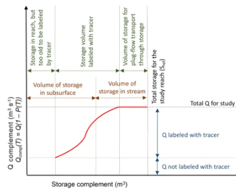
The SAS analysis can be interpreted to yield an under-standing of how storage and discharge are related for the study. The minimum value of the age-ranked discharge com-plement (y axis of Fig. 2) gives the discharge of outflowing water in the channel that was not labeled by the tracer at the upstream end of the study reach within the window of detec-tion. In practice, unlabeled discharge represents some com-bination of (1) down-valley flow entering the segment from upstream and then upwelling and (2) discharge originating from parts of storage that retain tracer for very long periods of time. Finally, while both the discharge and volume sam-pled will scale through the network, each can be normalized

Figure 2.Graphical representation and interpretation the SAS func-tion. Note that the volume of storage in the stream vs. subsurface (orange above) is independent of the SAS analysis and is provided here as an example of integrating the SAS metrics with other knowl-edge about the system.

to a reference value as

fVTOT(T )=

Scomp(T ) Sref

, (27)

fQ,labeled(T )=

Qcomp(T ) Q+Qsub,cap

, (28)

wherefVTOTis the fraction of the total storage volume that was sampled with the tracer, and fQ,labeled is the fraction of the total down-valley discharge that was labeled with the tracer. We also calculated the fraction of the in-stream vol-ume sampled (fVSTR) as

fVSTR=

Scomp(T )

AL . (29)

The SAS approach requires a physically plausible bound-ing by input values. In practice, this means that errors in discharge can cause overestimations of mass recovery (i.e., greater than the mass that was injected), leading to physi-cally impossibleQT(T )values. As a result, we assumed a

typical error of 10 % for dilution gauging (Schmadel et al., 2010). Within that range of discharge values, we calculated the range of physically plausible discharges (i.e., those which yield physically meaningful SAS calculations) and analyzed the midpoint of the plausible range. In the first study us-ing the SAS approach to interpret solute tracers, Harman et al. (2016) found that a similar discharge adjustment was re-quired to define the feasible parameter space.

2.2.4 Long-term storage analysis

Ward et al., 2013c). Dilution gauging at the up- and down-stream ends of each study reach was used to estimate dis-charge (QUSandQDS, respectively, m3s−1). Mass loss along the study reach can be calculated by the difference of the mass injected (MUS, g) andMREC:

MLOSS=MUS−MREC. (30)

Finally, Payn et al. (2009) demonstrate how MLOSS,QUS, andQDScan be used to bound the gross gains and losses of water to the channel through the study reach. We focus here on the case of all losses occurring before all gains, which is the end-member that yields the largest estimates for gross losses (QLOSS,MAX) and gains (QGAIN,MAX), respectively, calculated as

QLOSS,MAX=

MLOSS Rt99

0 Cobs,ds(t )dt

, (31)

QGAIN,MAX=QDS−QUS−QLOSS,MAX. (32) The net change in discharge along the study reach (1Q) is represented by the termsQDS−QUSin the equation above. To compare between reaches, we normalizedMLOSSbyMINJ and normalized the gross gains and losses by QUS. We also calculate gross gains and gross losses,fQGAIN,MAXand

fQLOSS,MAX, as a fraction of the inflow at the upstream end

of the reach.

2.3 Statistical tests

We applied a Mann–Kendall (MK) test to examine relation-ships between the metrics of river corridor exchange and characteristics of geologic setting and hydrologic forcing. The MK test is a nonparametric test used to assess the like-lihood of a monotonically increasing or decreasing trend in a dataset, which we interpret as the presence of a system-atic trend through the river network. The MK test only pro-vides an indication of a relationship’s existence and does not characterize the direction or magnitude of the relationship. Thus, we also calculated Sen’s slope, a nonparametric test to fit a robust linear slope to a dataset by choosing the median of slopes connecting all potential pairs of points. This met-ric was selected because it is less sensitive to outliers than a traditional linear regression and more robust for skewed or heteroscedastic data. Thus, we use the MK test to define the presence or absence of a statistically significant trend (p <0.05) and Sen’s slope to indicate the direction of that trend (positive or negative). We also compare the magnitude of Sen’s slope among and within datasets to estimate the rel-ative sensitivity of selected dependent variables to the same independent variable.

For the synoptic data we also report the coefficient of de-termination (r2) for univariate best-fit power-law regression as an indicator of the predictive power of a parsimonious model fit. The coefficient of determination is commonly in-terpreted as the percent of variance explained by the model.

We selected a power-law regression because most indepen-dent and depenindepen-dent variables span orders of magnitude. We did not test other functional forms as the purpose of this fit is to assess the explanatory power of a simple regres-sion model – comparable to those commonly used to inter-pret field data for identifying relationships between two vari-ables – rather than identify an optimal predictive equation that relates the two variables. Finally, we fit a planar sur-face to each metric as a function of log-transformed base-flow and HYPPOTto approximate the conceptual model pro-posed by Wondzell (2011). We selected a planar surface in log space as the simplest representation of a relationship. We also fit univariate linear relationships to the log-transformed

Q and HYPPOT data for each metric. We emphasize here that our focus was on attesting the conceptual model of Wondzell (2011), not an exhaustive curve- or surface-fitting exercise.

3 Results

3.1 Spatial patterns in hydrologic and geomorphic controls

Overall, all landscape metrics exhibited statistically signifi-cant monotonic trends with one another (MK test,p <0.05). We found expected trends of increasing UAA (Fig. 3a) ve-locity (Fig. 3b) and stream order (Fig. 3c) with discharge. We also found an increasing hydraulic conductivity in the down-network direction (Fig. 3d), which is indicative of sed-iment size and sorting in high-relief headwater landscapes (Brummer and Montgomery, 2003), but opposite to typical low-relief alluvial systems (e.g., Gomez-Velez et al., 2015). Moving from the headwaters to the outlet, we found flatten-ing and widenflatten-ing of the valley with increasflatten-ing discharge and UAA along the network (Fig. 3e, f), increasing stream power (Fig. 3g), and increasing sinuosity (Fig. 3i). This trend re-flects the prevalence of fine material in the upper reaches emplaced by debris flows and coarsening in the downstream direction where stream power increases, thus exporting fines from the system. The result of these trends in valley mor-phology and hydraulic conductivity is an increasing trend inQsub,capin lower network positions (Fig. 3h), indicating the increasing width and K are sufficient to overcome the decreases in slope in generating this relationship. Pairwise Pearson correlation coefficients and Spearman rank correla-tion coefficients are summarized in Supplement Figs. S3 and S4 and Tables S1 and S2.

3.2 River corridor exchange trends with site characteristics

associ-Figure 3.For synoptic data (yellow circles), discharge exhibits a significant, monotonic trend with all other site variables considered (Mann–

Kendall test,p <0.05). Pairwise MK test results for all site characteristic pairs (i.e., allyaxis variables presented above) exhibit significant

trends for all combinations (p <0.05). The solid black line shows the best-fit power-law regression for each panel. Data from unnamed

creek (triangles, Cold creek (squares), WS03 (diamonds), and WS01 (stars) show the repeated injections through baseflow recession for each

headwater catchment. See Supplement Figs. S1 and S2 for similar plots with HYPPOTand UAA on thexaxis.

ated with the well-documented relationship between advec-tive timescale and transient storage (e.g., Ward et al., 2013b; Schmadel et al., 2016a). Despite our efforts to hold advective travel time constant, we still found a trend of increasingtpeak with increasing discharge in our synoptic study (Fig. 4a). Clearly, scaling reach length relative to the wetted channel width (20 wetted channel widths) is not a perfect solution. A perfect experimental design would have resulted in no trend in advective time and provided a window of detection of con-stant size. While a trend was present, we also note that travel time based ontpeakexhibits less variation than discharge (co-efficient of variation 1.00 for travel time compared to 1.49 for discharge). For context, a recent study by Ward et al. (2018b) attempted to control for experiments with 20 min of advec-tive time and accepted a range from 17 to 50 min as compa-rable. Thus, while our selection of study reach lengths was imperfect to achieve identical advective timescales, we con-tend that we have adequately controlled for advective time.

Overall we found significant trends (MK test, p <0.05) between nearly all site characteristics and metrics describ-ing river corridor exchange. Of the 130 pairdescrib-ings investigated, only three (stream order vs.Ldetect, stream order vs.fMAD, sinuosity vs.fQ,labeled) were not significant (Table 3). How-ever, while network-scale trends do exist, we note high site-to-site variation in the dataset as evidenced by the low r2

for the power-law fits (see trend lines in Fig. 4),

representa-tive of the range of explanatory power observed. Across all 130 pairings investigated, we found very little explanatory value in the model fits, with a medianr2 of less than 0.03 (i.e., the variance in the model errors is about 3 % less than the variance in the dependent variable itself). The lack of ex-planatory power for individual variables may indicate that fits based on more complex functional forms and/or multivariate approaches would increase predictive power. We did observe improvedr2for all fits using bothQand HYPPOTcompared to univariate regressions (Table S3).

3.2.2 Fixed-reach vs. synoptic results

Figure 4.Fixed-reach and synoptic data as a function of stream discharge. Statistical likelihood of significant relationships (Mann–Kendall test) and their direction (Sen’s slope) are detailed for all sub-reaches and the synoptic data in Table 3. All trends shown here are significant

(MK test,p <0.05). The coefficients of determination for power-law best fits to synoptic data (black lines) are reported in Table 3. Data

from unnamed creek (triangles, Cold creek (squares), WS03 (diamonds), and WS01 (stars) show the repeated injections through baseflow

recession of each headwater catchment. See Supplement Figs. S5 and S6 for similar plots with HYPPOTand UAA on thexaxis.

ingtpeakwith discharge in the fixed reaches – opposite to the synoptic finding – for 9 of 11 fixed reaches (and steeper Sen’s slope in 9 of 11 fixed reaches). We also found decreasingt99 with discharge in 9 of 11 fixed reaches (all with steeper Sen’s slope than the synoptic) and decreasingLdetectwith discharge in 9 of 11 fixed reaches (all with steeper Sen’s slope than the synoptic). Even with the longer reach lengths, relative to stream size, used in the fixed-reach studies,Ldetectaveraged only∼2.0 m and ranged from a maximum of 10 m to a min-imum of 0.10 m.

With respect to short-term storage, we found increasing

M1with increasing discharge in the synoptic study, but this direction was reflected in only 2 of 11 fixed reaches. Sen’s slope was larger in magnitude for 10 of the 11 fixed reaches, indicating M1 interpreted from the fixed-reach approach is more sensitive to discharge than the synoptic approach. We found overall decreasing CV,γ, andH with increasing

dis-charge in the synoptic study, indicating a decreasing impor-tance of non-advective processes in the downstream direction along the network. The direction of this trend is consistent with seven fixed reaches for CV, two sites forγ, and three sites forH. Regardless of the direction of the relationship, the magnitude of Sen’s slope was larger for all fixed reaches compared to the synoptic study, indicating increased sensi-tivity to discharge relative to the synoptic sites.

T able 4. Sen’ s slope for all dischar ge–metric relationships across fix ed-reach study sites and the synoptic site data. All relationships were significant ( p < 0 . 05) using the Mann–K endall test. The v alues sho wn indicate the direction of the relat ionship based on a Sen’ s slope estimator (“ + ” indicates a direct relationship with dischar ge, and “( − )” indicates in v erse relationship with dischar ge). Slopes were lar ger in magnitude for the fix ed re aches in all cases except Cold Creek sites 12 and 23 for tpeak and Cold Creek site 12 for M 1 , denoted with “

∗”. Catchment

Study reach n Experimental design AD vs. TS Short-term storage rSAS Long-term storage t99 tpeak Ldetect fMAD M 1 CV γ Holdback fQ, labeled fVSTR fVT O T fQg ain , max fQloss , max Unnamed Site 12 6 ( − ) ( − ) + + ( − ) ( − ) + + ( − ) ( − ) ( − ) + ( − ) Site 23 6 ( − ) ( − ) + ( − ) ( − ) ( − ) + + ( − ) ( − ) ( − ) + ( − ) Cold Site 12 5 ( − ) ( − ) ∗ + ( − ) ( − ) ∗ ( − ) ( − ) ( − ) + + + ( − ) + Site 23 5 + ( − ) ∗ ( − ) + + + + + + ( − ) ( − ) + + WS03 Site 12 5 + ( − ) ( − ) ( − ) + ( − ) + + + ( − ) + ( − ) + Site 23 5 ( − ) ( − ) + + ( − ) ( − ) + ( − ) ( − ) ( − ) + + ( − ) Site 34 5 ( − ) + + + ( − ) ( − ) ( − ) ( − ) ( − ) ( − ) ( − ) ( − ) ( − ) WS01 Site 12 3 ( − ) ( − ) + ( − ) ( − ) ( − ) + + ( − ) + + + ( − ) Site 23 2 ( − ) + + ( − ) ( − ) + + + + + ( − ) ( − ) + Site 34 2 ( − ) ( − ) + ( − ) ( − ) + + + + ( − ) ( − ) ( − ) + Site 45 3 ( − ) ( − ) + ( − ) ( − ) + + + + + ( − ) ( − ) + HJ A synoptic ( Q ) 46 ( − ) + + ( − ) + ( − ) ( − ) ( − ) + ( − ) ( − ) ( − ) ( − ) HJ A synoptic (HYP PO T ) 46 ( − ) ( − ) ( − ) ( − ) ( − ) ( − ) + + ( − ) + + + +

was larger for the fixed reaches than the synoptic study for

fMAD,fQgainmax, andfQlossmax.

The SAS analysis revealed decreasing sampling of the to-tal storage zone (fVtot) with increasing discharge but

increas-ingfQ,labeledwith discharge for the synoptic study. Together,

these results indicate that increasing discharge in synoptic experiments resulted in sampling a larger fraction of the wa-ter exiting the reach but smaller total volume of storage. Put another way, experiments in locations with higher discharge were more likely to measure storage in (or proximal to) the stream channel at the expense of measuring more distal flow paths and less-connected storage. For the fixed-reach studies, we found decreasingfVtotandfQ,labeledin seven and six of the 11 reaches, respectively. In all cases, the magnitude of Sen’s slope was larger for the fixed reaches than the synoptic study.

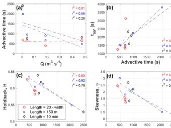
3.3 Selection of study reach length across the network For the injections that specifically tested the study reach length, we found the most consistent advective timescales were obtained by scaling reach length to 20 times wet-ted channel width (Fig. 5). Ranges of advective timescales were 25.2 min for the fixed-length approach, 27.2 min for the fixed-timescale approach, and 4.8 min for the 20× wet-ted channel width approach (Fig. 5a). It is notable that our estimates of a 10 min advective time were reasonably accu-rate for the three highest-discharge reaches, but the lowest-discharge replicate primarily drives the visually steep trend. We hypothesize that a better estimate of advective velocity – such as using a dye tracer rather than following debris or a longer length scale of integration – may have improved that estimate. Fort99, ranges for the 10 min and 150 m approaches are about 29 % and 22 % larger, respectively, than the 20× wetted channel width approach (Fig. 5b). Differences are even more striking for other parameters, with the 10 min and 150 m study designs yielding 147 % and 93 % larger ranges forH compared to the 20×wetted channel width approach (Fig. 5c). Similarly, the 10 min and 150 m approaches result in ranges ofγthat are 96 % and 101 % larger than the ranges using the 20×wetted channel width approach (Fig. 5d).

4 Discussion

4.1 How do discharge and local geomorphic setting modulate river corridor exchange?

Figure 5. Comparison of fixed-reach (150 m), adaptive-reach length (20 wetted channel widths), and fixed-advective-time (10 min)

ap-proaches for standardization of stream solute tracer studies.(a)Control of advective time across 4 stream orders. Additional panels show the

observations and a best-fit linear regression for(b)longest detection timescale,(c)holdback, and(d)skewness in relation to the advective

time of the study. Best-fit linear regressions are shown as dashed lines in each panel.

andfQLOSS,Maxgenerally decrease in parameter value with

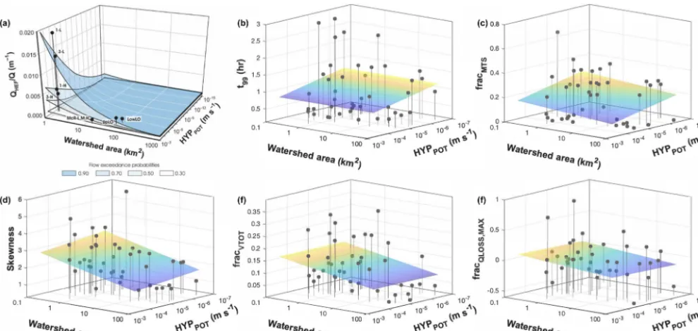
increase in catchment area (Fig. 6b–f). This finding is in agreement with the conceptual model of Wondzell (2011), who predictedQHEF/Qwould decrease as drainage area in-creased. We did find an increasing fraction of total discharge sampled in higher-discharge locations (Fig. 4c), but the over-all trend indicates that QHEF does not grow as rapidly as Q, moving downstream along the network. This is consis-tent with findings of decreased river corridor exchange in network locations with larger discharge (e.g., Covino et al., 2011; Ward et al., 2013c).

Two explanations have been posed relating river corridor exchange to time-variable baseflow in a given study reach, both of which result in less exchange under higher-discharge conditions. First, many conceptual models would predict that increasing baseflow is associated with increasing groundwa-ter discharge to the stream, resulting in compression of hy-porheic zones and decreased river corridor exchange (Hak-enkamp et al., 1993; Hynes, 1983; Palmer, 1993; Vervier et al., 1992; White, 1993). Second, exchange may change little during storm events because, under a wide range of discharge conditions, the effect of the geomorphic features driving exchange flows may be relatively static (Ward et al., 2017b). Thus, if QHEF is relatively static, as Q increases the relative amount of relative exchange (QHEF/Q) will de-crease. Both explanations appear logical and suggest that river corridor exchange should change systematically with

discharge. However, we did not find a consistent pattern in our synoptic field study. Rather, of the diverse array of met-rics used to characterize river corridor exchange in the synop-tic study, some increased and some decreased with increasing discharge. We found similarly contradictory results among our fixed-reach studies. For example, only two of 11 fixed reaches exhibited the expected negative relationship based on skewness (one indicator ofQHEF/Q) and discharge (Ta-ble 4).

4.2 Heterogeneity in the river network

direc-Figure 6.Comparison of(a)conceptual model of river corridor exchange (reprinted from Wondzell (2011) with permission) and findings from this study including a best-fit planar surface fit to the synoptic data for each panel (dots show the data points, and stems extend to

the bottom X–Y plane to aid in visualization; planar surface light-to-dark shading indicates high to low for thezaxis variable). Panels

show trends for a subset of variables representing(b)experimental design,(c)separation of advection–dispersion from transient storage,

(d)short-term storage,(e)StorAge Selection, and(f)long-term storage. Goodness of fit and slopes for each fit are summarized in Table S3.

tion. We note, however, that our studies only spanned about 4 orders of magnitude in hyporheic potential while the model of Wondzell (2011) visualizes a range that spans 14 orders of magnitude. Our study is also limited to the upper end of the range in hyporheic potential depicted by Wondzell (2011).

Our dataset also showed substantial spatial heterogeneity in all metrics along the river corridor. While the conceptual model of Wondzell (2011) does not expressly disallow such heterogeneity, the data points he used to develop the con-ceptual model suggest very uniform changes with watershed area and little change in hyporheic potential from 2nd- to 5th-order reaches within the same mountain stream network studied here. Our results suggest that the influence of reach-scale heterogeneity among sites may be as large as, or even larger than, the expected systematic changes with watershed size. We also note that our results may differ from those of Wondzell (2011) for methodological differences. First, Wondzell (2011) based his estimates of K from extensive well networks at each of his sites, using the geometric mean of all wells – including many wells on the floodplain adja-cent to the stream as well as piezometers installed through the streambed. This study estimatedK from a single 50 cm deep piezometer located in the channel thalweg, and the data of Wondzell (2011) show that K is higher in piezometers inserted into the shallow streambed than in floodplain sedi-ment adjacent to the stream. Second, Wondzell (2011) used numerical simulations from groundwater flow models to

cal-culateQHEF, whereas exchange metrics in this study were derived from stream solute tracer injections. Solute injections are sensitive to both surface (in-stream) and subsurface tran-sient storage, and metrics derived from these studies have a known bias toward the shortest transit times (Harvey et al., 1996; Wagner and Harvey, 1997; Harvey and Wagner, 2000), a bias that is clearly evident in our data. For example, the longest timescale flow path detectable, interpreted fromt99, in our study reaches ranged from about 8 min to 2.8 h. In contrast, the simulations of Wondzell (2011) included flow paths with up to 10 d transit times. However, cell sizes in the finite-difference grids used in his models limited the shortest flow paths that could be simulated, so his estimates ofQHEF should underrepresent the very shortest flow paths present within the reach.

in most reaches, but it is unclear what the mechanisms or timescales of exchange were for the storage locations mea-sured. Overall, this unique basin-scale dataset does not ap-pear to support the conceptual model of Wondzell (2011) with respect to hyporheic potential, but it does not disprove it either due to the limitations in methods, and clustering on only the highest end of the axis likely biased our results. Still, we suggest local-scale processes specific to individual sites may overwhelm basin-scale trends and limit the abil-ity of continuum-based conceptual models, such as that of Wondzell (2011), to predict local-scale hyporheic and river corridor exchange dynamics.

4.3 Can space-for-time or time-for-space relationships be used to transfer findings based on reach-scale characteristics?

Transferability of findings in space or time relies upon two assumptions, both of which are necessary conditions for reli-able prediction. First, transferability requires that the process of interest varies systematically with at least one observable variable at the study and predicted sites. In our case, this re-quires the relationship between discharge and river corridor exchange to be measurable and robust, commonly judged on the basis of a goodness-of-fit metric for a regression. Trans-ferability also requires that the functional form established from the observations holds for the conditions that are being predicted. In the temporal domain this is most commonly in-terpolation in time to predict river corridor exchange under a discharge condition that was not actually observed (e.g., Har-man et al., 2016; Ward et al., 2018a). In the spatial domain, this transferability strategy may manifest as interpolation be-tween observed sites (e.g., Covino et al., 2011; Mallard et al., 2014) or extrapolation to sites that are morphologically sim-ilar, such as extending findings from one headwater site to make predictions in an adjacent basin or another stream reach (e.g., Jencso et al., 2011; Covino et al., 2011; Stewart et al., 2011). This approach assumes that the relationship holds be-cause the observational and predicted sites are similar. How-ever, we find that there is substantial variation among sites, particularly when reaches of similar size yield opposing re-lationships with explanatory variables (Tables 2, 3).

Overall, we conclude that discharge alone is a poor predic-tor of river corridor exchange in mountain stream networks due to heterogeneity in reach-scale geomorphic settings and should not be used as the sole basis for spatial or tempo-ral extrapolation of findings. We found opposing relation-ships between river corridor exchange and discharge through space (synoptic approach) and time (fixed-reach approach). For all metrics considered, at least 18 % (two of 11) of the intensively studied fixed reaches had trends opposite of what would be predicted from the one-time sampling of the syn-optic study. Moreover, the opposing trends were always lo-cated across at least two different landform types, and there were examples of within-landform-type disagreement for

ev-ery metric considered. Furthermore, the regressions we de-veloped indicated that there was substantial inter-site hetero-geneity overriding the observed network-scale trends. These findings are useful for identifying best practices to ultimately develop better scaling relationships to predict river corridor exchange as a function of hydrologic forcing and geomorphic setting from headwaters to oceans. For example, intensively studying a small number of study reaches is not indicative of the conditions occurring across an entire basin, even at the scale of our 5th-order basin. We further develop suggestions for best practices and considerations in the next section. 4.4 Best practices to measure and interpret

exchange–discharge relationships

Stream solute tracers are perhaps the empirical method most frequently used to measure river corridor exchange. Given the relative ease and low cost of this method, it is unsur-prising that many studies have used solute tracer studies un-der different discharge conditions to assess relationships be-tween discharge and river corridor exchange. For example, some studies repeat solute injections in a fixed reach under a range of discharge conditions during different seasons (e.g., Zarnetske et al., 2007; Ward et al., 2018b), during baseflow recession (e.g., Payn et al., 2009; Ward et al., 2012), or during storm events (e.g., Ward et al., 2013b; Dudley-Southern and Binley, 2015). Still others use spatial replication at multiple sites within a network to construct a relationship that can be used to predict behavior for unstudied reaches during a single discharge condition (e.g., Jencso et al., 2011; Covino et al., 2011; Stewart et al., 2011). However, limitations of stream solute tracers are well documented in the literature as men-tioned above (Harvey et al., 1996; Wagner and Harvey, 1997; Harvey and Wagner, 2000; Drummond et al., 2012; Kelleher et al., 2013; Ward et al., 2017a).

mechanistic understanding of the river corridor or suffer from confirmation bias. Therefore, we detail two best practices for conducting and interpreting stream solute tracer tests for those seeking to do as we have attempted in this study. 4.4.1 Best practice 1: control for advective timescales

instead of reach length

The most common paradigm in stream solute tracer studies is to use a fixed-length study reach and hold length constant to compare different reaches (e.g., Payn et al., 2009; Covino et al., 2011) or to compare different discharge conditions at a single reach of fixed length (e.g., Schmadel et al., 2016a; Ward et al., 2013a). The implicit logic is that by fixing the reach length, the same morphologic features interact with the tracer and allow the researcher to measure changes in the same processes. However, this is only true in the case where the same suite of flow paths can be detected. When advective timescales decrease, the window of detection (i.e., the longest timescale flow path that can be detected) should decrease in response (e.g., Schmadel et al., 2016a). As a re-sult, the fixed reach causes systematic bias in the tracer ex-periment. Higher discharges will have smaller windows of detection, biasing the results toward shorter timescale flow paths compared to low-discharge injections.

Based on our findings (Fig. 5), plus the well-documented interaction of advective timescale with river corridor ex-change measured with solute tracers, we strongly rec-ommend experimental designs that control for advective timescale. We suggest that an upstream location be estab-lished and fixed in space. Then the length of the study reach should be determined, either by scaling by channel width (e.g., 20 times the wetted channel width) or by using a dye tracer to measure advective velocity over a length equal to perhaps 10 wetted channel widths, and then using advective velocity to calculate a study reach length that provides uni-form advective travel times in all reaches studied.

When tracer injections are designed to provide uniform advective travel times, the resulting study reach lengths will be longest in the largest streams and/or at times of high dis-charge; reaches will be shortest under low-discharge condi-tions. It is critical that the shortest reach length still encom-passes a length of stream that is sufficient to integrate rep-resentative variation in morphology of the study system. If reaches are too short, high reach-to-reach variability will be generated by one or a few morphologic features and these local conditions are likely to dominate comparisons among reaches and make it difficult to discern the influence of changing hydrologic conditions. It will be difficult to deter-mine a length-scale long enough to integrate the full range of morphologic features present in any given stream. Schmadel et al. (2014) suggested that a morphologically representa-tive reach could be determined by knowing the length of spatial autocorrelation of morphologic features, but this re-quires substantial effort to survey or map the study reach

prior to conducting a tracer test. A less effort-intensive but more equipment-intensive approach would be to place mul-tiple sensors in the study reach (perhaps 10, 20, 35, 50, 75, and 100 wetted channel widths) and select most appropriate downstream breakthrough curves to compare based on simi-larity of advective timescales after conducting the tracer test. It is also essential that measures of the advective timescale and window of detection be reported for each tracer test. For slug injections these would includetpeak and t99. For con-stant rate injections these would be time to the steepest point on the rising limb, time to median arrival (M1), and time to achieve plateau. TheLdetectestimates should also be reported and these should be based on time to achieve plateau as that indicates when the tracer has traveled the full length of all measurable flow paths and only tracer-labeled water is being returned to the stream. These metrics describing the advec-tive timescale are necessary both to confirm that comparisons among reaches in any given study are valid and to facilitate comparisons of results among published studies.

We acknowledge here that the steps we have recom-mended above will require substantial time and analysis to design a stream tracer experiment. However, we contend this additional work is necessary to maximize the interpretability of the data and enable meaningful comparison across space and time.

4.4.2 Best practice 2: critical evaluation of which flow paths may have been measured by the experiment One persistent limitation of interpreting stream solute trac-ers is the inability to know which flow paths and features were actually measured in the study reach. While additional observations in storage zones have been attempted via mon-itoring wells or geophysical imaging, multiple studies show that solute observed in the storage zone itself is not necessar-ily meaningful, as the stream breakthrough curve integrates only a subset of flow paths (Ward et al., 2010a, 2017b, Toran et al., 2012, 2013). Briggs et al. (2009) suggest additional measurements in the surface storage domain may allow for parsing surface from subsurface transient storage. However, this approach relies upon measurement of a representative in-stream storage zone and interpretation via the transient stor-age model, which is known to be limited in identifiability of parameters and transferability to other sites (e.g., Kelleher et al., 2013; Ward et al., 2017a).

been observed. For example, in previous studies of a small stream in the HJA basin (WS01, Fig. 1), where extensive penetration of the tracer into the subsurface was documented across a 10+m wide valley bottom (Voltz et al., 2013; Ward et al., 2017b), the longest flow paths detected by a tracer re-turning to the stream still only averaged 0.21 m (range 0.004 to 1.2 m) compared to overall reach lengths of tens of meters. This means that these studies were measuring in-stream stor-age and only the shortest and fastest subsurface flow paths – not integrating all the exchange in the valley bottom.

The SAS approach implemented in this study provides some valuable additional contextual information about the storage volume and discharge that informs interpretation of findings. For example, our synoptic study labeled an aver-age of 86 % of the outflowing discharge in the surface chan-nel (range 57 % to 95 %). Still, this equated to having only sampled an average of 12 % of the total storage volume in the reach (range 0.3 % to 35 %), suggesting a bias toward in-stream storage. This bias is confirmed by the realization that, on average, only 18 % of tracer mass was involved in transient storage (range 0 % to 69 %). Hence, the SAS ap-proach gives us additional insights and reveals biases in the tracer methods. Altogether, this study clearly indicates that multiple data collection, analysis, and modeling techniques are needed to develop scaling relationships representative of river corridor exchange across varying hydrologic forcing and geomorphic settings.

5 Conclusions

We set out to leverage novel datasets collected across a 5th-order basin to test the existence of systematic relationships linking river corridor exchange with temporal variation in discharge, spatial patterns in discharge, and local geomorphic setting. We specifically intended to use these data to critically test the conceptual model of Wondzell (2011) (Fig. 6a). We found systematic patterns, namely decreases in several indi-cators of river corridor exchange with increasing discharge in space (i.e., moving downstream in the network), confirm-ing this part of the Wondzell (2011) conceptual model. The model of Wondzell (2011) predicts the same trend for in-creasing baseflow discharge in time, but we found both direct and inverse relationships between river corridor exchange and discharge at fixed reaches under varied baseflow con-ditions. These findings reflect a high degree of heterogene-ity on a reach-to-reach basis in space, likely overwhelm-ing or obscuroverwhelm-ing river corridor exchange patterns that might emerge in more spatially continuous and larger-scale assess-ments, which would be a better test of the Wondzell (2011) model. Importantly, we document consistent trends with dis-charge that have low explanatory power (lowr2) despite be-ing statistically significant in their direction, indicatbe-ing that we have little predictive power. Moreover, our findings re-veal the challenges that must be addressed to design and

interpret stream solute data among sites or discharge con-ditions. Finally, we did not confirm the predicted pattern of Wondzell (2011) with respect to local hyporheic potential at a site, which may have been confounded by integration of both surface and hyporheic storage by the stream solute tracers or by local-scale heterogeneity not captured in our reach-scale site characterization. Collectively, the larger Sen’s slopes for the fixed reaches, when compared across variable hydrologic conditions, may indicate more temporal variation at a site through the season than there is through the network un-der the single baseflow condition. This means that caution is needed in applying synoptic sampling approaches across time when studying river corridor exchange conditions in a river network.

This study documented the interaction between advective travel times and measurement of river corridor exchange with solute tracers. Our synoptic study design controlled for this complication by scaling study reach lengths based on wet-ted channel width. For future studies focused on exchange– discharge relationships, we suggest two best practices. First, we suggest controlling for advective time to measure consis-tent timescales of storage processes and limit artifacts that are due to limitations of solute tracer studies. Second, we suggest analyses that focus on the fractions of storage vol-ume and outflow that were labeled with tracer to provide context for interpreting recovered time series. We also note that many previous studies have relied upon small sample sizes and focused on singular explanatory variables of in-terest considered in isolation. We suggest this is primarily descriptive, and we conclude that consideration of multiple interacting controls will be necessary to achieve predictive understanding of river corridor exchange across varying hy-drologic forcing and geomorphic setting from headwaters to large river networks.

Finally, we underscore that a one-time synoptic sampling campaign does not address local-scale variability that is cre-ated by variable discharge conditions, nor does extensive study of a single reach provide data that are reflective of vari-ation in space in the river network. In short, space-for-time and time-for-space substitutions based on the methods used in our study are not a reliable basis for transferability or pre-diction.

Data availability. All data used in this study are

archived in the Consortium of Universities for the

Ad-vancement of Hydrologic Science, Inc. (CUAHSI)

HydroShare data repository, publicly accessible at