Hydroclimatic control on suspended sediment dynamics of a regulated Alpine catchment: a conceptual approach

https://doi.org/10.5194/hess-22-3421-2018 © Author(s) 2018. This work is distributed under the Creative Commons Attribution 4.0 License.

Hydroclimatic control on suspended sediment dynamics of a

regulated Alpine catchment: a conceptual approach

Anna Costa, Daniela Anghileri, and Peter Molnar

Institute of Environmental Engineering, ETH Zurich, 8093 Zurich, Switzerland Correspondence:Anna Costa (costa@ifu.baug.ethz)

Received: 7 January 2018 – Discussion started: 9 January 2018 Accepted: 26 May 2018 – Published: 22 June 2018

Abstract. We analyse the control of hydroclimatic factors on suspended sediment concentration (SSC) in Alpine catch-ments by differentiating among the potential contributions of erosion and suspended sediment transport driven by erosive rainfall, defined as liquid precipitation over snow-free sur-faces, ice melt from glacierized areas, and snowmelt on hill-slopes. We account for the potential impact of hydropower by intercepting sediment fluxes originated in areas diverted to hydropower reservoirs, and by considering the contribu-tion of hydropower releases to SSC. We obtain the hydro-climatic variables from daily gridded datasets of precipita-tion and temperature, implementing a degree-day model to simulate spatially distributed snow accumulation and snow– ice melt. We estimate hydropower releases by a conceptual approach with a unique virtual reservoir regulated on the ba-sis of a target-volume function, representing normal reservoir operating conditions throughout a hydrological year. An It-erative Input Selection algorithm is used to identify the vari-ables with the highest predictive power for SSC, their ex-plained variance, and characteristic time lags. On this ba-sis, we develop a hydroclimatic multivariate rating curve (HMRC) which accounts for the contributions of the most relevant hydroclimatic input variables mentioned above. We calibrate the HMRC with a gradient-based nonlinear opti-mization method and we compare its performance with a tra-ditional discharge-based rating curve. We apply the approach in the upper Rhône Basin, a large Swiss Alpine catchment heavily regulated by hydropower. Our results show that the three hydroclimatic processes – erosive rainfall, ice melt, and snowmelt – are significant predictors of mean daily SSC, while hydropower release does not have a significant ex-planatory power for SSC. The characteristic time lags of the hydroclimatic variables correspond to the typical flow

concentration times of the basin. Despite not including dis-charge, the HMRC performs better than the traditional rat-ing curve in reproducrat-ing SSC seasonality, especially dur-ing validation at the daily scale. While erosive rainfall de-termines the daily variability of SSC and extremes, ice melt generates the highest SSC per unit of runoff and represents the largest contribution to total suspended sediment yield. Finally, we show that the HMRC is capable of simulating climate-driven changes in fine sediment dynamics in Alpine catchments. In fact, HMRC can reproduce the changes in SSC in the past 40 years in the Rhône Basin connected to air temperature rise, even though the simulated changes are more gradual than those observed. The approach presented in this paper, based on the analysis of the hydroclimatic con-trol of suspended sediment concentration, allows the explo-ration of climate-driven changes in fine sediment dynam-ics in Alpine catchments. The approach can be applied to any Alpine catchment with a pluvio-glacio-nival hydrologi-cal regime and adequate hydroclimatic datasets.

1 Introduction

mass wasting events such as debris flows and landslides (e.g. Caine, 1980; Dhakal and Sidle, 2004; Guzzetti et al., 2008; Leonarduzzi et al., 2017), which can mobilize large amounts of fine sediment (e.g. Korup et al., 2004; Bennett et al., 2012) and result in very high suspended sediment concentrations in the receiving streams. Together with erosional processes along hillslopes, which are strongly related to rainfall inten-sity (e.g. Van Dijk et al., 2002), precipitation events may also enhance channel and bank erosion through increased discharge. Ice melt (IM) is responsible for high concentra-tions of fine sediment produced with a variety of glacial ero-sion processes (Boulton, 1974). Ice melt may substantially increase suspended sediment concentration in glacially fed streams by entraining and transporting fine sediment previ-ously stored in subglacial networks and paraglacial environ-ments (Aas and Bogen, 1988; Gurnell et al., 1996; Lawler and Dolan, 1992). Snowmelt-driven overland flow (SM) gen-erates hillslope erosion and potentially affects channel and bank erosion by contributing to streamflow. This hydrocli-matic forcing is important in Alpine environments where snowmelt can produce high hillslope runoff and be a major contributor to channel discharge (e.g. Grønsten and Lundek-vam, 2006; Ollesch et al., 2006; Konz et al., 2012). Due to the diversity of the erosion and transport processes (e.g. ero-sion driven by overland flow, mass wasting events) and the variety of sediment sources involved (e.g. hillslopes, chan-nels, glaciers), sediment fluxes generated by these three hy-droclimatic variables are expected to contribute to suspended sediment dynamics in a complementary way, both in terms of magnitude and timing.

In addition to natural hydroclimatic forcings, human ac-tivities potentially contribute to altering sediment dynamics, e.g. by changes in land use (e.g. Foster et al., 2003) and sediment storage in reservoirs (e.g. Syvitski et al., 2005). In Alpine environments, it is water impoundment and flow reg-ulation due to hydropower production especially which may substantially influence the suspended sediment regime (e.g. Anselmetti et al., 2007). The impacts of hydropower oper-ations on suspended sediment dynamics may vary substan-tially between catchments, depending on the specific features of the hydropower system (e.g. reservoir trapping efficiency, hydropower operations), and on the catchment characteris-tics (e.g. amount and grain size distribution of the eroded sediment, seasonal pattern of sediment production). Here, we focus on the two main effects of hydropower operations: sediment trapping in reservoirs and temporary sediment stor-age behind water diversion infrastructures (intakes), which may substantially reduce the amount of sediment delivered to downstream reaches and/or significantly alter the timing of sediment release to the river network (e.g. Vörösmarty et al., 2003; Finger et al., 2006; Gabbud and Lane, 2016; Bakker et al., 2018). Despite sediment trapping, water released from hydropower (HP) reservoirs may carry suspended sediment either previously stored in the reservoirs or entrained along the downstream channels.

In the context of environmental change, it is important to understand how the sediment regime has changed and what the relative role of different hydroclimatic forcings may have been. There are examples of studies which demonstrated al-terations in suspended sediment yields driven by changes in land use, climate, or by disturbances such as wildfires, earth-quakes, and flow impoundments (e.g. Loizeau and Dominik, 2000; Foster et al., 2003; Dadson et al., 2004; Yang et al., 2007; Horowitz, 2010; Costa et al., 2018). These changes are normally addressed by calibrating different sediment rat-ing curve models, which express suspended sediment con-centration as a power function of discharge, for different sediment supply regimes and by making the parameters of the rating curves time-dependent (e.g. Syvitski et al., 2000; Yang, 2007; Hu et al., 2011; Huang and Montgomery, 2013; Warrick, 2015). However, these approaches do not explic-itly address the sources of sediment and their activation by different hydroclimatic forcings and are limited to using dis-charge as a predictor. As a result the hydroclimatic causality of changes in suspended sediment concentration in such anal-yses remains elusive. The approach proposed in this paper accounts explicitly for the hydroclimatic and hydropower ac-tivation and deacac-tivation of different sediment sources, with the aim to identify their predictive power in estimating sus-pended concentration even without using discharge.

Our main objectives are (1) to explore the role played by the hydroclimatic variables erosive rainfall, ice melt, snow-melt, and the hydropower release, in controlling suspended sediment concentration of an Alpine catchment, and (2) to analyse long-term, climate-driven changes in suspended sed-iment concentration on the basis of a conceptual, data-driven approach accounting separately for the contribution of ero-sive rainfall, ice melt, snowmelt, and hydropower releases.

the lithological unit more affected by hydropower is under-represented at the outlet of the catchment, suggesting the im-pact of water impoundment on the sediment budget of the basin. In addition, alterations of suspended sediment concen-tration entering Lake Geneva have been observed in the re-cent past and attributed to human impacts (Loizeau and Do-minik, 2000; Loizeau et al., 1997) and changes in climatic conditions (Costa et al., 2018).

The paper is organized as follows: Sect. 2 describes the data pre-processing, the hydrological modelling procedure to obtain the hydroclimatic variables (ER, IM, SM), the ap-proach to obtain the hydropower releases (HP), and the anal-ysis performed to infer their link to suspended sediment con-centration; Sect. 3 presents the upper Rhône Basin and the data used in our analysis; Sect. 4 reports the main results which are discussed in Sect. 5; and Sect. 6 concludes the pa-per by summarizing the main findings.

2 Methods

To analyse the role of hydroclimate on the suspended sedi-ment regime of a catchsedi-ment regulated by hydropower reser-voirs, we first divide the catchment into two distinct areas: (1) the area which contributes to the runoff accumulated in hydropower reservoirs (regulated area), including the frac-tion of the catchment draining directly into the reservoirs and the fraction connected to the reservoirs through tunnels and pumping stations, and (2) the remaining area, which naturally flows to the river network (unregulated area). We assume that the sediment fluxes originated in the unregulated area con-tribute directly to SSC at the outlet of the catchment, while sediment fluxes generated in the regulated area are diverted into the reservoirs and later totally or partially released ac-cording to hydropower operations. Finally, we estimate the contribution to SSC at the outlet of the catchment of sedi-ment fluxes originated in the unregulated area by ER, IM, and SM, and of sediment fluxes carried by water released from the reservoirs during hydropower operations.

Our methodology consists of four main steps:

1. We derive mean daily SSCt, ERt, SMt, IMt, and

HPtdatasets. Mean daily SSCt at the outlet of the

catchment is derived from continuous measurements of turbidity (Sect. 2.1), the hydroclimatic input variables mean daily ERt, SMt, and IMt are derived from

spa-tially distributed snowmelt and ice melt models, and the mean daily water releases from hydropower reservoirs HPt are derived by a conceptual approach based on a

unique virtual reservoir, which is intended to model the cumulative effect of multiple reservoirs, when present in the catchment, and a target volume function (Sect. 2.2). 2. We use an Input Variable Selection algorithm to identify the variables with the highest predictive power for SSCt

and we estimate their characteristic time lags (Sect. 2.3).

3. We calibrate and validate a rating curve accounting for the variables identified in the previous step (hydrocli-matic multivariate rating curve – HMRC), and we eval-uate the contribution of each hydroclimatic and hy-dropower component to SSCt (Sect. 2.4).

4. We apply the HMRC to simulate 40-year-long time se-ries of SSCt at the outlet of the catchment to

investi-gate the impact of changes in climatic conditions on sus-pended sediment dynamics, and we compare simulated values with observations obtained with a traditional rat-ing curve (RC) based on discharge only (Sect. 2.5).

2.1 Estimate of daily suspended sediment concentration

The specific operations described in this and the following paragraphs strongly depend on the data availability for the case study under consideration. In the following, we describe the operations we carried out for the upper Rhône Basin, but we also comment about the applicability of these and alter-native operations to other catchments.

after a logarithmic transformation of the variables:

SSC=a0·NTUb0. (1)

For the back-transformation from the logarithmic to the linear scale, we applied the correction factor proposed by Duan (1983). Finally, we compute mean daily NTU values from continuous measurements of turbidity, and we use the SSC–NTU relation (Eq. 1) to estimate mean daily SSC. 2.2 Hydroclimatic data modelling

Datasets of the hydroclimatic variables ER, IM, and SM need to be derived by hydrological modelling. The choice of the model should be driven by the data availability for calibra-tion and the required accuracy of the simulated outputs. In our case, we use a conceptual and spatially distributed model of snowmelt and ice melt driven by spatially distributed pre-cipitation and temperature (Costa et al., 2018). We use grid-ded datasets of mean daily precipitation and mean, maxi-mum, and minimum daily air temperature to divide precipi-tation into rainfall and snowfall on the basis of a temperature threshold. We model ice and snow accumulation and melt-ing with a degree-day approach (e.g. Hock, 2003). Ice melt occurs only on glacier cells that are snow-free. Likewise, ero-sive rainfall occurs only on snow-free hillslope cells. We set temperature thresholds for snow–rain division (1◦C) and for snowmelt and ice melt initiation (0◦C) based on the literature and on previous studies (e.g. Fatichi et al., 2015; Costa et al., 2018), while we calibrate melt factors with satellite-derived snow cover (Moderate Resolution Imaging Spectroradiome-ter, MODIS) and with discharge measured at different loca-tions in the catchment. We first calibrate the snowmelt rate from snow cover maps by spatial statistics that measure the grid-to-grid matching of the model. Second, we calibrate the ice melt rate on the basis of discharge measured at the outlet of two highly glaciated subcatchments. For more details on the hydrological model description and calibration see Costa et al. (2018). Finally, we sum the spatially distributed hy-droclimatic variables over the regulated and unregulated ar-eas and we obtain respectively mean daily ERHP_t , IMHP_t , and SMHP_t along with ERt, SMt, and IMt.

We represent all the hydropower reservoirs operating in the catchment with a unique virtual reservoir, because data of water releases from individual reservoirs are seldom avail-able. The release from the virtual reservoir is estimated on the basis of a target-volume function which represents the reservoir operations in normal conditions. For each day of the year, the hydropower release from the virtual reservoir HPt+1 within the interval from day t to day t+1 is

esti-mated as the difference in the reservoir storage and the target volume, when positive, zero otherwise. The reservoir storage Vt+1is finally computed on the basis of the mass balance:

Vt+1=Vt+It+1−HPt+1, (2)

whereIt+1 represents the inflow into the virtual reservoir

within the interval from daytto dayt+1.

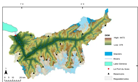
To derive the capacity of the virtual reservoir, we consider the 13 largest reservoirs operating in the Rhône catchment. A list of the reservoirs with their retention capacity is reported in Table S1 of the Supplement, while their spatial location is shown in Fig. 1. We compute the target-volume functions of each individual reservoir by averaging observed storage time series for reservoirs when observations are available and by adopting normalized reference curves within the individual reservoir regulation range otherwise (see Fatichi et al., 2015 for the full details). We then compute the target-volume tion of the virtual reservoir by adding the target-volume func-tions of each individual reservoir and by scaling the sum to the total annual inflow. We compute the daily inflow It in

Eq. (2) as the sum of the three hydroclimatic fluxes, erosive rainfall, ice melt, and snowmelt, generated over the regulated area:

It=ERHPt +IMHPt +SMHPt . (3)

It should be noted thatIt represents direct potential runoff

from the regulated area without accounting for evapotranspi-ration and infiltevapotranspi-ration losses. We therefore scale the capacity of the virtual reservoir, to obtain reservoir seasonal dynam-ics resembling the available observations. For the scaling, we assume the minimum volume of the virtual reservoir equal to zero, and the maximum volume equal to 70 % of the total an-nual inflow into the reservoirs, which roughly corresponds to the average ratio between storage capacity and total annual inflow. The procedure described above implies that all reser-voirs of the catchment are regulated following the same oper-ational rule driven by the seasonality of inflow, i.e. an annual cycle of drawdown during winter and refill during spring and summer. Due to their geographical proximity, the similar el-evation, and the available observations, this assumption can be considered realistic. We validate the hydropower opera-tions model by comparing the mean daily normalized values of simulated hydropower releases of the virtual reservoir and observations from Mattmark, a reservoir with a volume ca-pacity of 108m3located in the upper part of the catchment. Although our hydropower operations model is relatively sim-ple, the comparison shows a good agreement with the obser-vations (Fig. S1 of the Supplement).

2.3 Input variable selection algorithm

We apply the Iterative Input Selection (IIS) algorithm (Galelli and Castelletti, 2013) to (1) select which variables play a significant role in predicting SSCt, (2) quantify their

relative importance, and (3) identify the time lags of the sed-iment flux associated with each selected variable. The IIS al-gorithm selects the most relevant input variables, among a set of candidate input variables (in our case mean daily ERt−l,

SMt−l, IMt−l, and HPt−lat different time lagsl), to predict a

cal-ibrates and validates a series of regression models consider-ing different sets of input variables and selectconsider-ing the ones that display the best model performances. The algorithm adopts extremely randomized trees, or “Extra-Trees” (Geurts et al., 2006), as regression models, because they allow nonlinear re-lations between input and output variables to be dealt with in a computationally efficient way. The Extra–Trees regression is based on a recursive splitting procedure, which partitions the dataset into subsamples containing a specified number of elements. This splitting procedure is performed several times by randomizing both the input variable and the cut-point used to split the sample, in order to minimize the bias of the final regression (for more details see Geurts et al., 2006).

The IIS algorithm is based on an iterative procedure, which allows for the ranking of the candidate input variables according to their significance in explaining the output vari-able on the basis of the coefficient of determinationR2of the underlying regression model. At the first iteration, regression models are identified and the candidate variable leading to the best model performance is selected. At subsequent iter-ations, the original output variable (i.e. SSCt) is substituted

with the residual of the model computed at the previous it-eration. This ensures that candidate input variables that are highly correlated with the selected one are discarded and, thus, reinforces the ability of the IIS algorithm against the selection of redundant and cross-correlated input variables (Galelli and Castelletti, 2013). Because of the relatively short duration of our dataset and the marked seasonal pattern that characterizes the considered candidate input variables and output variable, we randomly shuffle the dataset 100 times before running the IIS algorithm to ensure the consistency of the selection. The shuffling is done on lagged variables and, therefore, it does not affect the serial correlation in the variables. Among the 100 runs of the algorithm, we choose the most frequently selected model and the most frequently selected model including hydropower releases, if the two do not correspond. We then analyse the selected input variables, their characteristic time lags and the fraction of variance ex-plained by each selected variable.

2.4 Relative contribution of hydroclimatic forcing to SSC

To further investigate the contribution of hydroclimatic forc-ing to suspended sediment dynamics, we propose a nonlin-ear multivariate rating curve (HMRC), which relates SSCtto

the hydroclimatic variables described above, representing the main drivers for the suspended sediment regime of an Alpine catchment:

SSCt=a1·ERtb−1l1+a2·IM b2

t−l2+a3·SM b3

t−l3+a4·HP b4 t−l4, (4) where ERt−l1, IMt−l2, and SMt−l3 are mean daily erosive rainfall, ice melt, and snowmelt over unregulated areas, com-puted at timet−l1,t−l2, andt−l3respectively, and HPt−l4is the daily release of water from the virtual hydropower

reser-!

#

#

# _#

#

# #

# #

# _#

# #

8° E 7° E

46° N

¯

0 5 10 20km

DEM High : 4472.56

Low : 378.093

Glaciers

Rivers

Lake Geneva

! Le Port du Scex

# Reservoirs Regulated area High: 4473

Low: 378

Figure 1.Map of the upper Rhône Basin with topography, glacier-ized areas, and river network. The measurement station Porte du Scex, located just upstream where the Rhône River enters the Lake Geneva, is indicated with a red marker. The main 13 reservoirs con-sidered in this study are represented with black triangles and the regulated fraction of the catchment is highlighted with a light grey shaded area.

voir at timet−l4. SSCt is expressed in decigrams per litre

(dg L−1) while ERt−l1, IMt−l2, SMt−l3 and HPt−l4 are ex-pressed as mean values over the catchment in millimetres per day (mm day−1). The time lags,l1,l2,l3, andl4, identified

with the Input Variable Selection algorithm (Sect. 2.3), rep-resent the time necessary for sediment produced at a given location in the catchment to reach the outlet. In principle, the travel time depends on the sediment source location (i.e. distance from the outlet) and the velocity of the transport (which is a function of runoff, topography, and flow resis-tance). Here, we assume a characteristic travel time for each hydroclimatic or hydropower component, i.e.li (withi=1,

2, 3, 4), which represents an average travel time in space (i.e. over the catchment) and time (i.e. over the hydrological year). We also assume that coefficientsai andbi(withi=1,

2, 3, 4) may vary between the hydroclimatic or hydropower variables, because they express sediment availability as well as the nonlinearity of SSCt production by each variable. The

HMRC does not use discharge in the estimation of SSCt.

We calibrate the parameters of the nonlinear multivariate HMRCaiandbiin Eq. (4), by minimizing the mean squared

error (MSE) between observed and simulated SSC with a gradient-based optimization approach. We assume that each sediment flux originates under supply-unlimited conditions, i.e. there is a positive relation between sediment transport capacity and the load of sediment mobilized and transported. Accordingly, the optimization is subject to the following con-straints:bi>−1 (withi=1, 2, 3, 4); coefficients ai (with

i=1, 2, 3, 4) are instead not constrained, which allows for dilution whenai< 0; and simulated SSCt ≥0. We repeat the

We evaluate the ability of the HMRC in reproducing mean daily SSCt time series observed at the outlet of the upper

Rhône Basin, and we compare its performance with a tra-ditional rating curve which relates suspended sediment con-centration to mean daily dischargeQt only:

SSCt=aRC·QbtRC. (5)

We calibrate the parameters of the RC (Eq. 5) aRCandbRC

by least-squares regression applied to the logarithm of SSCt

andQt. As for the SSC–NTU relation, we apply the

smear-ing estimator of Duan (1973) to the back-transformed values of SSCtto correct for the bias (e.g. De Girolamo et al., 2015).

The performance of the HMRC and RC models are evaluated by computing goodness-of-fit measures such as coefficient of determination R2, Nash–Sutcliffe efficiency NSE, and root mean squared error RMSE, over the calibration and valida-tion periods. We compare the simulated and observed sea-sonal patterns of SSCtby analysing mean monthly values.

2.5 Long-term changes in SSC

Simultaneously with an abrupt rise in air temperature, the upper Rhône Basin has experienced a statistically significant jump in mean annual SSC in mid-1980s, which has been at-tributed to an increase of ice melt and rainfall over snow-free surfaces (Costa et al., 2018). To analyse the impact of changing climatic conditions on the long-term dynamics of suspended sediment, we apply the rating curve based on hy-droclimatic variables, HMRC, to simulate the time series of mean daily SSCt at the outlet of the upper Rhône Basin for

the 40-year period 1975–2015. We compare HMRC simu-lations both to the twice-a-week observations of SSC and to the values simulated with the traditional RC. We compare the three time series (observed, simulated with HMRC, and sim-ulated with traditional RC) on the basis of mean annual val-ues, computed by considering only simulations correspond-ing to SSC measurement days to allow for a fair compari-son with observations. We apply statistical tests for equality of the means on time series of mean annual SSC, simulated with the HMRC and the traditional RC, to test if the models can reproduce the shift of SSC detected in the observations.

3 Upper Rhône Basin: description and data availability We apply our approach to the upper Rhône Basin in the Swiss Alps (Fig. 1). The total drainage area of the catchment is equal to 5338 km2and about 10 % of the surface is covered by glaciers. The topography of the basin which has been heavily preconditioned by uplift and glaciations (Stuten-becker et al., 2016) is characterized by a wide elevation range (from 372 to 4634 m a.s.l.). The Rhône River originates at the Rhône Glacier and flows for roughly 170 km before enter-ing Lake Geneva. The hydrological regime of the catchment is dominated by snowmelt and ice melt with peak flows in

summer and low flows in winter. Mean discharge is equal to about 320 m3s−1_{in summer and 120 m}3_s−1_{in winter, while}

the mean annual discharge is around 180 m3s−1_{. Basin-wide}

mean annual precipitation is about 1400 mm yr−1and mean annual temperature is about 1.4◦C, estimated at basin mean elevation.

Porte du Scex is the measurement station at the outlet of the Rhône River into Lake Geneva (Fig. 1), where the Swiss Federal Office of the Environment (FOEN) collects discharge, SSC, and turbidity data. Mean daily discharge has been available since 1905, while SSC has been measured twice per week since October 1964. Quality-checked con-tinuous measurements of NTU hve been available since May 2013 (Grasso et al., 2012). SSC at the outlet is characterized by a seasonal pattern typical of Alpine catchments (Fig. 2a). During winter (December–March) sediment sources are lim-ited because a large fraction of the catchment is covered by snow and precipitation occurs in solid form. Streamflow is mainly determined by baseflow and hydropower releases (Loizeau and Dominik, 2000; Fatichi et al., 2015), and SSC assumes its minimum values. In spring, SSC increases when snowmelt-driven runoff mobilizes sediments along hillslopes and in channels. Simultaneously, snow cover decreases and rainfall events over gradually increasing snow-free surfaces erode and transport sediment downstream, resulting in SSC peaks. In July, SSC reaches its highest values in conjunc-tion with streamflow (Fig. 2a). In late summer (August and September), when ice melt dominates, sediment-rich fluxes coming from proglacial areas maintain high values of SSC although discharge is decreasing (Fig. 2a). In terms of sus-pended sediment yield, low SSC conditions do not play a relevant role compared to moderate and high SSC conditions: more than 66 % of the total suspended sediment load enter-ing Lake Geneva durenter-ing the 4-year period May 2013–April 2017 is estimated to be due to SSC values greater than the 90th percentile (Fig. 2b).

The linear relationship between the logarithm of NTU and SSC for the overlapping period of measurement is statistically significant, with a coefficient of determination

R2=0.94 (Fig. 3). After applying the correction factor for back-transforming from logarithmic to linear scale, the cali-brated parameters of the relation in Eq. (1) area0=0.56 and

b0=1.25. This relation was used to convert NTU

(a) (b)

Figure 2. (a) Mean monthly values of discharge measured at the outlet of the catchment (dash–dot grey line) and SSCt derived from

observations of NTU (solid blue line with circles). Coloured shaded areas represent the range corresponding to±standard error. Mean

values and standard errors are computed over the entire observation period.(b)Cumulative suspended sediment load (SSL) transported at

the outlet of the upper Rhône Basin during the observation period as function of different percentiles of SSCt(black line with circles). Bars

represent the fraction of the total SSL transported by the different percentiles of SSCt (e.g. more than 66 % of total SSL is transported with

SSCt >90th percentile).

p

Figure 3.Scatter plot of NTU and SSC observed simultaneously (i.e. with a maximum lag of 5 min) at the outlet of the catchment (grey circles), and calibrated regression line of Eq. (1) (black line).

In addition, by allowing a nonlinear relation between SSC and NTU, we partially take into account the variability of turbidity with grain size. Higher suspended sediment concen-trations are expected to transport proportionally larger grains, and the exponent in the SSC–NTU relation was expected to be greater than 1.

We estimate the hydroclimatic variables for the 40-year period 1975–2015 with the spatially distributed degree-day model of snowmelt and ice melt. The model is implemented using a DEM with a spatial resolution of 250 m×250 m (Federal Office of Topography – Swisstopo). For the

cli-matic dataset, we use gridded mean daily precipitation and mean, maximum, and minimum daily air temperature at

∼2 km×2 km resolution provided by the Swiss Federal Of-fice of Meteorology and Climatology (MeteoSwiss). These datasets are produced by spatial interpolation of quality-checked measurements collected at meteorological stations (Frei et al., 2006; Frei, 2014). Snow cover maps used for the calibration of the snowmelt rate were derived for the period 2000–2008 in a previous study (Fatichi et al., 2015) from the 8-day snow cover product MOD10A2 retrieved from the (MODIS) (Dedieu et al., 2010). We consider the GLIMS Glacier Database of 1991 to define the initial configuration of the ice covered cells. To calibrate the ice melt rate, we use mean daily discharge data measured at the outlet of two highly glacierized tributary catchments: the Massa and the Lonza (Costa et al., 2018).

To separate sediment fluxes originated in regulated and un-regulated areas of the catchment (Fig. 1), we used a detailed map of the main hydropower reservoirs and water uptakes and diversions, available from previous work of Fatichi et al. (2015) and based on information included in the product “Restwasserkarte”, available from the Swiss Federal Office for the Environment (BAFU).

When applying the IIS algorithm (Sect. 2.3), we consider mean daily ERt−l, SMt−l, IMt−l, and HPt−l at time lagsl

comparison, calibration and validation periods are also the same when considering the RC.

4 Results

4.1 Control of hydroclimatic forcing on SSC

The IIS algorithm most frequently selects (56 % of the runs) a model with erosive rainfall, ice melt, and snowmelt gener-ated over the unregulgener-ated area of the catchment at 1-day lag, ERt−1, IMt−1, and SMt−1, as the most relevant variables to

predict mean daily SSCt(Fig. 4a). We consider only the first

three selected variables because the cumulative explained variance, expressed as the coefficient of determination R2, is greater than 0.9 (Fig. 4a) and the contribution of additional variables is negligible (the fourth selected variable ERt−2

explains roughly 1 %). Pair-wise correlation coefficients be-tween the selected input variables are significantly low, equal to −0.006 between IMt−1 and SMt−1, 0.2 between IMt−1

and ERt−1, and 0.02 between ERt−1and SMt−1respectively.

This confirms that cross-correlation and redundancy are min-imized. The IIS result is interesting for several reasons. (1) It confirms our hypothesis that erosion and transport processes driven by all three hydroclimatic variables ER, IM, and SM play a role in determining the suspended sediment dynamics of the Rhône Basin, and likely in most Alpine basins with pluvio-glacio-nival hydrological regimes. (2) It gives an in-dication of the relative importance of the different processes. In fact, the contribution of each hydroclimatic variable to the overall R2 differs quite significantly. While ERt−1

ex-plains almost 75 % of the variability of SSCt, the melting

components IMt−1 and SMt−1 are responsible for a much

lower fraction of the variance, i.e. 12 and 4 % respectively (Fig. 4a). (3) The time lags selected for ER, IM, and SM, which represent basin-averaged mean travel times of sedi-ment from source to outlet, also including the time required to produce runoff sufficient to entrain sediment, are equal to 1 day, in agreement with the typical concentration time of the catchment. (4) The most selected model does not include hydropower releases (Fig. 4a), indicating that fluxes released from hydropower reservoirs do not play a significant role in determining the variability of the SSCt signal at the outlet

of the basin at the daily scale. When models including hy-dropower releases are considered (8 % of the runs), the first three explanatory variables selected by the IIS algorithm and their explained variance correspond to the ones of the most selected model described above, while hydropower releases are selected at time lag equal to 0 and represent less than 1.5 % of the variability of SSCt (Fig. 4b). This indicates the

characteristic time lag at which the variable HP is considered in the next steps and confirms that it explains only a minor fraction of the variance of SSC. Nevertheless, we include HP in the HMRC to assess its contribution to SSC in terms of magnitude and seasonality.

Table 1.Goodness of fit measures for the HMRC and the traditional RC in calibration (left) and validation (right): coefficient of

deter-mination (R2), Nash–Sutcliffe efficiency (NSE), root mean squared

error (RMSE).

Calibration Validation

01.05.13–30.04.15 01.05.15–30.04.17

HMRC RC HMRC RC

R2 0.59 0.60 0.61 0.42

NSE 0.54 0.60 0.61 0.42

RMSE (dg L−1) 3.25 3.02 2.66 3.23

After the calibration of the parameters (Sect. 2.4), the rat-ing curve based on hydroclimatic variables HMRC and the traditional RC result respectively in the following forms: SSCt =max[0.70·ER1.14t−1+11.21·IM1.22t−1+0.12·SM2.14t−1

−1.93·HP0.47_t ,0], (6)

SSCt =0.08·Q2.63t , (7)

where SSCt is measured in decigrams per litre (dg L−1),

the hydroclimatic variables ERt−1, IMt−1, SMt−1, and HPt

are expressed in millimetres per day (mm day−1), and mean daily dischargeQt is expressed in millimetres per day (mm

day−1). The values of the parameters of the traditional RC are in agreement with a previous study on the upper Rhône Basin (Loizeau and Dominik, 2000).

Table 1 compares the performances of the HMRC and RC in reproducing mean daily observed SSCtas measured by the

coefficient of determination R2, Nash–Sutcliffe efficiency, and root mean squared error, over the calibration and valida-tion periods. The HMRC and the RC both show satisfactory performance over the calibration period, e.g. NSE close to 0.6 in both cases, despite the fact that the HMRC does not use observed discharge in the estimation of SSCt. While the

performance of the RC drops in the validation period (e.g. NSE equal to 0.42), the HMRC retains satisfactory perfor-mance (e.g. NSE equal to 0.61 and lower RMSE).

Figure 5 contrasts the HMRC and the RC estimates of mean monthly SSC with SSC derived from observations of NTU from Eq. (1). It is evident that HMRC is more capable of reproducing the seasonal sediment dynamics in all seasons except early spring (February–April). The traditional RC fol-lows discharge seasonality and significantly overestimates SSC in winter and June, generates an early SSC peak, and underestimates SSC in summer (July–September). Perhaps most importantly, mean monthly values of SSC predicted by HMRC in summer, when the amount of sediment transported in suspension is at its highest, are satisfactorily similar to ob-servations.

The values of the parameters indicate that IM generates by far the greatest contribution to SSCt per unit volume of

hy-(a) (b)

Selected variables Selected variables

Figure 4.Results of the IIS algorithm: fraction of the variance of SSCt explained by the selected explanatory variables, and cumulative

explained variance (black line with circles) of(a)the most frequently selected model (ERt−1, IMt−1, SMt−1) and(b)the most frequently

selected model including hydropower releases (ER_t−1, IMt−1, SMt−1, HPt).

dropower releases is negative, i.e. water fluxes released from hydropower reservoirs, poor in sediment, reduce SSCtin the

downstream river by dilution. Over the observation period, IM represents the largest contribution to SSCt with a mean

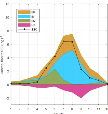
annual relative contribution equal to almost 40 %, followed by ER and SM contributing on average respectively 34 and 26 % of SSCt. Figure 6 shows the mean monthly

contribu-tion to SSCt of ER, IM, and SM averaged over the

observa-tions period. As expected, while IM contributes to SSCt

es-pecially during summer months (July–September), the frac-tion of SSCt carried by SM is higher in spring during the

snowmelt season (April–June). The effect of erosive rainfall is more evenly distributed throughout the year, and intensi-fied in summer (July–August) when the fraction of the catch-ment free from snow is at its maximum and rain intensities are high.

4.2 Long-term changes in SSC

We simulate the HMRC and the traditional RC over the 40-year period 1975–2015 at a daily resolution and compare the two simulations with observations over the same period. We sample only SSC values on days when real twice-a-week observations were taken, to make a fair comparison with observed values which exhibited a jump in 1987. A two-sample two-sidedt test for equality of the mean around this point does reveal a statistically significant jump (5 % signifi-cance level) only in mean annual SSC values simulated with HMRC and not with RC, if the actual time of the change is known a priori. Also, if we assume that the time of change is not exactly known, and we compute the probability dis-tribution functions of SSC in two separated periods before and after the observed rise in SSC (namely 1975–1990 and 2000–2015), we conclude that the observations show differ-ent distributions in the two periods (Fig. 7a) and that only the HMRC simulation reproduce similar distributions (Fig. 7b) but not the traditional RC (Fig. 7c).

Figure 5.Mean monthly values of discharge measured at the outlet

of the catchment (dash–dot grey line), SSCt derived from

observa-tions of NTU (solid blue line with circles), SSCt simulated with

the traditional RC (solid red line), and with the HMRC (solid black line with dots). Coloured shaded areas represent the range

corre-sponding to±standard error. Mean values and standard errors are

computed over the entire observation period.

5 Discussion

The robustness of the hydroclimatic predictors of SSC in this work depends on the hypothesis that the hydroclimatic vari-ables are independent drivers which activate different sedi-ment sources in Alpine catchsedi-ments. Indeed the high fraction of the daily SSCt variance explained by the first three

hy-droclimatic variables selected by the IIS algorithm, ERt−1,

IMt−1, and SMt−1, is in accordance with the physical

dynam-Figure 6. Mean monthly values of SSCt computed with HMRC

(black line with circles). Coloured areas represent the mean monthly

contribution to SSCt of ERt−1, IMt−1, SMt−1, and HPt(dilution)

averaged over the observation period.

ics in such environments. The higher intensity that character-izes rainfall events in comparison to the melting components is more likely to generate peaks of SSC during heavy rainfall and floods. In accordance, ER is responsible for a large frac-tion of the process variability (75 %). Indeed, intense rainfall events can detach and mobilize large amounts of sediment (Wischmeier, 1959; Wischmeier and Smith, 1978; Meus-burger et al., 2012). The sharp rise in streamflow, which typ-ically follows a precipitation event, results in an increase in sediment transport capacity that may further entrain sediment previously stored along channels. Precipitation is also one of the main triggering factors of mass wasting events, like landslides and debris flow (e.g. Caine, 1980; Dhakal and Si-dle, 2004; Guzzetti et al., 2008; Leonarduzzi et al., 2017), in which large quantities of sediment may be instantly released to the river network (e.g. Korup et al., 2004; Bennet et al., 2012). Conversely, the physical processes of ice melt-driven erosion and sediment transport are more gradual and contin-uous. Similarly, the slow and continuous effect of snowmelt-driven runoff on hillslope and channel erosion contributes to the seasonal pattern of SSC and plays a secondary role in explaining its daily variability and peaks in SSC. Inter-estingly, hydropower releases do not influence significantly the variance of SSC at the daily scale, despite the fact that the Rhône Basin is heavily regulated by hydropower reser-voirs. This is most likely related to the fact that water fluxes downstream of Alpine hydropower dams have lower con-centrations of suspended sediment compared to fluxes

enter-ing the reservoirs, due to sediment trappenter-ing in the reservoirs (Loizeau and Dominik, 2000; Anselmetti et al., 2007). This is in agreement with results of the sediment fingerprinting analysis recently performed in the catchment, which suggests the under-representation of sediments originated in the most highly regulated lithological unit (Stutenbecker et al., 2017). This is also indicated by the negative coefficient of HP, which suggests that hydropower releases dilute suspended sediment in the HMRC model and therefore leads to a reduction of SSCt compared to natural flow. It should also be noted that

the effect of hydropower reservoirs on sediment storage is grain size dependent (e.g. Anselmetti et al., 2007) and may be substantially different for coarser grains transported as bed-load. Moreover, it is necessary to consider that this analysis focuses on the effects of hydropower on daily suspended sed-iment dynamics at the basin scale, and neglects potential ef-fects at subdaily scale and localized in tributary catchments. For example, the instantaneous and intermittent flushing of sediment downstream of water diversions infrastructures, lo-cated at the most upstream headwater streams, may have sub-stantial effects locally.

We calibrate and validate a rating curve based on the droclimatic variables selected by the IIS algorithm and hy-dropower releases and a traditional rating curve based on dis-charge only. While both the HMRC and the traditional RC show similar performance in calibration, the HMRC, by tak-ing into account the physical processes which govern SSC in a more direct way, performs better in validation and simu-lates more accurately the seasonal pattern of SSC, especially in summer when melting of snow and ice are active and a large fraction of the catchment is snow-free and subject to erosion by rainfall. The traditional RC overestimates SSC in winter because it relies on streamflow only and does not ac-count for the low concentration of sediment coming from hy-dropower reservoirs.

(a) (b) (c)

HMRC RC

Observations

Figure 7.Empirical probability density functions of mean monthly SSC computed on twice-a-week samples:(a)observed,(b)simulated

with HMRC, and(c)simulated with traditional RC for two 15-year periods 1975–1990 (blue) and 2000–2015 (grey).

Figure 8.Mean annual contribution to SSC of ERt−1, IMt−1, and

SM_t−1simulated with the HMRC.

HMRC is capable of simulating the observed shift in SSC, al-though the simulation resembles more of a gradual increase than a sudden jump. The results show that a more process-based rating curve accounting for the different hydroclimatic forcing can not only separate the relative effects of the differ-ent forcings on SSC, but also explain climate-driven changes in suspended sediment dynamics, which is not possible by adopting a traditional rating curve based on discharge alone.

6 Conclusions

In this paper, we analyse how hydroclimatic factors in-fluence suspended sediment concentration in Alpine catch-ments by differentiating among the potential contributions of erosional and transport processes typical of Alpine en-vironments, driven by (1) erosive rainfall defined as liq-uid precipitation over snow-free surfaces, (2) ice melt, and (3) snowmelt. For regulated catchments, we include the po-tential effect of hydropower by considering the contribution to SSC of fluxes released from reservoirs due to hydropower operations. We obtained the hydroclimatic variables ER, SM, and IM by using a conceptual spatially distributed model of snow accumulation, snowmelt, and ice melt driven by

pre-cipitation and temperature at a daily resolution and we com-puted HP via a unique virtual reservoir which was operated on the basis of a target volume function, which is aimed at reproducing the cumulated effect of the historical operations of the several hydropower facilities. We then used the Itera-tive Input Selection algorithm to select the variables that play a significant role in predicting SSC and to quantify their rela-tive importance and predicrela-tive power in simulating observed changes in SSC in the Rhône Basin over a period of 40 years. We tested our approach on the upper Rhône Basin in Switzer-land. Our main findings can be summarized as follows.

1. The three hydroclimatic processes ER, IM, and SM are significant predictors of mean daily SSC at the outlet of the upper Rhône Basin, explaining respectively 75, 12, and 4 % of the total observed variance; hydropower re-leases do not play a significant role in defining the vari-ance of SSC, most likely because fluxes released from reservoirs are poor in sediment due to sediment trap-ping. The characteristic time lag of 1 day for the ER, IM, and SM fluxes, representing the time necessary to pro-duce sufficient runoff and to entrain and transport sedi-ment from a given location in the catchsedi-ment to the out-let, are in agreement with typical concentration times of the catchment; conversely for HP the time lag is lower than 1 day.

3. The HMRC is capable of reproducing the pattern of SSC even though it does not include discharge as an input variable. Although the HMRC and traditional discharge-based RC perform similarly in simulating ob-served SSC over the calibration period, the HMRC per-forms better than the traditional RC in validation at the daily scale, and in capturing seasonality, especially in summer when SSC are highest. This is particularly rel-evant because more than 66 % of the total suspended sediment load reaching the outlet of the upper Rhône Basin in the observation period is transported by SSC values larger than the 90th percentile.

4. With the HMRC approach we are able to reproduce changes in SSC in the past 40 years that have occurred in the catchment due to a temperature change, and we can demonstrate that the shift in SSC is most likely due to the increase in ice melt fluxes.

In summary, our approach provides an insight into how hy-droclimatic variables control SSC dynamics in Alpine catch-ments, and the results suggest that a more process- and data-informed approach in predicting suspended sediment concentrations, which accounts for sediment sources and transport processes driven by erosive rainfall, snowmelt, and ice melt, instead of only discharge, allows climate-induced changes in sediment dynamics to be analysed. Although these results are specific for the upper Rhône Basin only, the approach is general and may be employed in other Alpine catchments with pluvio-glacio-nival hydrological regimes where sufficient data are available.

Data availability. Data used in this study are available from the Swiss Federal Office for the Environment (FOEN, discharge, sus-pended sediment concentration and turbidity), the Swiss Federal Office for Topography (Swisstopo, DEM), and the Swiss Fed-eral Office of Meteorology and Climatology (MeteoSwiss, gridded datasets of temperature and precipitation). Basin-average daily val-ues of the hydroclimatic variables simulated in this analysis together with a detailed scheme of the hydropower system operating in the catchment provided by Fatichi et al. (2015) are available from the authors.

Supplement. The supplement related to this article is available online at: https://doi.org/10.5194/hess-22-3421-2018-supplement.

Author contributions. AC, DA, and PM designed the methodology. AC and DA developed the code and carried out simulations and computations. All co-authors contributed to the paper.

Competing interests. The authors declare that they have no conflict of interest.

Acknowledgements. We thank the Federal Office of the Envi-ronment (FOEN) for providing discharge, suspended sediment concentration, and turbidity data. We also thank Alessandro Grasso (FOEN) for the explanation on the SSC and turbidity measurement procedures. This research was supported by the Swiss National Science Foundation Sinergia grant 147689 (SEDFATE). Daniela Anghileri was supported by the Swiss Competence Centre on Energy – Supply of Energy (SCCER–SoE).

Edited by: Matjaz Mikos

Reviewed by: Tammo Steenhuis and one anonymous referee

References

Aas, E. and Bogen, J.: Colors of Glacier Water, Water Resour. Res., 24, 561–565, 1988.

Anselmetti, F. S., Bühler, R., Finger, D., Girardclos, S., Lancini, A., Rellstab, C., and Sturm, M.: Effects of Alpine hydropower dams on particle transport and lacustrine sedimentation, Aquat. Sci., 69, 179–198, 2007.

Bakker, M., Costa, A., Stutenbecker, L., Girardclos, S., Loizeau J.-L., Molnar P., Schlunegger, F., and Lane S. N.: Com-bined flow abstraction and climate change impacts on an aggrading Alpine river, Water Resour. Res., 54, 223–242, https://doi.org/10.1002/2017WR021775, 2018.

Bennett, G., Molnar, P., Eisenbeiss, H., and McArdell, B. W.: Ero-sional power in the Swiss Alps: characterization of slope fail-ure in the Illgraben, Earth Surf. Proc. Land., 37, 1627–1640, https://doi.org/10.1002/esp.3263, 2012.

Boulton, G. S.: Processes and patterns of glacial erosion, edited by: Coates, D. R., Glacial Geomorphology, New York State Univer-sity, 41–87, 1974.

Caine, N.: The rainfall intensity–duration control of shallow land-slides and debris flows, Geogr. Ann. A, 62, 23–27, 1980. Costa, A., Molnar, P., Stutenbecker, L., Bakker, M., Silva, T.

A., Schlunegger, F., Lane, S. N., Loizeau, J.-L., and Girardc-los, S.: Temperature signal in suspended sediment export from an Alpine catchment, Hydrol. Earth Syst. Sci., 22, 509–528, https://doi.org/10.5194/hess-22-509-2018, 2018.

Dadson, S. J., Hovius, N., Chen, H., Dade, W. B., Lin, J.-C., Hsu, M.-L., Lin, C.-W., Horng, M.-J., Chen, T.-C., Milliman, J. D., and Stark, C. P.: Earthquake–triggered increase in sediment de-livery from an active mountain belt, Geology, 32, 733–736, 2004. Dedieu, J.-P., Boos, A., Kiage, W., and Pellegrini, M.: Snow cover retrieval over Rhône and Po river basins from MODIS optical satellite data (2000–2009), Geophys. Res. Abstracts, 12, 5532, EGU General Assembly 2010, 2010.

De Girolamo, A. M., Pappagallo, G., and Lo Porto, A.: Temporal variability of suspended sediment transport and rating curves in a Mediterranean river basin: The Celone (SE Italy), Catena, 128, 135–143, https://doi.org/10.1016/j.catena.2014.09.020, 2015. Dhakal, A. S. and Sidle, R. C.: Distributed simulations of landslides

for different rainfall conditions, Hydrol. Process., 18, 757–776, 2004.

Duan, N.: Smearing estimate: a nonparametric retransformation method, J. Am. Stat. Assoc., 78, 605–610, 1983.

Fatichi, S., Rimkus, S., Burlando, P., Bordoy, R., and

cli-mate and anthropogenic changes on the hydrology

of an Alpine catchment, J. Hydrol., 525, 362–382,

https://doi.org/10.1016/j.jhydrol.2015.03.036, 2015.

Finger, D., Schmid, M., and Wüest, A.: Effects of upstream hy-dropower operation on riverine particle transport and turbid-ity in downstream lakes, Water Resour. Res., 42, W08429, https://doi.org/10.1029/2005WR004751, 2006.

Foster, G. C., Dearing, R. A., Jones, R. T., Crook, D. S., Siddle, D. J., Harvey, A. M., James, P. A., Appleby, P. G., Thompson, R., Nicholson, J., and Loizeau, J.-L: Meteorological and land use controls on past and present hydro–geomorphic processes in the pre–alpine environment: an integrated lake–catchment study at the Petit Lac d’Annecy, France, Hydrol. Process., 17, 3287– 3305, 2003.

Frei, C.: Interpolation of temperature in a mountainous region using nonlinear profiles and non–Euclidean distances, Int. J. Climatol., 34, 1585–1605, 2014.

Frei, C., Schöll, R., Fukutome, S., Schmidli, J., and Vidale, P. L.: Future change of precipitation extremes in Europe: An intercom-parison of scenarios from regional climate models, J. Geophys.

Res., 111, D06105, https://doi.org/10.1029/2005JD005965,

2006.

Gabbud, C. and Lane, S. N.: Ecosystem impacts of Alpine wa-ter intakes for hydropower: the challenge of sediment man-agement, Wiley Interdisciplinary Reviews, Water, 3, 41–61, https://doi.org/10.1002/wat2.1124, 2016.

Galelli, S. and Castelletti, A.: Tree–based iterative input variable se-lection for hydrological modeling, Water Resour. Res., 49, 4295– 4310, https://doi.org/10.1002/wrcr.20339, 2013.

Geurts, P., Ernst, D., and Wehenkel, L.: Extremely randomized trees, Mach. Learn., 63, 3–42, 2006.

Gippel, C. J.: Potential of turbidity monitoring for measuring the transport of suspended solids in streams, Hydrol. Processes, 9, 83–97, 1995.

Grasso, A., Bérod, D., and Hodel, H.: Messung und Analyse der Verteilung von Schwebstoffkonzentrationen im Querprofil von Fliessgewässern, “Wasser Energie Luft” – 104, Jahrgang, 2012, Heft 1, CH–5401 Baden, 2012.

Grønsten, H. A. and Lundekvam, H.: Prediction of surface runoff and soil loss in southeastern Norway using the WEPP Hillslope model, Soil Till. Res., 85, 186–199, 2006.

Gurnell, A., Hannah, D., and Lawler, D.: Suspended sediment yield from glacier basins, Erosion and Sediment Yield: Global and Re-gional Perspectives, Proceedings of the Exeter Symposium, July 1996, IAHS Publ. no. 236, 1996.

Guzzetti, F., Peruccacci, S., Rossi, M., and Stark, C. P.: The rainfall intensity–duration control of shallow landslides and debris flows: an update, Landslides, 5, 3–17, 2008.

Hock, R.: Temperature index melt modelling in mountain areas, J. Hydrol., 282, 104–115, 2003.

Holliday, C. P., Rasmussen, T. C., and Miller, W. P.: Establishing the relationship between turbidity and total suspended sediment concentration, Georgia Water Resources Conference, Athens, GA: Georgia Water Science Center Publications, 2003. Horowitz, A. J.: A quarter century of declining suspended sediment

fluxes in the Mississippi River and the effect of the 1993 flood, Hydrol. Process., 24, 13–34, 2010.

Hu, B., Wang, H., Yang, Z., and Sun, X.: Temporal and spatial varia-tions of sediment rating curves in the Changjiang (Yangtze River) basin and their implications, Quatern. Int., 230, 34–43, 2011. Huang, M. Y.-F. and Montgomery, D. R.: Altered regional sediment

transport regime after a large typhoon, southern, Taiwan, Geol-ogy, 41, 1223–1226, 2013.

Huggel, C., Clague, J. J., and Korup, O.: Is climate change respon-sible for changing landslide activity in high mountains?, Earth Surf. Proc. Land., 37, 77–91, 2012.

Konz, N., Prasuhn, V., and Alewell, C.: On the measurement of alpine soil erosion, Catena, 91, 63–71, 2012.

Korup, O., McSaveney, M. J., and Davies, T. R. H.: Sediment gener-ation and delivery from large historic landslides in the Southern Alps, New Zealand, Geomorphology, 61, 189–207, 2004. Lacour, C., Joannis, C., and Chebbo, G.: Assessment of annual

pol-lutant loads in combined sewers from continuous turbidity mea-surements: sensitivity to calibration data, Water Res., 43, 2179– 2190, 2009.

Lawler, D. M. and Dolan, M.: Temporal variability of suspended sediment flux from a subarctic glacial river, southern Iceland, Erosion and Sediment Transport Monitoring Programmes in River Basins, Proceedings of the Oslo Symposium, August 1992, IAHS Publ. no. 210, 1992.

Leonarduzzi, E., Molnar, P., and McArdell, B. W.: Predictive per-formance of rainfall thresholds for shallow landslides in Switzer-land from gridded daily data, Water Resour. Res.,53, 6612–6625, https://doi.org/10.1002/2017WR021044, 2017.

Lewis, J.: Turbidity–controlled suspended sediment sampling for runoff-event load estimation, Water Resour. Res., 32, 2299– 2310, 1996.

Loizeau, J.-L. and Dominik, J.: Evolution of the Upper Rhone River discharge and suspended sediment load during the last 80 years and some implications for Lake Geneva, Aquat. Sci., 62, 54–67, 2000.

Loizeau, J.-L., Dominik J., Luzzi, T., and Vernet J.-P.: Sediment Core Correlation and Mapping of Sediment Accumulation Rates in Lake Geneva (Switzerland, France) Using Volume Magnetic Susceptibility, J. Great Lakes Res., 23, 391–402, 1997.

Métadier, M. and Bertrand-Krajewski, J.-L.: The use of long– term on–line turbidity measurements for the calculation of ur-ban stormwater pollutant concentrations, loads, pollutographs and intra–event fluxes, Water Res., 46, 6836–6856, 2012. Meusburger, K., Steel, A., Panagos, P., Montanarella, L., and

Alewell, C.: Spatial and temporal variability of rainfall erosiv-ity factor for Switzerland, Hydrol. Earth Syst. Sci., 16, 167–177, https://doi.org/10.5194/hess-16-167-2012, 2012.

Micheletti, N. and Lane, S. N.: Water yield and sediment ex-port in small, partially glacierized Alpine watersheds in a 25 warming climate, Water Resour. Res., 52, 4924–4943, https://doi.org/10.1002/2016WR018774, 2016.

Ollesch, G., Kistner, I., Meissner, R., and Lindenschmidt, K.-E.: Modelling of snowmelt erosion and sediment yield in a small low-mountain catchment in Germany, Catena, 68, 161– 176, 2006.

Pavanelli, D. and Pagliarani, A.: Monitoring water flow, turbid-ity and suspended sediment load, from an Apennine catchment basin, Italy, Biosyst. Eng., 83, 463–468, 2002.

Stutenbecker, L., Costa, A., and Schlunegger, F.: Lithologi-cal control on the landscape form of the upper Rhone Basin, Central Swiss Alps, Earth Surf. Dynam., 4, 253–272 https://doi.org/10.5194/esurf-4-253-2016, 2016.

Stutenbecker, L., Delunel, R., Schlunegger, F., Silva, T. A., Šegvi´c, B., Girardclos, S., Bakker M., Costa, A., Lane, S. N., Loizeau, J.-L., Molnar, P., Akar, N., and Christl, M.: Reduced sediment supply in a fast eroding landscape? A multi-proxy sediment bud-get of the upper Rhône basin, Central Alps, Sediment. Geol., https://doi.org/10.1016/j.sedgeo.2017.12.013, in press, 2017. Syvitski, J. P. M., Morehead, M. D., Bahr, D. B., and Mulder, T.:

Es-timating fluvial sediment transport: the rating parameters, Water Resour. Res., 36, 2747–2760, 2000.

Syvitski, J. P. M., Vörösmarty, C. J., Kettner, A. J., and Green, P.: Impact of Humans on the Flux of Terrestrial Sed-iment to the Global Coastal Ocean, Science, 308, 376–380, https://doi.org/10.1126/science.1109454, 2005.

Van Dijk, A. I. J. M., Bruijnzeel, L. A., and Rosewell, C. J.: Rain-fall intensity–kinetic energy relationship: A critical literature ap-praisal, J. Hydrol., 261, 1–23, 2002.

Vörösmarty, C. J., Meybeck, M., Fekete, B., Sharma, K., Green, P., and Syvitski, J. P. M.: Anthropogenic sediment retention: ma-jor global impact from registered river impoundments, Global Planet. Change 39, 169–190, 2003.

Warrick, J. A.: Trend analyses with river sediment rating curves, Hydrol. Process., 29, 936–949, 2015.

Wischmeier, W. H.: Rainfall erosion index for universal soil loss equation, Soil Sci. Soc. Am. Pro., 23, 246–249, 1959.

Wischmeier, W. H. and Smith, D. D.: Predicting Rainfall Erosion Losses – A Guide to Conservation Planning, Agric. Handbook, No. 537, Washington D.C., 58, 1978.