Large Eddy Simulation of Planar Free Jet Flow Using the Space Time Conservation Element/Solution Element Scheme

2018 International Conference on Physics, Computing and Mathematical Modeling (PCMM 2018) ISBN: 978-1-60595-549-0

Large Eddy Simulation of Planar Free Jet Flow Using the Space-Time

Conservation Element/Solution Element Scheme

Ze-tian REN

, Horus Y.H. CHAN

, Randolph C.K. LEUNG

, Su-hui LI

and Min ZHU

1

Department of Energy and Power Engineering, Tsinghua University, Beijing 100084, China

2

Department of Mechanical Engineering, the Hong Kong Polytechnic University, Hong Kong, China

*

Corresponding author

Keywords: Large eddy simulation, Space-time CE/SE scheme, Planar free jet flow, Region of constant height.

Abstract. In order to investigate the characteristics of planar free jet flows, the Monotonically Integrated Large Eddy Simulation (MILES) method with the high-resolution space-time conservation element/solution element (CE/SE) scheme was used to simulate the two-dimensional free jet flows. For free jet flows within the Reynolds number range 35300~2200, the flow structures, averaged and instant velocity, turbulence intensity, velocity profiles of different cross-sections were examined respectively. The simulation results agree well with the experiment data. A region of constant height exists right after the jet outlet, in which the average centerline velocity and turbulence intensity maintains same with the jet outlet, and the instant fluctuation amplitudes are also small. For turbulent flows, the length of the undisturbed region is equal to the length of region of constant height. While near the laminar region, the length of undisturbed region is slightly larger than the length of zone of constant height. The vortex structures start to generate after the undisturbed region, develop coherently in the region of flow establishment, and break down gradually in the region of fully established flow region. As the Reynolds number increases, the length of zone of constant height, the length of undisturbed region and the length of potential core region all decrease correspondingly.

Introduction

Jet flow is widely used in aerospace, hydraulic engineering and industrial manufacturing, and the two-dimensional planar free jet flow is important for blade impingement cooling, thrust vector control and material cutting[1]. Studies have been focused on the flow structures of the planar free jet flows.

Albertson et al.[2] firstly proposed the flow evolution of a jet, emerging from a two-dimensional rectangular slot without converging duct. They reported that the flow field includes the zone of flow establishment and the zone of established flow, divided by the length of potential core region Lp. Gori

et al.[3] measured the flow structure of two-dimensional free jet at Re = 11300 by means of Hot Wire Anemometer (HWA) and shadowgraph visualizations. They reported that the region of undisturbed flow where velocity and turbulence remain almost equal to those measured on the exit. This length of this undisturbed region LU is almost equal to the length region of constant height, LCH. They further

measured the flow field of the jet flow with Re = 22000~35300 by Particle Image Velocimetry (PIV) technique[4], reported that the lengths of LCH, LU and Lp decrease as the Re number increases.

and grid adaptability, which has been successfully used in computational aeroacoustics[8] and induct turbulent flow simulation[9]. The numerical work in this study will be validated with experimental results by Gori et al.[4]

Computational Methods

Governing Equations

The problem is governed by the two-dimensional Navier–Stokes (N-S) equations together with the equation of state for calorically perfect gas, and the equations are nondimensionalized. The N-S equations without source can be written in the strong conservation form as

ˆ ˆ ˆ ˆ

ˆ _{( ) ( )}

0,

ˆ ˆ ˆ

   

 _{  }

  

v v

t x y

F F G G

U

(1)

where “^” denotes non-dimensional variables, and

ˆ ˆ ˆ ˆ ˆ ˆ ˆ ˆ       _{ }       ρ ρu ρv ρE U , 2 ˆ ˆ ˆ ˆ ˆ ˆ

ˆ ˆ ˆ ˆ ˆ ˆ ˆ

( )    _    _{ }        ρu ρu p ρuv ρE p u F

,

2

ˆ ˆ ˆ ˆ ˆ ˆ

ˆ ˆ ˆ ˆ ˆ ˆ ˆ

( )       _{ }         ρv ρuv ρv p ρE p v G , 0 ˆ 1 ˆ ˆ Re ˆ              xx v xy x τ τ α F , 0 ˆ 1 ˆ ˆ Re ˆ                xy v yy y τ τ α G

. (2) The ˆρ, uˆ, vˆ are respectively the density and velocities on x, y directions. Also, total energy

2 2

ˆ _{ ˆ / [ (ˆ 1)] ( ˆ  ˆ ) / 2}

E p ρ γ u v , pressure pˆ ρT γˆ / Mˆ 2 , αˆxτ u τ v qˆxxˆˆxyˆ ˆ x , αˆy τ u τ v qˆxyˆˆyyˆ ˆ y ,

stresses τˆ_xy      μ uˆ( ˆ/ yˆ vˆ/ xˆ), τˆ_xx 2 (2μˆ     uˆ/ xˆ vˆ/ yˆ) / 3, τˆ_yy 2 (2μˆ     vˆ/ yˆ uˆ/ xˆ) / 3, heat

fluxes qˆ_x  [ / (μ γˆ 1) PrM ]2 Tˆ/xˆ, qˆ_y  [ / (μ γˆ 1) PrM ]2 Tˆ/yˆ. The specific heat ratio γ1.4,

non-dimensional numbers are Reynolds number Re ρ u L μ_{0 0 0} / ₀, Mach number Mu₀/c₀, Prandtl

number Prc_p,0μ λ₀/ ₀ 0.71.

Numerical Schemes

The space-time conservation element/solution element (CE/SE) implicit numerical scheme is used in this study. This scheme retains the conservation feature in both space and time domains through the proper construction of the conservation element and solution element. Also, the two-dimensional problem can be treated as three-dimensional by unifying the space and time domains E3  X( , , )x y t .

According to the Gauss's divergence theorem, Eq. 1 can be written into integral form

( )  0,



(3) where K X( )[ ( ), ( ), ( )]F X G X U X , S(V) is the surface of the space-time region, ds(dx dy dt, , ) is the normal vector on the surface, and Kds is the flux through the surface S(V).

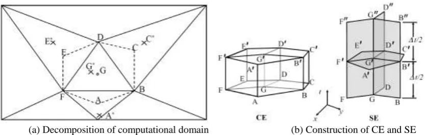
Fig. 1 describes the mesh and the construction of the conservation element and solution element. In the two-dimensional triangular mesh in Fig. 1(a), G* is the centroid of ABCDEF, where the calculated flow variables will be stored. G* is thus called “solution point”. The time interval in Fig. 1(b) is 1/2 of

the numerical time step, and the hexahedra ABGFA’B’G’F’, BCDGB’C’D’G’ and DEFGD’E’F’G’

are the three space-time conservation elements, CEs. The four planes BGG’’B’’, DGG’’D’’,

(a) Decomposition of computational domain (b) Construction of CE and SE

Figure 1. Geometrical definitions of conservation element and solution element.

As the CE/SE scheme has the advantages of global conservation, monotonicity, positivity and locality, the Monotonically Integrated Large Eddy Simulation (MILES)[7] is used in this study, in which the numerical dissipation is used to mimic the turbulent dissipation without use of SGS models. The high resolution of MILES has been verified to be satisfied to simulate jet flows[10].

Results

In this study, the planar air jet flow is simulated under various Reynolds numbers. The computational domain is rectangular and -15<x/H<10, -3.5<y/H<3.5, where H is the width of the free jet. Uniform inflow condition at x/H = -15, non-slip condition at side walls, and free outlet conditions at other boundaries are used. The total grid number is 1092400, and the regions near the jet outlet and boundaries are refined. For different Re numbers, the velocity distribution, vorticity field, and turbulence intensity are analyzed. The time-averaged centerline turbulent intensity is calculated by

2

, ₁ 0

0

1 1

( ) [%], 





u N _j j

T u u

u N ₍₄₎

where u0 is the time averaged stream wise velocity on the centerline at the jet outlet. The turbulent

intensity at the jth instant Tu,j can also be obtained by

,   0 / 0 [%].

u j j

T u u u

(5) Fig. 2 shows the results for Re = 2200, the upper laminar case. It can be seen that the width of the free jet remains unchanged for a long distance after the jet outlet, defined as the length of region of constant height LCH, which is about 4.5H in this case. The two shear layers and the cross-section velocity profile remains steady before x = 6.0H, which is called the length of undisturbed region LU. The time averaged centerline velocity and turbulent intensity both remain unchanged in the region of constant height, shown in Fig. 2(c) and Fig. 2(d). The amplitudes of instant centerline velocity and turbulent intensity within the region of constant height are very small (<3%), while increase distinctly after LCH. The length of potential core region LP is defined as the distance where the time averaged centerline velocity decreases to 95% of u0, and LP is 7.5H in this case.

When the Re number is increased to 35300, the turbulent flow shows different features. It can be seen from Fig. 3(a) that the width of the free jet remains unchanged for a very short distance after the jet outlet, and the length of region of constant height LCH is about 1.2H in this case. The length of undisturbed region LU is nearly the same as LCH, in which the shear layer and velocity profile remain

undisturbed. The amplitudes of instant centerline velocity and turbulent intensity within the region of constant height are very small (<3%). The length of potential core region LP also decreased to about 5.0H in this case, after which the unsteady vortex structures begin to break down.

Figure 2. Results for Re = 2200, (a) Time-averaged u velocity contour, (b) Instant vorticity field, (c) Time-averaged and instant centerline u velocity, (d) Time-averaged and instant centerlineturbulence intensity.

Figure 3. Results for Re = 35300, (a) Time-averaged u velocity contour, (b) Instant vorticity field, (c) Time-averaged and instant centerline u velocity, (d) Time-averaged and instant centerlineturbulence intensity.

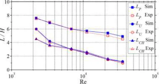
potential core region LP are compared with the experiment results[4], as shown in Fig. 4. It can be seen that LU is nearly the same with LCH for turbulent cases, but is slightly larger than LCH in the upper laminar region. The characteristic lengths decreases as the Re number increases, and the simulation results agree very well with the experiment.

Summary

In this study, the two-dimensional free jet flows are simulated using the MILES method combined with space-time CE/SE scheme. The simulated velocity and turbulence intensity distributions are compared with the experiment results.

constant height LCHdecreases from 1.2H for Re = 2200 to 4.5H for Re = 35300. The length of potential core region LP also decreases from 5.0H for Re = 2200 to 7.5H for Re = 35300. The unsteady

vortex structure movement starts after the length of undisturbed region LU, develop coherently in the region of flow establishment and break down gradually after the length of potential core region LP.

Figure 4. Comparison of lengths with different Re numbers.

Acknowledgement

This research was supported by the Joint Supervision Scheme of PolyU, the National Natural Science Foundation of China (No. 51676110) and Tsinghua National Laboratory for Information Science and Technology.

References

[1]H. Kashimura, Y. Masuda, Y. Miyazato, and K. Matsuo, Numerical analysis of turbulent sonic jets from two-dimensional convergent nozzles, J. Therm. Sci. 20 (2011) 133-138.

[2]M.L. Albertson, Y. Dai, R.A. Jensen, and H. Rouse, Diffusion of submerged jets, ASCE Paper. 74 (1948) 1571-1596.

[3]F. Gori, F. De. Nigris, and E. Nino, Fluid dynamics measurements and optical visualization of the evolution of a submerged slot jet of air, 12th Int. Heat Trans. Conf. 2 (2002) 303-308.

[4]F. Gori, I. Petracci, and M. Angelino. Flow evolution of a turbulent submerged two-dimensional rectangular free jet of air. Average Particle Image Velocimetry (PIV) visualizations and measurements, Int. J. Heat Fluid Fl. ,44 (2013) 764-775.

[5]C. Le. Ribault, S. Sarkar, and S. Stanley, Large eddy simulation of a plane jet, Phys. Fluids. 11 (1999) 3069-3083.

[6]S.C. Chang, The method of space-time conservation element and solution element-a new approach for solving the Navier-Stokes and Euler equations, J. Comput. Phys. 119 (1995) 295-324.

[7]J. Boris, F. Grinstein, E. Oran, and R. Kolbe, New insights into large eddy simulation, Fluid Dyn. Res. 10 (1992) 199-228.

[8]C.Y. Loh, L.S. Hultgren, Jet screech noise computation, AIAA J. 44 (2006) 992-998.

[9]G. Lam, R. Leung, and S. Tang, Aeroacoustics of duct junction flows merging at different angles, J. Sound Vib. 333 (2014) 4187-4202.