When is There a Representative Consumer of Public Goods? On Separating the Allocation and Distribution Branches of Government

Research Seminar in Quantitative Economics

Discussion Paper

m -

--DEPARTMENT OF ECONOMICS

University of Michigan

ALLOCATION AND DISTRIBUTI ON BRANCHES OF GOVERNMENT

C-38

THEODORE C. BERGSTROM UNIVERSITY OF MICHIGAN

AND

AUSTRALIAN NATIONAL UNIVERSITY

AND

RICHARD C. CORNES

AUSTRALIAN NATIONAL UNIVERSITY

June 1981

If all the trees were one tree, What a gteat tree that would be!

And if all the axes were one axe, What aaest axe that would be!

And if all the men were one man, What a gPCeat man that would be!

And if the gAezas man took the geca axe,

And cut down the ctCCt tree,

And let it fall into the age.at sea, What a splish-splash that would be!

Normally aggregate demand for private goods can not be treated as if it were the demand of a single gigantic rational consumer. This is possible only if "income distribution doesn't affect aggregate demand". Gorman (1953) dis-covered restrictions on the form of indirect utility functions that are

necessary and sufficient to allow such aggregation. In early partial equili-brium treatments of public goods theory by Lindahl

C1910)

and Bowen (1943) the efficient amount of public goods- appears to be determined independently of

income distribution. Samuelson (1955), (1966) observes that generally an efficient amount of public goods cannot be determined independently of the

distribution of private goods. He points out that such separation is possible in the special case where preferences of all consumers are quA--Zinea t, that is, representable by utility functions that are linear in private goods.

Mus-grave (1966) responds that although independence of allocation from distribu-tion is not legitimate in a strict logical sense, separation of allocational decisions from distributional decisions is a useful simplification of reality that may in practical situations lead to better decision making than attempts

to simultaneously determine allocation and distribution.

If quasi-linear preferences were necessary for separation of allocation from distribution, then Musgrave 's case for separation, even as an

re-futable implications. For example, it implies a zero income elasticity of demand for public goods. Several recent studies of the demand for public goods strongly rej ect the hypothesis that the income elasticity of demand

for local public goods is close to zero. As it turns out, however,

separa-tion of allocation from distribution is possible for a much broader class of

preferences. This class is essentially dual to the class of preferences found by Gorman to admit construction of a "representative consumer" in the

theory of demand for private goods. 2

In the next section we develop a rigorous theory of when allocation can be separated from income distribution, or equivalently of when there is a repre-sentative consumer of public goods. It remains an open question whether

empirical data can be found that refute the hypothesis that preferences for public goods allow such aggregation. This being the case, it also remains to be decided whether the assumption that pref er

ences

satisfy this hypothesis yields misleading guidance for public policy.

rn the final section of this paper we show that the assumption that

pre:erences belong to the class that allows a representative consumer has

interesting implications for the theory of social welfare functions, for Lindahl's allocation theory, and for Bowen's majority voting theory. We also demonstrate that demand revealing mechanisms of the kind introduced by Clarke (1971) and

Groves and Loeb (1975) for the case of Quasi-linear utility can be extended

in a simple way to this much broader class of preferences.

SECTION 1

A. Two heuristic claims and their imrlications

Claim S - If all consumers have utility functions of the functional form A(Y) X +

,Bi(Y)

, then the =Pareto efficient quantity of public goods is in-,dtpe ndent of .the .distrihution f -pr.vate goods,

Claim -N .- If the Pareto efficient ;quantity of :public goods Is ,independent of the distribution of private goods., then all -consumers have iutti-ity func-tions of the form ACY)X + B.(Y1.

i 1

In these claims there is some good news and some bad news. The good news is Claim S. The class of preferences that allow separation of allocation from distribution is much larger than the quasi-linear family. The special

case where A(Y) = 1 is the quasi-linear case. If A(Y) -a for a > 0 and

B (Y) -= 0, pr.ef er enc es

are

identical and Cobb-Douglas. But A(~Y) .and B .(Y )

j 1.

could he chosen so that preferences are neither homothetic, separable, or identical. The bad news is found in Claim N. This -r-esult states restrictions on the class of preferences which admit separation between allocation .and distribution. Some of the implications of membership in this class are stated

in

Theorem1..

Theorem 1

Let preferences of consumer i be represented by a differentiable utility

function A(Y)X + B i(Y) where A(Y) > 0 for all Y > 0.

(a) Preferences of consumer i are homothetic if and only A(Y) is homogeneous of some degree a and B.(Y) is either constant or homogeneous of degree

a

+ 1. If there is only one public good, A(Y)X4 + B (Y) = Y X + kT ~l for some k4.

(b) Pr efer enc es o f c onsumer i ar e ad dit ively s eparable between public

and private -goods if and only if they are representable by a

utility function of the form A(Y) (X.+ k.) for some kI.

(c) Preferences of each consumer i are additively separable and

homothetic if and only if all consumers have identical

pre-ferences representable by utility functions of the form A(Y)X

where A(Y) is a homogeneous function.

If

there is only one public good, this implies that utility functions all have the Cobb-Douglas

form YaX. for some

a

> 0.

The assumptions that A(Y)X. + B (Y) and A(Y)X. + I (Y) are quasi-concave

2 i _2i

will play an important part in the development of our theory. It is therefore useful to identify some necessary and some sufficient conditions for

quasi-concavity of these functions.

Theorem 2

B (Y)

Define the function S.(Y) = . Then A(Y)X +B.(Y) EA(Y)(X.+.(Y)).

2. (Y i 2 1 2i

The following conditions are each sufficient for A(Y)X. + B .(Y) to be quasi-concave.

(i) A(Y) > 0 and £.(Y) > 0 for all Y > 0 and the functions

A(Y) and (Y) are concave.

(ii) There is only one public good, A(Y) > 0 and B(Y) > 0 for all Y > 0 and the functions A(Y) and B (Y) have non-negative first derivatives and non-negative second derivatives.

2 2 T

(iii) The two quadratic forms, V A(Y) - 7A(Y) VA(Y) and

v

(Y)f[V2A(Y) - -~ VA(Y)VA(Y)1 + A(Y) 7V ,(Y) are both

A(Y)

negative semi-defrinite and one of them is negative d

e-finite for all Y > 0.

The following conditions are each necessary for A(Y)X.+B.(Y) to be aasi-concave.

2. 1

(i) A(Y) and B()are both quasi-concave functions.

Thge coedit ion on quiadatic

f orms

is seen to be (essentially) a nec essary

and snff iciest condition for quasi-conicavity . However,. ia general thiis.

con-iton

Is,

rathex dif ic.1t to verify or

to

interpret.. Siificient conditions (i) and

C(LL)

are easier to interpret buzt are not neceessary conditions... In our appl~ications, hover, they- ii.

serve adequ~at ely.

An easy consequ

en

a of theorem 2 is

the

f oLlo d±ng.

Corollary 1J - If all individual utility functions satisfy- necessary condition

(±) or (Li) , of tiheorem 2 then the fnnc tLion ACT) I -4:L

(T)

is atas i-concave.

B. Establ~isbhing Clam S - Suafficiencv

Define an outcome to be a vector (X1,... , T,) where

Xi

is the amount of private good for i and Y is the Ca-dimensional) vector of public goods..

Let the set

of

feasible outcomaes be t((X,...., X ,)

,~Y) c-F} for some set

F

C Rel. An interior outcome is an outcome

such

that. I. > 0 for- all L. An

interior Pareto ovtimta is a Pareto optimal interior outcome.

If all consuimers

have

utilty functions of the form A(Y).X 4+ B , (), a

possible nandate for the allocation branch is: "Choose (K,Y) to narimize +

() = ()

C

on the set F ".

We

show that an allocation branch that follows

it

this instruction will choose

an

aggregate output Level that yields a Pareto

optimal outcome no natter how the private good is divided. Furthermore, given convexity, all of the "interesting" Pareto ovtima are found in this way.

--It is instructive to consider the application of Theorem 3 to a special case.

Example 1. There are two consumers with identical quasi-linear utility functions X + /Y. The set of feasible aggregate outputs

is F = {(x,Y) > OIX + Y = 3}.

In this example A(Y)X + EB.(Y) is maximized on F at X = 2, Y = 1. According to ii

Theorem 3, all outcomes that have one unit of public good and some distribution of two units of private good between the consumers are Pareto optimal. Since the convexity conditions of theorem 3 apply, it must also be that all interior Pareto optima have exactly one unit of public good and two units of private

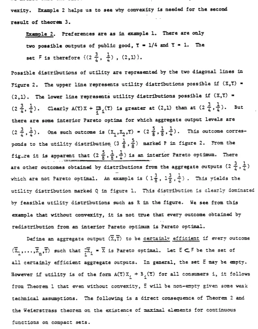
goods. There are also some non-interior Pareto optima for which Y # 1. In fact, an outcome is Pareto optimal if 1 < Y < 2 and one of the consumers gets

no private goods while the other gets 3 - Y. The utility possibility frontier

for example 1 is shown in figure 1. Points on the line between (1,3) and (3,1) correspond to outcomes where Y = 1. Points on the curved lines from (3,1) to

1 1 1 1

(3 , 2 ) and from (1,3) to ( , 3 1) represent non-interior Pareto optima. In theorem 3, although we assumed preferences to be monotone increasing in

private goods, no assumption was made about monotonicity in public

goods. This is fortunate, since to model externalities in a natural way we

need some public goods that are desirable to some consumers and undesirable, at

least in certain cuantities, to others.

Theorem

2 and its corollary specify

an interesting class of functions for which our assumption that utility is

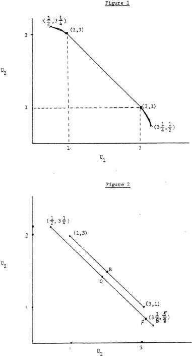
We notice that the first statement of Theorem 3 is true independent of con-vexity. Example 2 helps us to see why convexity is needed for the second result of theorem 3.

Example 2. Preferences are as in example 1. There are only

two possible outputs of public good, Y - 1/4 and Y 1. The 3 1

set F is therefore {(2 , ) , (2,1)).

Possible distributions of utility are represented by the two diagonal lines in Figure 2. The upper line represents utility distributions possible if (X,Y) (2,1). The lower line represents utility distributions possible if (X,Y)

(2 ,

$).

Clearly A(Y) X + (Y) is greater at (2,1) than at (2 ,). But there are some interior Pareto optima for which aggregate output levels are

(2 -, 4) . One such outcome is (xX 2,Y) - (2 , I, Z). This outcome

corres-1)5

ponds to the utility distribution (3 ,) marked P in figure 2. From the fig-re it is apparent that (2 5, 1,1) is an interior Pareto optimum. There

3 1 are other outcomes obtained by distributions from the aggregate outputs (2 ,4

3 31i

which are not Pareto optimal . An example is (1-s, l ) . This yields the

utility distribution marked Q in figure 1. This distribution is clearly dominated by feasible utility distributions such as R in the figure. We see from this

example that without convexity, it is not true that every outcome obtained by redistribution from an interior Pareto optimum is Pareto optimal.

Define an aggregate output (X,Y) to be certainly efficient if every outcome

(L ,...,X ,Y) such that

:X

-i=Xis Pareto optimal. Let E C. Fbe the set of all certainly efficient aggregate outputs. In general, the set E may be empty.

However if utility is of the form A(Y)X. + B.(Y) for all consumers i, it follows

:rom Theorem 1 that even without convexity,

E

will be non-empty given some weak technical assumptions. The following is a direct consequence of Theorem 2 and the Weierstrass theorem on the existence of maximal elements for continuous functions on compact sets. [image:12.631.57.567.96.746.2]

utility functions of the form A(Y)X₁ +

B

(Y) and if F is closed and bounded,

then the set E of certainly efficient aggregate outputs is non-empty.

According to theorem 3, every aggregate output (X,Y) that maximizes A(Y)X + B.(Y) on F belongs to the set E of certainly efficient aggregate outputs. In general, however, E is larger than the set of maximizers of A(Y) X + 2Bi(Y) on F. To see this, consider the following example.

i2

Example 3. There are two consumers. Consumer i has a utility

function of the form A(Y)X + B.(Y) where A(Y) = 1 for all Y and i 2.

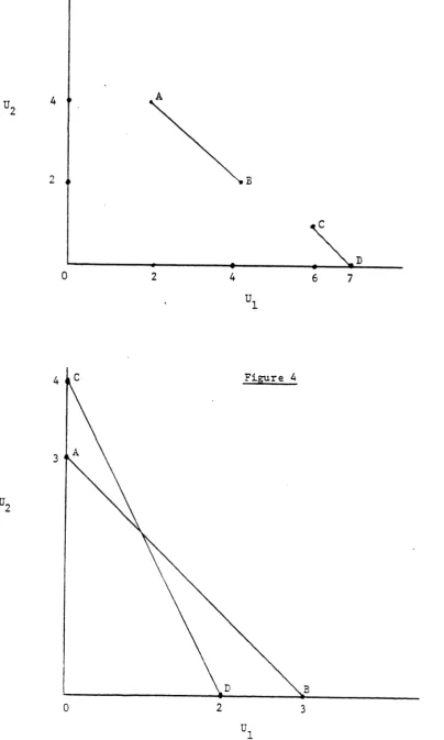
where B1(0) = B2(0) = 2, B3(1) = 6 and B2(1) = 0. Let F = {(1,1),(2,0) }.

The utility possibility frontier is described in figure 3. Utility dis-tributions obtainable when Y = 0 are represented on the line AR. Utility

distributions obtainable when Y = 1 are represented on the line CD. All of these distributions can be seen to be Pareto optimal. Therefore the set E

contains both of the points (1,1) and (2,0) from F. However if (X,Y) = (2,0), then A(Y) X + ZB .(Y) = 6 and if (X,Y) = (1,1) , A(Y) X + ZB.(Y) = 7. Therefore

ii i1

the set C is larger than the set of maximizers of A(Y) X + EB, (Y) .

It is of interest to find a binary relation whose maximal elents on P

constitute precisely the set E. As it turns out, characterizing this result is also the key to our converse result, claim N. Let us define a binary rela-tion (Q over aggregate outputs so that (X,Y) a (X',Y') if some'outcome obtained by distributing X is Pareto superior to some outcome obtained by distributing

X'. More formally, (X,Y)

0

(X',Y') if and only if there exist outcomes

(X,... ,X ,Y) and (X ,..X',Y') such that X. = X, EX = X' and

(x

X , Y),X is areo speror o( ,...X Y'). From the definitions, it is easy to verify the following.

Remark 1 - _{For arbitrary preferences, the set E of certainly eff icient aggregate}

In general, the binary relation Q may have cycles and therefore may not have a maximal element even on a finite set F. One such case is illustrated in'example 4.

Example 4. There are two consumers. Let U1(X1,Y) = X for all

Y and U2(2,) X₂ and U₂(x₂,1) = 2X2. Let F = {(2,1),(3,0)}.

The functions U (-) andtU2(-) are not of the special form A(Y)X + B (Y).

Utility distributions possible when aggregate output is (3,0) are represented by the line AB in figure 4. Distributions possible from (2,1) are represented by CD. From figure 4 and the definition of Q it is clear that (1,1) Q (2,0) and also (2, 0) > (1,1) . Therefore 0 has a cycle (of length 2) . Clearly G

has no maximal elements on F and (equivalently) the set E is empty.

Suppose preferences of all consumers are representable by utility func-tions of the form A(Y)X. + B (Y) . Then if (X,Y) > ( X' ,Y') it must be that there exist outcomes (X,...,XY) and (X ,..,K',Y') such that IX.= X,

X!

= X'

' n1 n.'i i 'i z

and A(Y)X. + B.(Y) > A(Y')X' + B.(Y') for all i with strict inequality for some

2i 21 = 1. 21

i. Therefore if (X,Y) > (X',Y') it must be that A(Y)X + B.(Y) > A(Y')X' +

B .(Y') . From this fact, the following is obvious.

Remark 2 - If preferences of all consumers are of the form A(Y) X + TB (Y) ,

i

then the relation

0

has no cycles.

A standard theorem (see Bergstrom (1975)) is that if a continuous binary relation has no cycles, then it takes maximal elements on compact sets. This

fact, with remark 2 provides an alternative derivation of corollary 2.

It is interesting to compare the relation Q) with the more familiar Kaldor-Hicks-Samuelson partial order which was central to discussions of the "new

welfare economics" (see Chipmaan and Moore (1978)) . The K.H.S. relation is

de-f ined over aggreg ate output s as f ollows:

(X,Y)K.

R.

S.

(X'

,Y')

if and only if

Xm,Y)such that

ZX.

= X and such that (XIS,...,n,Y) is Pareto

i 2.

superior to (Xl,...,X',Y')

From the definition of the K.H.S. relation and from the fact that a continuous binary relation with no cycles takes minimal elements on compact sets, it is easily shown that:

Remark 3 - If individual preferences are symmetric and transitive, then the

relation K.H.S. has no cycles. If individual preferences are also continuous and F is compact, then the set of K.H.S. maximal elements of F is non-empty.

Define an aggregate output (X,Y) to be potentially efficient if there is some Pareto optimal outcome ()L,. .. ,XmY) such that

IX.

= X. Let E* denote

i i

the set of all potentially efficient aggregate outputs in F. From the

de-frinitions it is easy to verify the following.

Remark 4 - The set' of K.H.S. maximal elements of F is equal to the set E* of

potentially efficient aggregate outputs.

in general the set E* of potentially efficient aggregate outputs is larger

than the set E of certainly efficient aggregate outputs. Equivalently the set

of K.H.S. maximal elements on F contains the set of > maximal elements of F. For instance, in example 1 above,

E

= {(2,1) } while E* = {(X,Y)

1X+Y

= 3 and

Y 12. In example 4, E is empty, while E = F = {(2,0),(1,1)Y.

Although, as we see from remark 3, the set of K.V.S. maximal elements is never empty for "wall-behaved" preferences and compact F, this set is in general

C. Establishing Claim N - Necessity

A miimal requirement for the allocation branch to .be able to choose

efficient aggregate output independently of income distribution, is tbat the

set E of certainly efficient aggregate outputs must be non-empty. As remarked

in the previous section,

E

is -equal -to the set 0 marimal elements on F.

Suppose that the set of ( maximal elements of F is non-empty for all closed bounded sets F. Then, in particular, (D must have at least one maximal element

on all finite sets R. But this is possible if .and only if a has no cycles.

Therefore a necessary condition for independence of allocation from

distribu-tion on all closed bounded feasible -sets F is that the relation()has no cycles.

Theorem 4 states conditions under which the absence of cycles in () implies that

utility functions take the form A(Y)X. + B (Y).. This establishes our claim N.

2 i

Since we regard the proof of theorem 4 to be novel and interesting we include it in the text rather than in the appendix..

Theorem 4

Let preferences of each consumer be representable by a continuous utility

function UT(X.,Y) that is monotone increasing in .. Let there be some YO such that U.(X.,Y) > U (X.,Y°) for all Y > 0 and assume that for all I !, and Y'

i i = i i i

there exists X! such that

U.-(XI,Y

1₎

> U.(X.,Y) . If the binary relation > has no

S1 1 1 2.

cycles, then for each i, U.(Xi,Y) is a monotone transformation of a utility

func-tion of the form: A(Y)X. + B.(Y) .

proof of Theorem .4

From our as sumpvtions it f ollows that

f

or every (X,. ,) , ther e exists a unique X~ such that U.(X',Y 0) = U (X.,Y) . Therefore we can def ine U.*(K, ,Y) so that U,(U.*(X.,Y) ,Y ) = Ui(Xi,Y) represents 1's preferences. Furthermore, we see

The assumption that Qhas no cycles implies that if

EX.

= EX' = X, then

i i

EU *(X.Y) =tJ.*(X.',Y). For suppose not. Then without loss of generality,

Si i' ii

6

let ZU *(X,Y) - EU*(X ',Y) = 6 > 0. Let Z. = U.*(X ,Y) --- and let

i i j iii1

3

I 2n

Z

' = U *(X ',Y) + Then ZZ. = Z'E Z. Now U *(Z Y°) = Z < U.*(XY

i i i

)

2n i i i i i iY)

for all i and U *(Z ',Y°) = Z ' > U *(X ,Y) for all i. Therefore (X,Y) 0 (Z,Y°)

and (Z,Y°) > (X,Y) . But this contradicts the assumption that ( has no cycles. From the result of the previous paragraph it follows that 7U.*(X.,Y) =

U(Xi,Y) for some function U. An equation of this functional form is known as

i

Pexider's functional equation. It is well known (see Aczel (1966)) that Pexider's functional equation implies that U.*(X.,Y) = A(Y)X. + B (Y) for all i. Since

. 2. 1 i

Ui*(X.,Y) represents i's preferences, Theorem 4 is established.

Q.E.D.

SECTION 2 Applications

If preferences are representable by utility functions of our special form, then several of the standard problems in the theory of public finance and welfare economics have interesting special solutions.

A. Cardinal U4ili:s and Social Welfare Functions

Classical utilitarians (Edgeworth (1881)) proposed that the goal of society

should be to maximize the sum of human happiness. Since Pareto, it has been

well-known that to maximize the sum of utility functions representing individual

pre-ference is not a well-defined prescription, since such functi::E are unique only

up to monotone transformations. _{Bergson (1938) and Samuelson (1947) have suggested}

that ethical value systems which respect the Pareto ordering can generally be represented by a social welfare function which depends (not necessarily in a linear way) on the level of "utili~y" _{of each consumer according to an arbitrary,}

but prespecified, utility representation of each consumer's preferences.

Where utility functions are of the form: U,(X.,Y) =A(Y)X, + B.(Y) ,

con-.

i2i i.

sider the function W(X1,...,X ,Y) = U.(X.,Y) = A(Y) IX. + 2.(Y).

Lf the technical conditions of Theorem 3 are satisfied, then finding an interior Pareto optimum is equivalent to finding an allocation (X ,..,X,Y) that

maxi-izes W() subject to the feasibility constraint, (Xi,Y) cF. The function, W('), is therefore very useful as a guide to solving for efficient aggregate

outputs. On the other hand, it provides absolutely no guidance about distribution

of private goods. In fact all redistributions of the same amount of private goods yield the same value of W. This is as it should be since we sought condi-tions under which efficient levels of aggregate output could be chosen independently

of income distribution.

It would be misleading to think of W(') as a "social welfare function" in the sense employed by Bergson and Samuelson. Notice that W(') ascribes a higher "score" to any Pareto optimal allocation, no matter how asymmetrically private goods are distributed, than it does to any less efficient but much more symmetric distribution. Clearly then such a function could not represent the distributional preferences of a person with continuous preferences, who although he wishes all individuals to be happier, has some taste for equality.

In fact, the function W(.) defined above is not the only function that will

always pick a Pareto optimum when maximized on the feasible set. Consider the

function W(X ... X ,Y) = W(X ,...,XY) - z(X. ) where X = - 1X.. Clearly

i'm 1 m ) hi n Cle

W* gives a higher value to some non-optimal equalitarian allocations than it does to some asymetric Pareto optimal allocations. On the other hand, it is easily

seen that maximizing W* on the feasible set will always yield a Pareto optimal allocation. In fact this procedure will yield an allocation that maximizes W on the feasible set and has the additional property that X = X2 = *. =X

Of course W* is not the only "social welfare function" that reflects concern

clear, from this discussion, that the function W(-) does not typically represent

a full schedule of belief about the ethics of distribution. In fact the state-ment "Maximize W on the feasible set" has no more content than we built into it.

Under appropriate conditions this condition is equivalent to "Find aggregate output levels that can be distributed to yield interior Pareto optima". There

is no implicit recommendation about distribution.

B. Lindahl Equilibrium

A Lindahl equilibrium occurs when individual "tax prices" are adjusted in such a way that, given their tax prices, consumers agree unanimously on the amount of public goods to be provided. Lindahl equilibrium is known to be Pareto optimal and to belong to the "core" when public goods are desirable. (Foley (1970)). In case utility functions are of the special form

(1) A(Y)X. +B.(Y)

1 .

Lindahl equilibrium has a very special structure. As it turns out, in this case Lindahl tax schedules will be aff ine in wealth. This means that such taxes could be collected by means of a proportional wealh tax (at the same rate for

every-one) augmenred by a "head tax" that may be positive or negative for an individual

depending on the private functions, Bi(Y).

We conduct this discussion with a simplified formal model which could be extended in a straightforward way to more genera. environments. Let there be

one private good and one public good. Each i has an initial endowment W of

private good. Public goods can be made from private goods at constant unit cost c. The set of f easible allocations , then, is

A Lindahl equilibrium consists of tax shares t , f or each i where Et. = 1 and a feasible allocation (Xi,...,Xm'Y such that for all i, (X ,Y) maximizes UI (X.,Y)

subject to the budget constraint X. + t.cY = W1. In Lindahl equilibrium,

2 3. i

therefore, each consumer's marginal rate of substitution between public and private goods equals his tax price tic.

If utility functions are of the form (1), then marginal rates of

substitu-A'()f (Y)

B-tion take the form a(Y) X + Ti(Y) where a(Y) = and Y (Y) =

Therefore, in Lindahl equilibrium,

(2) tic = a(Y)X. + Y.(Y) = a(Y)[Wi - t.cY] + y.(Y) .

Rearranging equation (2), we have:

(3) tic= a(Y)

W.

+ Yi__ _

1 + a(Y)Y 1 + -a( Y

From (2) we see that, as promised, each consumer's tax share is an affine function of his wealth. Summing equation (2) over the its, recalling that

t. = 1, and rearranging terms, we find that:

(4) c = a(Y) [W - cY] + :y )

which is just the Samuelson first order condit ion f or efficiency applied to this case. Thus if the government knows the utility functions, it could compute

Lindahl equilibrium simply by solving equation (4) for Y and then assessing taxes t cY where tic is found from equation (3). These taxes will just pay for Y and all consumers, given their tax rates, will agree that Y is the "right" amount of public goods.

C.

Majority Voting Equilibrium

A serious disadvantage of the Lindahl allocation method is that it requires the government to know details of individual preferences which are private information and which individuals may have an incentive to conceal. A less stringent requirement would be that the government knows A(Y) and has a good estimate of

II(Y)

= B.(Y). Then the government would know an "iaverage utility

function"

(1) A(Y) X +B(y)

although it would not know detailed individual preferences. The government would know enough to find an efficient amount of public goods since it needs only to choose Y to maximize:

(2) A(Y) X + B.(Y) = A(Y) X, + nB(Y) ii ij2

subject to the feasibility constraint.

If taxes are assessed according to an "average" Lindahl schedule, we have:

(3) t c = W. +

1 + a(Y)Y .+ a(Y)Y

- A'(Y)

where a(Y) = _AIM

A(Y)

and y (Y) =.()= -= EY.(Y).

A(Y) nji 2

Suppose tax shares are set by the schedule (3) and consumers are allowed to vote

on the amount of public goods. If the amount of public goods were Y, then the

utility of consumer i after paying his taxes would be

(4) U.(Y) = A(Y)[W. - t.cY] + B (Y).

If consumer i has convex preferences, then the function U.(Y) will be cuasi-concave

in Y and hence single-peaked. Consumer i's "peak" is Y* where Y* maximizes U.(Y). Let

Y* be the median of the Y 's. Since preferences are single peaked, Y* would be the

only stable outcome of a pairwise majority voting process. By straightforward calculation we see that:

(5) U'.(Y) -. C as a(Y)[W. - t .cY) + y'.(Y) -- t.c.

i. < i. 1. i < 2

(6)

U'Y-

as y.() - y(Y).

Therefore Y* -Yas Y (Y) y(Y) i<. i <

Suppose, now, that the functions y,(-) are symmetrically distributed over the population. Then the mean, y(Y) , of the terms, y (Y), will equal their median. This fact, together, with (6) implies that just as many people will want more as willwant

less public good. Therefore Y = Y*, the median of the favorite amounts. It follows that if taxes are assessed according to (3) and if preferences are symmetrically distributed in this sense, then maj ority vote will select the Pareto efficient quantity, Y. This generalizes a result of Bowen (1943) who

showed that if preferences are symmetrically distributed and quasi-linear and if taxes are the same for everyone, then the majority rule outcome is Pareto optimal.

D. Demand-Revealing Mechanisms 5

Clarke (1971) and Groves and Loeb (1975) have demonstrated that if utility

is quasi-linear, then there exists an "incentive compatible" mechanism that

de-term2ines the supply of public goods and individual tax rates. This mechanism

uses information supplied by consumers about their own preferences and has the

property that honest revelation of preferences is a dominant strategy for each consumer. The amount of public goods selected will satisfy the Samuelson marginal rate of substitution conditions. Groves and Ledyard (1976) suggest

that in more realistic cases where the demand for public goods is income

respon-sive, it may be necessary to settle for a preference revelation mechanism in which honest revelation is a Nash equilibrium but not a dominant strategy. They concede

however , t hat Nas h equ ilibr ium in this cont ext is a les s p er suas iv e game

theoretic "solution" than dominant strategy. We show here that the Clarke, Groves-Loeb results generalize to the case where utility functions are of the

(1) U (XY) = A(Y)X. + B.(Y)

i i 1 2.

where U is strictly quasi-concave. 6

The procedure in its simplest form assumes that the function A(Y) is public information. The mechanism induces consumers to honestly reveal the "private information" B (Y), in their utility functions. Let the technology be as follows . Each consumer i has an initial endowment of private goods, W . Public good is produced from private goods at a total cost C(Y) where C'(Y) > 0 and C"(Y) > 0. The set of feasible allocations is then the convex set:

{(X ,...,X'Y) IX + C(Y) = W}. All consumers are asked to reveal their

func-1 m ii

tions B (-). Each i then reports a function N.(-) (possibly different from

i 2

B.(-)). Let M = (M (-) ,...,M (-)) be the vector of functions reported.

2i n

The government chooses an amount of public goods Y(M) so as to maximize:

(2) A(Y)(1W. - C(Y)) +EM.(Y).

jJ

j

JJ

consumer i is assessed a tax bill equal to

.1.M. (°) + R. (M) (3) T.(M) =

w .

- :w , + C(Y(M))

-1 1. J _A(T(V))

where R.(M) is a function that

may

depend on ths information sent by all

con-sumers other than i but must be entirely independent of i's own message. Since

for each i,

(4) X.(M) =Wi -T.(M),

it follows from (1) , (3) and (4) that if the vector of functions reported is M,

then i

t

s utility is

(5) A(Y(M))[(W. - C(Y(H))] + ,2,. (Y(M)) + B.(Y(M)) + R.(M).

the best choice of M for i is the one that .leads the government to choose Y(M) to maximize

(6) A(Y)fEW. - C(Y)] + E _(Y)

+

B (Y).

j J gi j i

But recall that the government seeks to maximize (3). Therefore if I reports his true function, so that Mi (Y) iB (Y), then the government in maximizing

(3) will also maximize (6). It follows that regardless of the message sent by others, consumer i can do no better than to report the truth. Honest revelation is therefore a dominant strategy.

Let (T 1,...,T n,Y) be an equilibrium for this process. That is, Ymaximizes (2) where Mi(-) = Bf(-) for all i and Ti = T:(B 1(") ,...,B(-)).

If

it happenred

that

ET.

= C(Y), then the allocation (X1,...,X ,Y) where X = W -T. would be

i1

Pareto optimal. This is a consequence of Theorem 3 and the fact that Y maximizes

A(Y) [W. - C(Y)] + IB.(Y) .

Sere, as in the case of quasi-linear utility, it is in general impossible to find functions, R.), that guarantee that IT = C(Y) . For the quasi-Linear case, Clarke and Groves-Loeb were able to find functions R.(M) that guarantee feasibility in the sense that tax revenues at least cover costs.8 We can extend their idea to our broader class of preferences. Suppose that for each i,.the government sets a "target share", ® 0 where 10. = 1. The government tries to

fix R.(M) so that T.(M) > ®,C(Y(M)) for each i. From (3) we see that

(7) A(Y(M))[T.(M) - £.C(Y(M))) = A(Y(M))[(1-6.)C(Y(M)) - I W.

- I M.(Y(M)) - R.(M).

From equation (7) and the assumption that A(Y(M)) > 0, we see that the govern-ment could guarantee that T.(M) > O.C(Y(M)) if it could set:

(8) R.(M) < A(Y(M))[(1-e.)C(Y(M)) - I W.] - I M.(Y(N)).

(9) R.(M) = Min(A(Y)[(l-G.)C(Y) -

ZW.]

- I M,(Y).

Y j#i J j #i J

It can be seen that R.(M) as defined in (9) does not depend in any way on i's .2.

stated function MN(-). Furthermore, it is clear that R (M) defined in this way satisfies the inequality (8). From (7) it follows that T.(M) > 8.C(Y(M)).

Since ZG = 1, it must be that LT.(M) > C(Y(M)).

i i 1 . =

The fact that a simple extension of the Clarke tax performs equally

satis-factorily on a much larger class of preferences than the quasi-linear reduces

the sting of one of the list of criticisms of this mechanism found in Groves

and Ledyard (1976). Whether in this environment, the Clarke tax is likely to perform as well as alternative mechanisms in which honest preference revelation

is a Nash equilibrium rather than a dominant strategy equilibrium remains an

Append ix

Proof of Theoremi 1

(a) 'To verify sufficiency is straightforward. 'To prove necessity, let

~Ij(,Y)

be the vector of marginal rates of substitution between public and

VA('Y) Xi + VB .(Y)

private goods. _{If preferences are homothetic then 7 (X.,Y)} = A(Y)

must be homogeneous of degree zero in X, and Y. Therefore Ak) and

7 A( kY) kX.?A(

k,

Y) kXi

A( kY)1 must both be constant as functions of k~. If Ak is

independent of k, it must

be

that A(Y) is homogeneous of som~e degree c. If

VB1(kY)

Ay)is constant, it mst

be

that either VB CT) = 0 for all Y or B (Y) is

i iy

homogeneous of degree a + 1.

(b) If preferences are additively separable between pulic and private goods, then there exist functions F',VI(') and V2 (&) f cr consumer i such that

A(Y)X. + B.(Y) = ?(VzCX) + V.%(Y>). Therefore the vector of marginal rates of substitution -of public for private goods can be written T(X. 'Y) = ti h ence

L i the effect of a change it Xi is to change all the components of the vector

7A(Y)X.

-+ VB .JY)

I(., Y) proportionately. But we also have fl(X.,Y) =

AY

. If

changing Xi changes all -comnponent~s of 1I(X. ,Y) proportionately it must be that

the gradient vectors 7B .(Y) and ?A(Y) are proportionate. Therefore for some constants, k. and c , ,3BCY) = k,'A(Y) + c ,. gnoring the inessential constant

1 1 -1

c: we have

V,(.,Y)

= AY) (Xi. -+k,). Conversely,

A(7)(1

. +~ k.) = (f(H)V{)

. 11 .. 1 . 1

lnA(Y) (X. + S (Y)) = lnA(Y) + ln(X + i (Y)) is a well defined monotone in-creasing function of A(Y)(X + S (Y)). Therefore A(Y)(Xi + S (Y)) will be quasi-concave if InA(Y) + ln(X + i (Y)) is quasi-concave. If s (Y) is a concave function and A(Y) is a concave function, then the functions A(Y) and X. + S (Y) are concave functions. Since an increasing concave function

:i i

of a concave function is concave, lnA(Y) and ln(X. + S (Y)) are both concave functions. Since the sum of concave functions is concave, lnA(Y) + ln(X + S (Y)) is concave and therefore quasi-concave. It follows that A(Y) (X + 8(Y)) =

A(Y) X + B1 (Y) is quasi-concave.

Sufficient condition (ii)

This condition is most easily demonstrated by examining the bordered

Hessian of

U.(X

,Y) . The principle minors of the bordered Hessian are -A(Y) 2 ii

2

and A(Y)A' (Y) (A' (Y)X. + B'(Y)) - [A" (Y)X. + B ."(Y) ]A(Y) . A sufficient condition

2. 1 1 1

for quasi-concavity of U(X.,Y) is that the first principle minor be negative

2.2

and the second be positive for all X. and Y. If A(Y) > 0, then -A(Y) < 0. If A(C) > 0, A'(Y) > 0, B!(Y) > 0, A"(y) < 0 and B'.(Y) < 0 for all Y > 0, then

the second principle minor is positive for all ,> 0 and Y > 0. :his establishes

quasi-concavity.

Sufficient condition (iii)

A standard result in the theory of quasi-concave functions is that a

function is quas i-concave if its Hessian matrix is negative definite on the

null space of its gradient.

T

the case of T(X,Y) = A(Y)X. + B .(Y), we have VU =(A(Y) ,(X . + . () ) VA(Y) + A(Y)'75.(Y) ) and

1 1.

A(=Y0

(xA(

)

The condition for quasi-concavity states that for all y

c

R and c

e

Rn, such that (Y,CT)VU = 0, and (y,c)

o,

(y,cT)V2U(Y).< 0. But (y,c T)VU 0 if and

\C

only if Y - - - [(X + $.(Y))VA(Y)T + A(Y) V (Y)7]c. :Substituting this

Y

~A(Y)

i i

expression for y into the quadratic expression, we see that U will be

quasi-concave if cT{(X. + a.(Y))( 2 A(Y) - 2 VA(Y) VA(Y)T) + A(Y)2(Y)))c < 0 for

i i A(Y)

all c E Rn, c # 0 and for all (X.,Y) such that X > 0, Y > 0. This expression

i

-will be negative for all such Xi, Y and c if the two quadratic forms

72A(Y) - A) VA(Y)A(Y) T and

YA(Y)

S _i (Y) [V2A(Y) -AY VA(Y)VA(Y) T ] + A(Y)?Vs(Y)

)

are negative semi-def inite while at least one of them is negative -def inite.

Necessary condition (i) - If A(Y)X + B (Y) is a quasi-concave function, then

i I~

it must be quasi-concave in Y holding X. constant at zero. This implies that

B (Y) is quasi-concave. Furthermore A(Y)X. + B.(Y) .must be quasi-concave in

Y holding X. constant for arbitrarily large values of X.. Therefore A(Y) must also be quasi-concave.

Necessary condition (ii) - A necessary condition for a function to be

quasi-concave is that its Hessian be negative semi-definite on the null space of its gradient. Reasoning as in the proof of sufficient condition (iii) we show that necessary condition (ii) is implied.

Proof of Corollary 1

If individual utility functions satisfy sufficient condition (i) or (ii) then the utility function A(Y)X + B(Y) also satisfies condition (i) or (ii)

respectively where we define B(Y) = ZB.(Y). This is true since the sum of

Aczel, J. , (1966),3 Le.We4 on FunctioncZ E ua~t ortsand Them. AppZ~caca u,

Academic Press, New York.

Bergson,

Al

f,

(1938) , "A Reformulation of Certain Aspects of Welfare Economics," qL'L.tet.q IJJoWt~nc2 o Econornic4, 52,

310-34.o

Bergstrom, T. and Goodman R., (1973), "Private Demands for Public Goods,"

Amevrca~n Econom'c. ReviZew, 63 , 280-96.

Bergstrom, T., (1975), "Maximal Elements of Acyclic Relations on Compact Sets,"

Jowtna.Z

ofceortormi.c

Theo, 10,

403-404.

Bergstrom, T., (1979), "When does Majority Rule Supply Public Goods

Efficiently?,"

Scandnavican Jow'cc2go

E

c~o nomtucb, 19 7 9, 81,

No.

2.

Bergstrom, T. and R. Comnes, (1981), "Gorman and Musgrave are Dual - an

Antipodal Theorem on Public Goods,"

ANUI WonduLn

9

Papc'r.

Li

EccnonLc.

and Economet~r c4

5,

to appear in EconwrnLc L

tNeiz.

Borcherding, T. and R. Deacon, (1972), "The Demand for Services on Non-Federal

Governments,"

AmeAi canv Economic

Rleview, 62, pp. 891-901.

Bowen, Howard (1943), "The Interpretation of Voting in the Allocation of

Economic Resources," 9L t~e~iy

Job .~~o4 Econorn

.cs, Vol. 58, 27-48.

Chipman, John and James Moore, (1978) , "The New Welfare Economics, 1939-1974," IntvtnaiLOnci

Economic

Revi<ew, Vol. 19, No. 3, 547-584.

Clarke, E., (1971), "Multipart Pricing of Public Goods," PubzLc Cho.ee, 11, 17-33. Conn, D. , (1980) , "The Scope of Satisfactory Mechanisms for the ?rovision of

Public Goods,'" unpublished manuscript, Department of Economics, University of Arizona.

Edgeworth, F.,

(1881),

Ma.thematLc.ZP4 !ch .c , Kegan Paul, London.

Foley, D., (1970), "Lindahl s Solution and the Core of Economy with Public

Goods,"

Econome2rica~,

38, 66-72.

Gorman, W.M.,

(.19-53),

"Counity Preference Fields,'" Econom &,,~a., Vol. 21, 63-80. Groves, Theodore and John Ledyard, (1976) , "Some Limitations of Demand Revealing

Processes," Publc

Choic.e.,

Vol. 29, 107-124.

Proof of Theoremn 3

Suppose that (X,Y) maximizes A(Y) X +4'B .(Y) on F and let (X ,..,X ,Y) be an outcome such that x .If

00p,)is

Pareto superior to

(:L

,X ,YT) then A(Y) X, 4 B .(Y) > A(Y) X + B -(Y) _{for all i with strict}

inequality for scoe i.

Theref

ore A(Y) -11 + ZB3 (Y) > ;(IY)X 4+ 1B (Y)

.

Since (X,Y) maximizes A(Y)X +- B (Y) on F, it must be that (544) r . Therefore (X, ... ,X,J) is not feasible. Lt folblows that (X,., ,X Y) is Pareto optimal. This proves the first

statement

of the theorem.

Suppose that (XI,. ,.,X ,Y) is an interior Pareto -optimum and that

A) + iY >AY)ji + B(Y for some (4Y,) s F. Define X = BX and fox

o <

A

< 1, deofine X(X) _= XX 4

(1~-

\X

and

Z(X)_ AY + (1-T). Since

-r

is

a

convex set, (X (2),Y,(X)) z

=F

for aLL AX. 10,11. iSince Ak Y) X

+4tB

(Y) is assumed

to be quasi-c-oncave, A(Y (A)) X(1) 4- WB(Y(A)) > A(Y) X +-B2(Y) for 0

<

A < 1. Let

6(A)

= AiY (a)) X(X) + B .(Y(X)) t- A(Y) X4- a2.(Y)1.. Then 6(X) > 0 for

o < A < 1. Define X.+(X)= 1. a - . . Since

X.

> 0, o (A) > 0, 3:(") is a continuous f unc tion,, and A() > 0 f or a I Y. i t f ollows that

for some X* <C but suf

f

isiently cdose to one, Xi.(A*) > 0 for all i.

ButL

AY X)). (a*} 4 B (Y(1*)) = A(Y) K

4

B(Y)>+2.A)> :.Y)x. + B .(Y) for

o < A < L. Therefore (I (a*)...KX(A*) ,YC(X*)) is Pareto superior to

(X,..,,

2.

1 n 1,

X,Y).Furthermore, Z1, (A*) = X(X*) , Since (X( A*) ,Y(X*)) a F, the outcome

((A* ,.. , ,: (A*) ,Y(X*)) is feasible as well as Pareto superior to(X,.,XV.

This contradicts the assumption that ,... XY is Pareto optimal. Therefore

ifX Y i a iteio Pr-tcopimxm ter-cn otbean(XY)s1

1. Examples of such studies are Borcherding and Deacon (1972) and Bergstrom and Goodman (1973) . Other similar studies are reviewed by Inman (1979) . 2. This duality is discussed explicitly in Bergstrom and Cornes (1981).

3. Throughout this paper we confine our attention to this case. Possibly the private good .is an aggregate. Aggregation would be possible either if relative prices of private goods were constant throughout the analysis or if homothetic separability permitted aggregation under varying prices.

4. The natural extension of this relation to the case where there is more than one private good would require that (X',... ,X',Y) entail a Pareto efficient distribution of the total vector ZX' o privatne goods.

5. After this paper was written, we discovered a recent paper by Joseph

Sicilian which reports results very similar to the results of this section. 6. Conn (1980) has shown a different way in which the Clarke-Groves-Loeb results

can be extended beyond the quasi-linear case.

7. This does not seem unreasonable since if A(Y) is common to everyone's utility function, aiyone could discover A(Y) by introspection. If one wished, however, it would not be difficult to devise a mechanism in which

honest revelation of A(Y) is a Nash equilibrium and honest revelation of B,(Y) is dominant strategy.

Loeb, Martin, "Alternative Versions of the Demand Revealing Process,"

PubZZ

Choice,

Vol . 29 .

Musgrave, Ri chard (1959) ,

The Theorey

of

Public

Finance, McGraw-Hfill1,

New York.

Musgrave, Richard

(1959),

"Provision for Social

Goods"

in

J.

Margolis

and

8.

Gui ton (eds.),

Public Economics,

Macmill1an.

Samuel

son , Pau1, (1947)

Fourc d tions

of

Econol7ic rkjnis

(Harvard

University

Press).

Samuelson,

Paul (1955), "Diagrammratic Exposition of a Theory of

Public

Expenditure",

Review

of

Econordr cs and Sttisics, Vol. 37, pp. 350-356.

Samuel son, Paul (1969) , "Pure Theory of Public Expenditure and Taxation",

in

J. Margolis and H.

Guiton

(eds.), Public Enomi~cs, Paciii1 lan.

Sicilian, Joseph, "A Simple Generalization of the Groves Mechanism," University

of Kansas, Economics department working paper, April 19x1.

Starrett, David (1972) , "A

Fundamental

Nonconveity in the Theory of Externalities ,"

(1,3) 3;

U2

411

[image:33.617.72.454.78.787.2]

3 U:

Figure 2

11

(7, 3z)

(1,3)

2

R

4 A

2 D

ND

o24

6 7

U'

4 C Figure 4

3 A

U2

[image:34.611.62.467.38.712.2]