A Progressively Interactive MCDM Method for Portfolio Optimization Problem

2019 International Conference on Artificial Intelligence, Control and Automation Engineering (AICAE 2019) ISBN: 978-1-60595-643-5

A Progressively Interactive MCDM Method for Portfolio

Optimization Problem

Shi-cheng HU

, Fang LI

, Xing-yu XU

and Yang LIU

1

School of Economics & Management, Harbin Institute of Technology, Harbin 150001, China

2

School of Computer Science & Technology, Harbin Institute of Technology, Harbin 150001, China

*Corresponding author

Keywords: Multi-Objective Optimization, Portfolio Optimization, Preference Model, MCDM.

Abstract. Portfolio is a multi-objective optimization problem with many pareto optimal solutions. In order to assist the DM (Decision Maker) with bounded rationality to get one that is best in his interests, this paper investigated a progressively interactive MCDM (Multi-Criterion Decision Making) method PI-MCDM. The decision tree was adopted to formulate the preference model of the DM. After each interaction, the DM’s feedback was used to update the preference model and then the multi-objective optimization algorithm progresses guided by the updated preference model. The experimental results were compared with those produced by the well-known multi-objective optimization algorithm NSGAII. The comparative results show that the PI-MCDM can give a complete consideration of the DM’s investment preferences and get his most preferred solution.

Introduction

In the development of financial securities market, modern portfolio theory was gradually established. In 1952, Markowitz proposed portfolio theory [1], which marked the establishment of modern portfolio theory and pioneered the decision-making of quantitative portfolio. For the selection of a portfolio, a DM should consider at least two objectives of risk and return, therefore, portfolio selection is a multi-objective optimization problem [2]. Evolutionary algorithm (EA) based on population evolution is one of the most effective multi-objective optimization methods [3]. Many EAs have emerged, the non-dominated sorting genetic algorithm, namely NSGA-II algorithm [4] is one of the most influential ones and has attracted much attention.

The output of an EA is a set of Pareto-optimal solutions. While in multi-objective problems, a DM often wants a satisfactory solution. The interactive method can solve the problem according to the DM's preference, it includes three parts: an EA, preference feedback and preference model. The EA can generate a set of non-dominated candidate solutions, which are provide for the DM to give his preference information through his feedback. The preference information is used to construct a preference model that could guide the EA to progress. Whether the preference model can reflect the DM’s complicated preferences is the key issue for the interactive methods to search his preferred solution [5].

Existing preference models in MCDMs can usually be divided into three categories: preference models based on scalar functions, preference models based on utility functions [6], and neural network-based preference models. Preference models based on the scalar function needs DM to quantitatively give the expectation or weight vector, which has high requirements for a DM with bounded rationality. The preference models based on the utility function form need to select the appropriate form of the function at the beginning of the decision, which is not applicable in most cases. The neural network can simulate any function with great flexibility. However, the DM needs to give the ratio of the paired candidate solutions. This precise digitized ratio form is beyond the cognitive ability of the DM [6,7].

updates the preference model and then guides the EA to progress until the DM is satisfied with the produced solution.

Decision Tree Based Preference Model

Classification is an important machine learning method for processing massive amounts of data. Decision tree classification is an inductive classification method which learns decision tree from the training tuples with class labels. The classification rules represented by the decision tree are inferred based on the instances without rules. In a decision tree, nodes represent the attributes of an instance. The classification process of the decision tree starts from the root node of the tree, then selects the optimal attribute of the node, and creates the subtree recursively until the termination condition is satisfied. Finally, the leaf node is obtained, and the value of the node corresponds to the classification of the instance.

Due to the explosive growth of modern information, traditional classification shows its limitations. Since the average incremental cost of updating the decision tree by incremental classification is much lower than that of building a new decision tree, and the update cost has nothing to do with the number of training sets of the decision tree, incremental classification provides an effective way for classification learning. When a training sample is added to the decision tree, the incremental decision tree method passes the training sample to the subtree until the leaf node is reached. This includes updating the test information saved on each of its nodes and marking each node, as well as the process of adding a training sample to the leaf nodes so that the tree below the leaf nodes keeps growing. After all training samples are added to the decision tree, each parent node is recursively accessed. This process is called incremental update [8]. In this paper, the decision tree based on incremental learning is used to establish the preference model.

Procedures of PI-MCDM

The steps of the PI-MCDM algorithm are as follows:

Step1: Population initialization. Combined with the two-objective problem of portfolio, the population is initialized and the size of the population P is s.

Step2: Run NSGAII. For the genetic algorithm NSGAII, run the first gen generation and obtain the corresponding population P and its values in the objective space Z and the decision space X. The Pareto optimal solution Pp is obtained, and its population size sp, the value Zp in the objective space and the value Xp in the decision space are acquired.

Step3: Determination of termination conditions. For the PI-MCDM algorithm, the termination condition is to determine whether the evolutionary generations of NSGAII t, the number of interactions during PI-MCDM it, the mean value of the error rate eMean, and the variance eVar satisfy the maximum or minimum value. The initial value of it is 0. If the termination condition is met, it terminates. Otherwise, the next loop is performed, it=it+1.

Step4: Interact with the DM to obtain his preference feedback. The number of candidate solutions for feedback is calculated, and the best st population Pt in Pp are selected for feedback. Finally, the preference order_DM of the candidate solutions is obtained.

Step5: Create samples. Create samples ZZp,ZZt from Zp, Zt, which are used to build a preference model. Among them, Zt is the Pt’s values in objective space

Step6: Conditional judgment. If the number of interactions it is equal to 1, the preference model is established and Step 7 is performed. Otherwise, the preference model is evaluated and updated, and Step 8 and Step 9 are performed.

Step8: Evaluate the preference model. The error rate e of the preference model is calculated by comparing the order_PM with the order_DM which are obtained by interacting with the DM.

Step9: Update the preference model. The incremental decision tree information is updated by the incremental decision tree method to obtain a new preference model - a decision tree.

Step10: Calculate the number of iterations gen for the next interaction.

Step11: Run NSGAII. Run NSGAII for gen generations and judge the termination conditions.

Computational Experiments

In order to verify the effect of the PI-MCDM, the mean variance model was used in the application to quantify the risk and return of the portfolio problem. The application data involved were obtained from the RESSET. The stock data of Shanghai and Shenzhen a-share main board market from January 1, 2017 to December 31, 2017 were selected, and the monthly stock comprehensive data in this date range was disposed and the stocks were screened.

In the PI-MCDM method, the relevant parameters were set as follows: P was 100, st was 5, that is, five kinds of solution sets were selected to interact with the DM. Each interactive evolutionary generation gen was 5, which means that DM interacts once every five generations. The maximum evolution generations max_t was set to 95, the maximum number of interactions max_it was 20, the minimum error rate min_e for the solution obtained by the preference model and the true DM preference was 0.01, the minimum error rate mean min_eMean was 0.001, and the minimum error rate variance min_eVar was 0.001.

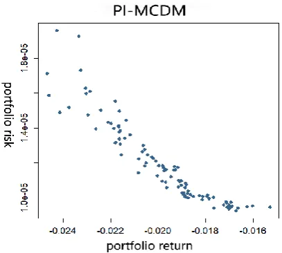
The PI-MCDM progressively interactive decision-making method, through interaction with DMs, obtains their investment preferences and obtains a preference model for investment decisions. Under the guidance of the preference model, the evolutionary algorithm evolves in the direction of DMs' preference. Fig.1 shows the initialized population, which is relatively dispersed in the objective space. After the evolution of gen generations, and before interacting with DM, the objective space solution sets after the NSGAII evolution five generations were obtained. PI-MCDM interacts with DM every five generations. During the interaction process, DM needs to input the conservative and expected values of risk and return, and compares the two investment plans, then PI-MCDM can obtain their preference for the portfolio. For each interaction, PI-MCDM obtains the Pareto frontier and marks the point with the class number 1, which is the DM's most preferred point, as shown by the red dots in Fig.2. The points on the same curve represent the Pareto solution sets obtained for each interaction, and the purple points indicate the points of the class number 1 obtained by the last interaction, which are the DM's most preferred investment plans.

It can be seen from the Fig.2 that compared with the initial population, the population evolves in the direction of higher return and risk of the portfolio during the evolution process, indicating that current DM tends to have higher returns. The portfolio return obtained by PI-MCDM in objective space is (0.015, 0.035), and the portfolio risk range is (1×10-5, 5×10-5), while compared with NSGAII evolution 100 generations (the portfolio return range is (0.03, 0.055), and the portfolio risk range is (2×10-5, 1.4×10-4)), as shown in Fig.3, the DM prefers the portfolio with relatively low risk. Therefore, it can be seen that the DM tends to have low-return and low-risk portfolios. His preferred range of return is approximately (0.025, 0.036) and the range of risk that can be tolerated is (1.5×10-5, 4.5×10-5).

Figure 3. Solutions of NSGAII in objective space after 100 generations action.

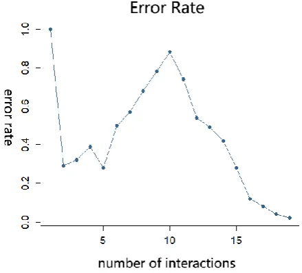
Figure 4. Error rate of the interaction process in PI-MCDM.

Since DMs can be bounded rationality, in the process of interaction, for two sets of candidate solutions, they may not be able to give correct judgement when making decisions, or their investment preference may change as the interaction progresses. Therefore, the error rate of one interaction may be higher than that of the last interaction, indicating the instability of preference. As shown in Fig.4, in the process of interacting with a DM, the overall error rate is declining, but in the 5-10th interaction, the error rate rises.

For portfolio problem, NSGAII will get a set of Pareto solutions through continuous evolution. In the process of evolution, it always evolves towards the direction of maximizing return and minimizing risk. For DMs, the set of solutions obtained may not satisfy their investment preferences, in other word, they cannot choose the most desired investment plan from the solution set. While the progressively interactive decision-making method PI-MCDM, because it considers different DMs have different investment preferences, at the same time, they are bounded rational, through continuous interaction with them, it can determine their investment preferences, then the preference information will be fed back into the evolutionary algorithm, making the evolution direction more in line with the their investment preferences. Compared with NSGAII, PI-MCDM can obtain a set of solutions with a smaller range of portfolio return and portfolio risk, and provide the optimal investment plans.

Conclusion

better reflect DMs' investment preference and find satisfactory solutions that meet their preference, which are satisfactory portfolio plans.

Acknowledgement

This work was supported in part by NSFC under Grant No. 61702139 and NSFS under Grant No. ZR2016FM27.

References

[1] H. Markowitz, Portfolio selection, J. Journal of Finance. 7 (1952) 77-91.

[2] M. Masmoudi, F.B. Abdelaziz, Portfolio selection problem: a review of deterministic and stochastic multiple objective programming models, J. Annals of Operations Research. (2017).

[3] D. Sharma, P. Collet, An archived-based stochastic ranking evolutionary algorithm (asrea) for multi-objective optimization, C. Conference on Genetic & Evolutionary Computation. (2010).

[4] K. Deb, A. Pratap, S. Agarwal, et al. A fast and elitist multi objective genetic algorithm: NSGA-II, J. IEEE Transactions on Evolutionary Computation. 6 (2) (2002) 182-197.

[5] D. Meignan, S. Knust, J.M. Frayret, G. Pesant, N. Gaud, A review and taxonomy of interactive optimization methods in operations research, J. ACM Transactions on Interactive Intelligent Systems (TiiS). 5 (3) (2015) 17.

[6] D. Mukhlisullina, A. Passerini, R. Battiti, Learning to diversify in complex interactive multiobjective optimization, C. Proceedings of the 10th Metaheuristics International Conference. (2013) 230-239.

[7] R. Battiti, A. Passerini, Brain-computer evolutionary multiobjective optimization: a genetic algorithm adapting to the DM, J. IEEE Transactions on Evolutionary Computation. 14 (5) (2010) 671-687.