Volume 2010, Article ID 589618,17pages doi:10.1155/2010/589618
Research Article
Contiguous Extensions of Dixon’s Theorem on
the Sum of a
3F2
Junesang Choi
Department of Mathematics, Dongguk University, Gyeongju 780-714, South Korea
Correspondence should be addressed to Junesang Choi,[email protected]
Received 7 October 2009; Accepted 25 February 2010
Academic Editor: Yeol J. E. Cho
Copyrightq2010 Junesang Choi. This is an open access article distributed under the Creative Commons Attribution License, which permits unrestricted use, distribution, and reproduction in any medium, provided the original work is properly cited.
In 1994, Lavoie et al. have succeeded in artificially constructing a formula consisting of twenty three interesting results, except for five cases, closely related to the classical Dixon’s theorem on the sum of a3F2by making a systematic use of some known relations among contiguous functions.
We aim at presenting summation formulas for those five exceptional cases that can be derived by using the same technique developed by Bailey with the help of Gauss’s summation theorem and generalized Kummer’s theorem.
1. Introduction and Preliminaries
The generalized hypergeometric seriespFqis defined bysee1, page 73
pFq
α1, . . . , αp;
β1, . . . , βq;
z
∞
n0
α1n· · ·αpn
β1n· · ·βqn
zn
n!
pFqα1, . . . , αp; β1, . . . , βq; z,
1.1
whereλnis the Pochhammer symbol definedforλ∈Cbysee2, pages 2 and 6
λn : ⎧ ⎨ ⎩
1, n0,
λλ1· · ·λn−1, n∈N:{1,2,3, . . .}
Γλn Γλ
λ∈C\Z−
0
,
and Z−0 denotes the set of nonpositive integers and Γλ is the familiar Gamma function. Here p and q are positive integers or zero interpreting an empty product as 1, and we assume for simplicity that the variable z, the numerator parameters α1, . . . , αp, and the
denominator parametersβ1, . . . , βq take on complex values, provided that no zeros appear
in the denominator of1.1, that is,
βj/∈Z−0; j1, . . . , q
. 1.3
Thus, if a numerator parameter is a negative integer or zero, thepFqseries terminates in view
of the identitysee2, page 7
−nk
⎧ ⎪ ⎪ ⎨ ⎪ ⎪ ⎩
−1k n!
n−k! , 0≤k≤n; n∈N, 0, k > n.
1.4
In fact,pFqis a natural generalization of the hypergeometric functionor series
2F1 a, b; c; z 2F1
a, b c
z
Fa, b; c; z. 1.5
Gauss proved his famous summation theoremsee1, page 49, Theorem 18
2F1a, b; c; 1 ΓcΓc−a−b
Γc−aΓc−b
Rc−a−b>0; c /∈Z−0.
1.6
Kummer presented the summation theorem for2F1−1 see1, page 68, equation1
2F1
a, b
1a−b −1
Γ1a−bΓ1/2
2aΓ1 1/2a−bΓ1/2 1/2a
Rb<1; 1a−b /∈Z−0.
1.7
Dixon gave the following classical summation formula for3F21 see1, page 92:
3F2
a, b, c
1a−b, 1a−c 1
Γ1a/2Γ1a−bΓ1a−cΓ1a/2−b−c Γ1aΓ1a/2−bΓ1a/2−cΓ1a−b−c, 1.8
Lavoie et al. 3 presented a general, artificially constructed, form of the Dixon’s theorem1.8:
fi,ja, b, c: 3F2
a, b, c
1a−bi, 1a−cij 1
i−3,−2,−1,0,1,2; j0,1,2,3
1.9
by making a systematic use of the relations among contiguous functions given by Rainville
1, page 80, except for the cases
i, j 3,1, 3,2, 3,3, 2,3, and 1,3. 1.10
Very recently, Kim and Rathie4derived twenty five transformation formulas in the form of a single identity for the hypergeometric seriesX8 introduced by Exton by making use of generalized Watson’s theorem5.
Here, in order to present the five exceptional formulas not given by Lavoie et al.3, equation2, page 268, we will first give further extension tables, as inLemma 1.1, of the generalized formulas of the Kummer’s theorem1.7obtained by Lavoie et al.6and then derive the summation formulas of
Ii,ja, b, c ΓaΓbΓc
Γ1a−biΓ1a−cijfi,ja, b, c 1.11
for the cases in1.10, by using the same technique developed by Bailey7with the help of Gauss’s theorem1.6and some identities inLemma 1.1.
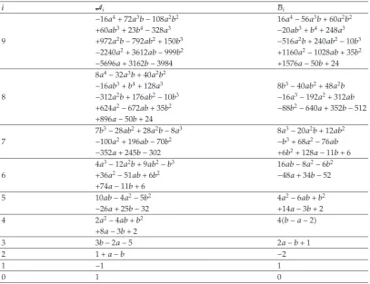
Lemma 1.1. One gives further extension tables of the generalized formulas of the Kummer’s theorem 1.7obtained by Lavoie et al. [6]:
2F1
a, b
1a−bi −1
Γ1/2Γ1−bΓ1a−bi
2aΓ1−bi/2|i|/2
·
Ai
Γa/2−bi/21Γa/2i/21/2−1i/2
Bi
Γa/2−bi/21/2Γa/2i/21/2−i/2
.
1.12
Table 1:Table forAiandBi.
i Ai Bi
−16a472a3b−108a2b2 16a4−56a3b60a2b2
60ab323b4−328a3 −20ab3b4248a3
9 972a2b−792ab2150b3 −516a2b240ab2−10b3
−2240a23612ab−999b2 1160a2−1028ab35b2
−5696a3162b−3984 1576a−50b24
8a4−32a3b40a2b2
−16ab3b4128a3 8b3−40ab248a2b
8 −312a2b176ab2−10b3 −16a3−192a2312ab
624a2−672ab35b2 −88b2−640a352b−512
896a−50b24
7b3−28ab228a2b−8a3 8a3−20a2b12ab2
7 −100a2196ab−70b2 −b368a2−76ab
−352a245b−302 6b2128a−11b6
4a3−12a2b9ab2−b3 16ab−8a2−6b2
6 36a2−51ab6b2 −48a34b−52
74a−11b6
5 10ab−4a2−5b2 4a2−6abb2
−26a25b−32 14a−3b2
4 2a2−4abb2 4b−a−2
8a−3b2
3 3b−2a−5 2a−b1
2 1a−b −2
1 −1 1
0 1 0
Proof. It is not difficult, even though a little complicated, to prove the identities given here by making a main use of the following contiguous relationsee1, equation15, page 71:
c−1 ab1−2czF c−11−zFc−−1
c c−ac−bzFc. 1.13
2. Further Contiguous Extension Formulas of
1.8
In the sake of a little brevity, summation formulas ofIi,ja, b, care given for the cases1.10.
Theorem 2.1. Without restrictions for each formula, one just gives the above-mentioned summation formulas:
I3,1a, b, c α3,1Γb−3Γc−4Γ1/2a1/2Γ1/2a−b−c9/2
Γa−b−c5Γ1/2a−b5/2Γ1/2a−c7/2
β3,1Γb−3Γc−4Γ1/2a1/2Γ1/2a−b−c5
Γa−b−c5Γ1/2a−b2Γ1/2a−c3
γ3,1Γb−3Γc−4Γ1/2a1/2
Γa−b−c5Γ1/2a1 δ3,1
Γb−3Γc−4
Γa−b−c5,
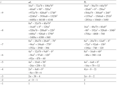
Table 2:Table forAiandBi.
i Ai Bi
16a4−72a3b108a2b2 16a4−56a3b60a2b2
−60ab39b4−320a3 −20ab3b4−256a3
−9 972a2b−828ab2174b3 564a2b−300ab226b3
2240a2−3936ab1323b2 1376a2−1568ab251b2
−6400a4614b6144 −2816a1066b1680
8a4−32a3b40a2b2
−16ab3b4−128a3 16a3−48a2b40ab2
−8 328a2b−208ab222b3 −8b3−192a2328ab−104b2
688a2−928ab179b2 704a−480b−768
−1408a638b840
8a3−28a2b28ab2−7b3 8a3−20a2b12ab2−b3
−7 −96a2196ab−77b2 −72a292ab−15b2
352a−294b−384 184a−74b−120
4a3−12a2b9ab2−b3 8a2−16ab6b2
−6 −36a257ab−12b2 −48a38b64
92a−47b−60
−5 4a2−10ab5b2 4a2−6abb2
−24a25b32 −16a7b12
−4 2a2−4abb2 4a−b−2
−8a5b6
−3 2a−3b−4 2a−b−2
−2 a−b−1 2
−1 1 1
where
α3,1 a−2a−c1
a
2 −b−c 9 2
a
2 −b−c 11
2
1
2b−3c−44a−3c3 a
2 −b−c 9 2
1
2b−2b−3c−3c−4,
β3,1
2
ac−a−1a−1
a
2 −b−c5
,
γ3,1
2
3b−1b−2b−3c−2c−3c−4 a−c2b−2b−3c−3c−4
1
2
c−11−2a 2a2b−3c−4 1
2a−1a−2a−c1,
δ3,1−
22a3
3a1a3b−1b−2b−3c−2c−3c−4
c−4a−2b−2b−3c−3c−4 1
2a−1a−2c−1
1
2b−3c−4{c−12a−1−4a},
I3,2a, b, c α3,2Γb−3Γc−5Γ1/2a1/2Γ1/2a−b−c11/2
Γa−b−c6Γ1/2a−b5/2Γ1/2a−c9/2
β3,2Γb−3Γc−5Γ1/2a1/2Γ1/2a−b−c5
Γa−b−c6Γ1/2a−b2Γ1/2a−c4
γ3,2Γb−3Γc−5Γ1/2a1/2
Γa−b−c6Γ1/2a1 δ3,2
Γb−3Γc−5
Γa−b−c6,
2.3
where
α3,2{c−12a−c2−aa1}a−2
a
2 −b−c 13
2 a
2 −b−c 11
2
1
2{c−18a−3c6−5aa1}b−3c−5 a
2 −b−c 11
2
1
44c−5a−9b−2b−3c−4c−5,
β3,2 a
1
2a2b−2b−3c−4c−5
2
ac−2−2ac−1
2a12
a2
a−1a
2 −b−c5 a
2 −b−c6
1
ac−1c−2 41−c
3a12
a2
b−3c−5a
2 −b−c5
,
γ3,2 a−
11−cc−2
2a aa−2 2b−2c−5{1 b−2c−4}
1−cc−2b−3c−5
2a {a2b−2c−4}
2b−3ac−1c−5
2 aa2 2b−2c−4{a2 b−1c−3}
2a−a1c−1
2
aa 2
2 {a−22b−3c−5}
b−2b−3c−4c−5
a22
3b−1c−3
−a1b−2b−3c−4c−5
2a22a4
×a2a4 2b−1c−3{a4bc−2}
−3a12b−3c−5
2a22a4
a2a4{a2b−2c−4}
2b−1b−2c−3c−4
a42
1−aa12
2a22a4
aa2a4{a−22b−3c−5}
2b−2b−3c−4c−5
×
a2a4 2
3a4b−1c−3
1
3bb−1c−2c−3
,
δ3,2 a−2c−1c−2
2a1 a−1a1 2b−3c−5{a1 b−2c−4}
3b−3c−1c−2c−5
2a1 {a12b−2c−4}
2b−2b−a31−cc−4c−5
1a3 {a32b−1c−3}
4ab−31−cc−5
a1a3 a1a3 2b−2c−4{a3 b−1c−3}
2aaa−21−c
1a3
a1a3
1
2a−1 b−3c−5
b−2b−3c−4c−5
a32
3b−1c−3
5b−2b−3c−4c−5
2a3a5 a3a5 2b−1c−3{a5bc−2}
5ab−3c−5
2a3a5
a5{a1a3 2a2b−2c−4}
2b−1b−2c−3c−4
a52
3bc−2
aaa−2
3a5
a1a3a5
1
2a−1 b−3c−5
a3a5b−2b−3c−4c−5
1
3b−1b−2b−3c−3c−4
× c−5{2a5 bc−2}
I3,3a, b, c α3,3Γb−3Γc−6Γ1/2a1/2Γ1/2a−b−c11/2
Γa−b−c7Γ1/2a−b5/2Γ1/2a−c11/2
β3,3Γb−3Γc−6Γ1/2a1/2Γ1/2a−b−c6
Γa−b−c7Γ1/2a−b2Γ1/2a−c5
γ3,3Γb−3Γc−6Γ1/2a1/2
Γa−b−c7Γ1/2a1 δ3,3
Γb−3Γc−6
Γa−b−c7,
2.4
where
α3,3
a
2 −b−c 11
2 a
2 −b−c 13
2 a
2 −b−c 15
2
·a−21−cc2−3ac2a−5c2aa1a−c3
1
2b−3c−6 a
2 −b−c 11
2 a
2 −b−c 13
2
×aa16a−5c17 1−c3c2−5c24a2−3c
1
4b−2b−3c−5c−6 a
2 −b−c 11
2
· {2c−13c−2 a19a−5c23}
1
4a1b−1b−2b−3c−4c−5c−6,
β3,321−a
a
2 −b−c6 a
2 −b−c7
·
c−13c−2 a−c3a1
2 a2
21−cb−3c−6a
2 −b−c6
3c−2−3a1
a2
a1
2a2b−2b−3c−5c−6c−3a−7−4a1
2b−3c−6,
γ3,3
1
2a1b−2b−3c−5c−6
· {a1a−c4 1−ca−6c6 3}
ab−3c−6
ac−13c−2 a13a1
22a11−c
2a2
1
2aa−1a−2
c−13c−2 a1
2a−c3 a2
δ3,3 b−2b−3c−5c−6
×c−1c2−5c2 a11−c3c−2
1
2c−1
2a26a5− 1 2a2
2a28a9
1
2b−3c−6
1−c2a23c−2−2a1
aa1{2a1c−1−2a1a2}
1
2a−1a−2
c−1c2−5c2aa−3c3−aa2,
I2,3a, b, c α2,3 Γb−
2Γc−5Γ1/2aΓ1/2a−b−c9/2
Γa−b−c6Γ1/2a−b3/2Γ1/2a−c9/2
β2,3 Γb−
2Γc−5Γ1/2aΓ1/2a−b−c5
Γa−b−c6Γ1/2a−b2Γ1/2a−c5
γ2,3 Γb−
2Γc−5Γ1/2a
Γa−b−c6Γ1/2a1/2δ2,3
Γb−2Γc−5
Γa−b−c6,
2.5
where
α2,3
1 2
c2−5c13a21−ca−4c5
4a1
a
2 −b−c 9 2
a
2 −b−c 11
2
3a1−ca−2c3
4a1
aa2
4a3{2a22a3 b−1c−4}
·b−2c−5 a
2 −b−c 9 2
,
β2,3
1 2
a−1c2−5c1−3ac−1a−1c−1−a22a4
·a
2 −b−c5 a
2 −b−c6
1
2
c2−5c13
2ac−14a−3c7− 5
2aa1a2
1
γ2,3 b−2c−5
c2−5c1−3ac−12
2a1 2a1
3
4aa1c−1−
3aa22 2a3
12a
3
a−1
2
c2−5c13a2c−1a−4c5
4a1 −
a2a22 a3
,
δ2,3 b−2c−5
−a1c2−5ca3
22a1c−1
2
31−ca2−21
2a2
2a2a−7
1
21−a
c2−5c1
a
2
3a−1c−1231−ca2−2a4 a2a2−2a−6,
I1,3a, b, c α1,3Γb−
1Γc−4Γ1/2a1/2Γ1/2a−b−c7/2
Γa−b−c5Γ1/2a−b3/2Γ1/2a−c9/2
β1,3Γb−
1Γc−4Γ1/2a1/2Γ1/2a−b−c4
Γa−b−c5Γ1/2a−b1Γ1/2a−c4
γ1,3Γb−
1Γc−4Γ1/2a1/2
Γa−b−c5Γ1/2a δ1,3
Γb−1Γc−4
Γa−b−c5,
2.6
where
α1,3
1 2
a
2 −b−c 7 2
a
2 −b−c 9 2
·aa1a22−c2−5c13a1−c2−ca
1
4b−1c−4 a
2 −b−c 7 2
·6c−129a11−c 4a1a2
1
4a1bb−1c−3c−4,
β1,3
a
2 −b−c4
·
c2−5c1
a −3c−12
a12
a2 3c−a−5
3aa12c−1
2
a1
γ1,3−c
2−5c1
a 3c−12−
a3c−1a12
a2 ,
δ1,3
1 2
c2−5c13
2ac−1a−c2− 1
2aa1a2
2.
2.7
3. Proof of
Theorem 2.1
We will prove onlyI3,2a, b, c. The other formulas in Theorem 2.1can be shown as in the
proof ofI3,2a, b, c. We begin by writing
I3,2a, b, c
∞
n0
ΓanΓbnΓcn
n!Γ4a−bnΓ6a−cn
∞
n0
ΓanΓbnΓcn
n!Γ4a−bnΓ6a−cn·
Γa2n4Γa−b−c6
Γa2n4Γa−b−c6,
3.1
by which the bold face factors are multiplied. Rearranging the factors in the last sum to use the Gauss’s summation theorem1.6, we get
I3,2a, b, c
∞
n0
ΓanΓbnΓcn
n!Γa2n4Γa−b−c6·
Γa2n4Γa−b−c6
Γ4a−bnΓ6a−cn
∞
n0
ΓanΓbnΓcn
n!Γa2n4Γa−b−c6·2F1
bn, c−2n
a2n4 1
.
3.2
Rewriting the last 2F1and using a manipulation of double series, we obtain
I3,2a, b, c
∞
n0
∞
m0
c−1nc−2nΓanΓbnmΓc−2nm
n!m!Γa−b−c6Γa42nm
∞
m0
m
n0
c−1nc−2nΓanΓbmΓc−2m
n!m−n!Γa−b−c6Γa4nm
·Γam!Γa4m
Γam!Γa4m.
∞
m0
ΓbmΓc−2mΓa
m!Γa−b−c6Γa4m
·m n0
m!c−1nc−2nΓanΓa4m
m−n!n!ΓaΓa4mn .
Separating the last summation, we find that
I3,2a, b, c
∞
m0
ΓbmΓc−2mΓa
m!Γa−b−c6Γa4m
· {c−1c−2Pa, m 2c−1Qa, m Ra, m},
3.4
where
Pa, m m
n0 m!
n!m−n!
ΓanΓa4m
ΓaΓa4mn,
Qa, m m
n0
m!n
n!m−n!
ΓanΓa4m
ΓaΓa4mn,
Ra, m m
n0
m!nn−1
n!m−n!
ΓanΓa4m
ΓaΓa4mn.
3.5
Using1.2and1.4to expressPa, m,Qa, m, andRa, min the forms of 2F1−1,
3.4is rewritten as follows:
I3,2a, b, c Aa, b,c Ba, b, c Ca, b, c, 3.6
where
Aa, b, c c−1c−2Γa
Γa−b−c6 ∞
m0
ΓbmΓc−2m
m!Γa4m 2F1
a, −m a4m
−1
,
Ba, b, c 2c−1Γa1
Γa−b−c6 ∞
m0
mΓbmΓc−2m
m!Γa5m
·2F1
a1, 1−m
a5m −1
,
Ca, b, c Γa2
Γa−b−c6 ∞
m0
mm−1ΓbmΓc−2m
m!Γa6m
·2F1
a2, 2−m
a6m −1
.
3.7
Applying some appropriate formulas inLemma 1.1to 2F1−1in3.6, we obtain
Aa, b, c 4
j1
where
A1a, b, c a−
21−cc−2Γa/21/2
Γa−b−c6
×
⎡ ⎢
⎣ΓΓba/−32Γ−1c/−25·2F1
⎡ ⎢ ⎣
b−3, c−5
a
2 − 1 2
1
⎤ ⎥
⎦−Γb−3Γc−5
Γa/2−1/2
− Γb−2Γc−4
Γa/21/2 −
Γb−1Γc−3 2Γa/23/2
⎤ ⎥ ⎦,
A2a, b, c 31−cc−2Γa/21/2
2Γa−b−c6
×
Γb−2Γc−4
Γa/21/2 ·2F1
b−2, c−4
a/21/2 1
− Γb−2Γc−4
Γa/21/2 −
Γb−1Γc−3
Γa/23/2
,
A3a, b, c
2a−1c−1c−2Γa/21/2
aΓa−b−c6
×
⎡
⎣Γb−3Γc−5
Γa/2−1 ·2F1 ⎡
⎣ b−a3, c−5 2 −1
1
⎤
⎦−Γb−3Γc−5
Γa/2−1
− Γb−2Γc−4
Γa/2 −
Γb−1Γc−3 2Γa/21
⎤ ⎥ ⎦,
A4a, b, c c−
1c−2Γa/21/2
aΓa−b−c6
×
⎡ ⎢
⎣Γb−2Γc−4
Γa
2
·2F1
⎡
⎣ b−2, ca −4 2
1
⎤ ⎦
− Γb−2Γc−4
Γa/2 −
Γb−1Γc−3
Γa/21 ⎤ ⎦,
3.9
Ba, b, c 5
j1
where
B1a, b, c c−
1Γa/21/2
Γa−b−c6
×
⎡ ⎢
⎣ΓΓba/−12Γ3c/−23·2F1
⎡ ⎢ ⎣
b−1, c−3
a
2
3 2
1
⎤ ⎥ ⎦
− Γb−1Γc−3
Γa/23/2 −
ΓbΓc−2
Γa/25/2 ⎤ ⎥ ⎦,
B2a, b, c
4ac−1Γa/21/2
Γa−b−c6
×
⎡ ⎢
⎣ΓΓba/−22Γ1c/−24·2F1
⎡ ⎢ ⎣
b−2, c−4
a
2
1 2
1
⎤ ⎥
⎦−Γb−2Γc−4
Γa/21/2
− Γb−1Γc−3
Γa/23/2 −
ΓbΓc−2 2Γa/25/2
⎤ ⎥ ⎦,
B3a, b, c
2aa−2c−1Γa/21/2
Γa−b−c6
×
⎡ ⎢
⎣ΓΓba/−32Γ−1c/−25·2F1
⎡ ⎢ ⎣
b−3, c−5
a
2 − 1 2
1
⎤ ⎥
⎦−Γb−3Γc−5
Γa/2−1/2
− Γb−2Γc−4
Γa/21/2 −
Γb−1Γc−3 2Γa/23/2 −
ΓbΓc−2 6Γa/25/2
,
B4a, b, c
41−cΓa/21/2
Γa−b−c6
×
⎡
⎣Γb−2Γc−4
Γa/2 ·2F1 ⎡
⎣ b−2, ca −4 2
1
⎤
⎦−Γb−2Γc−4
Γa/2
− Γb−1Γc−3
Γa/21 −
ΓbΓc−2 2Γa/22
B5a, b, c 4a−11−cΓa/21/2
Γa−b−c6
×
⎡
⎣Γb−3Γc−5
Γa/2−1 ·2F1 ⎡
⎣ b−a3, c−5 2 −1
1
⎤
⎦−Γb−3Γc−5
Γa/2−1
− Γb−2Γc−4
Γa/2 −
Γb−1Γc−3 2Γa/21 −
ΓbΓc−2 6Γa/22
⎤ ⎥ ⎥ ⎦.
3.11
Ca, b, c 6
j1
Cja, b, c, 3.12
where
C1a, b, c −
5a1 4
Γa/21/2
Γa−b−c6
×
⎡ ⎢
⎣ΓΓba/−12Γ3c/−23·2F1
⎡ ⎢ ⎣
b−1, c−3
a
2
3 2
1
⎤ ⎥
⎦−Γb−1Γc−3
Γa/23/2
− ΓbΓc−2
Γa/25/2−
Γb1Γc−1 2Γa/27/2
⎤ ⎥ ⎦,
C2a, b, c −5aa1
2
Γa/21/2
Γa−b−c6
×
⎡ ⎢ ⎢
⎣Γb−2Γc−4
Γ
a
2
1 2
·2F1
⎡ ⎢ ⎣
b−2, c−4
a
2
1 2
1
⎤ ⎥
⎦−Γb−2Γc−4
Γa/21/2
− Γb−1Γc−3
Γa/23/2 −
ΓbΓc−2 2Γa/25/2−
Γb1Γc−1 6Γa/27/2
C3a, b, c −aa−2a1Γa/21/2
Γa−b−c6
×
⎡ ⎢
⎣ΓΓba/−32Γ−1c/−25·2F1
⎡ ⎢ ⎣
b−3, c−5
a 2 − 1 2 1 ⎤ ⎥
⎦− Γb−3Γc−5
Γa/2−1/2
− Γb−2Γc−4
Γa/21/2 −
Γb−1Γc−3 2Γa/23/2 −
ΓbΓc−2 6Γa/25/2−
Γb1Γc−1 24Γa/27/2
⎤ ⎥ ⎦,
C4a, b, c a1
2a2
Γa/21/2
Γa−b−c6
×
⎡
⎣Γb−1Γc−3
Γa/21 ·2F1 ⎡
⎣ b−a1, c−3 2 1
1
⎤
⎦− Γb−1Γc−3
Γa/21
− ΓbΓc−2
Γa/22 −
Γb1Γc−1 2Γa/23
⎤ ⎥ ⎦,
C5a, b, c
3a12
a2
Γa/21/2
Γa−b−c6
×
⎡
⎣Γb−2Γc−4
Γa/2 ·2F1 ⎡
⎣ b−2, ca −4 2
1
⎤
⎦− Γb−2Γc−4
Γa/2
− Γb−1Γc−3
Γa/21 −
ΓbΓc−2 2Γa/22 −
Γb1Γc−1 6Γa/23
⎤ ⎥ ⎦,
C6a, b, c 2a−1a1 2 a2
Γa/21/2
Γa−b−c6
×
⎡
⎣Γb−3Γc−5
Γa/2−1 ·2F1 ⎡
⎣ b−a3, c−5 2 −1
1
⎤
⎦− Γb−3Γc−5
Γa/2−1
− Γb−2Γc−4
Γa/2 −
Γb−1Γc−3 2Γa/21 −
ΓbΓc−2 6Γa/22 −
Γb1Γc−1 24Γa/23
⎤ ⎥ ⎦.
3.13
We conclude this paper by noting that by extending Tables1and2and using the same technique given here, all other known formulas in3 see1.9can be proved and further extension summation formulas forfi,ja, b, cin1.9
i, j∈Z\ {−3,−2,−1,0,1,2} ×N0\ {0,1,2,3}
3.14
can be presented, whereN0:N∪ {0}andZdenotes the set of integers.
References
1 E. D. Rainville,Special Functions, The Macmillan, New York, NY, USA, 1960.
2 H. M. Srivastava and J. Choi,Series Associated with the Zeta and Related Functions, Kluwer Academic Publishers, Dordrecht, The Netherlands, 2001.
3 J. L. Lavoie, F. Grondin, A. K. Rathie, and K. Arora, “Generalizations of Dixon’s theorem on the sum of a3F2,”Mathematics of Computation, vol. 62, no. 205, pp. 267–276, 1994.
4 Y. S. Kim and A. K. Rathie, “On an extension formulas for the triple hypergeometric seriesX8due to
Exton,”Bulletin of the Korean Mathematical Society, vol. 44, no. 4, pp. 743–751, 2007.
5 J. L. Lavoie, F. Grondin, and A. K. Rathie, “Generalizations of Watson’s theorem on the sum of a3F2,” Indian Journal of Mathematics, vol. 34, no. 2, pp. 23–32, 1992.
6 J. L. Lavoie, F. Grondin, and A. K. Rathie, “Generalizations of Whipple’s theorem on the sum of a3F2,” Journal of Computational and Applied Mathematics, vol. 72, no. 2, pp. 293–300, 1996.