Three stage Iterative Trajectory Association Extraction Technique Based on Improved Track Initiation Model

2019 International Conference on Computer Science, Communications and Big Data (CSCBD 2019) ISBN: 978-1-60595-626-8

Three-stage Iterative Trajectory Association Extraction Technique

Based on Improved Track Initiation Model

Yi

-

fan WU

, Jun JIANG, Xiao

-

min RAN, Jing ZHANG,

Guang

-

ya ZHANG and Ming

-

xuan LI

National Digital Switching System Engineering and Technology Research Center, Zhengzhou 450002, P.R. China

*Corresponding author

Keywords: Track initiation model, Track initiation model, Trajectory association extraction

technique.

Abstract. This article puts forward the improvement of dynamic extrapolation rule combining track initiation process, and then to improve the process of track initiation model. Meanwhile, it adds the measurement interval judgment and quality management, as well as puts forward three stages associated iteration trajectory extraction algorithm of the overall process.

Introduction

It can obtain the rule information of the target motion that analyze the positioning data, and then predict and track the target motion. However, in practical multi-target passive location applications, multiple targets often have the same signal characteristics, and it is difficult to distinguish the target by the signal characteristics. Therefore, it is of great significance to accurately distinguish multiple targets by merely locating the time and location information of the results, and then extract the trajectory of the target. This is not only the basis and prerequisite for further analysis of the positioning data, but also the ability to predict the movement of the target, so as to provide the basis for subsequent positioning.

In this article, aiming at the problem that the positioning period is not fixed in the passive location scenario, the algorithm of the track initiation algorithm is improved, and the accuracy of the trajectory extraction of the trajectory crosses, the historical trajectory extraction and the real-time tracking need to coexist is further optimized. A practical three-stage iterative trajectory extraction algorithm for multi-target positioning data is proposed. Based on the traditional track initiation logic method0, the algorithm first adds measurement intervals before each batch of data matches the existing trajectory to reduce the impact of measurement cycles; secondly, when the temporary trajectory is established, consider the included angles in the trajectory direction, and pre-screening is performed to reduce the splitting of false trajectories when the cross trajectory is extracted. Finally, a trajectory extraction framework is proposed, and a dynamic extrapolation rule is established using the Singer model, which not only satisfies the requirements for historical data analysis, but also is suitable for real-time tracking application. Simulation test results show that the algorithm can achieve the trajectory extraction function of passive location data. The accuracy of the trajectory extraction is higher than in the traditional method when the positioning point is lost. When the proportion of maneuvering target is high in the target of the extracted trajectory, the dynamic extrapolation error far less than a linear extrapolation method.

Improved Dynamic Extrapolation Rule

Observation Model and Target Movement Model

Observation Model. There are numerous passive location methods and observation models are different. In this section, the most commonly used multi-station direction finding method for target monitoring is adopted. The observation station and the target are located on the ground plane. The signal propagates along the line of sight without considering the effect of the curvature of the earth.Let the target position be U[x, y]T , the observation station position is [x , y_{i i}]T ,and the orientation degree measured is _i, The distance from the observation station i to the reference point is D_0i.The angle is _0i:

0 0

0 0

0 0

sin i , cos i( 1, 2,..., )

i i

i i

y y x x

i N

D D

 

     (1)

Where

2 2 1/2 0i [(x0 x )i (y0 y ) ]i

D    

(2) The least squares estimate of the target position is:

T 1 -1 T -1

0 r

ˆ = +(  )

U U G G G N Φ (3) Where

01 01 01 01

0 0 0 0

(sin ) / (cos ) /

... ...

(sin N) / N (cos N) / N

D D D D                   G (4)

N_{is the deviation covariance matrix for each observation station's orientation measurement error,}

and the orientation error is set as an independent random variable with a variance of ,

2 1 2 0 0 _N                N (1)

Covariance matrix of ˆU

1 12 21 2            R The element values are:

2 2

1= [(E x - xˆ ) ]= 2  

  ₍₂₎

2 2

2= [(E y - yˆ ) ]= 2  

  ₍₃₎

2 2

12= 21= [(E x - x y - yˆ )(ˆ )]= 2   

2 0 2 2 0 cos N i

i Di i

 _  



i Di i

 _  



i Di i





 





(7)

Let the system state vector

x y x y x y           

X , Then the observation equation at time k is:

( )k  ( )k  ( )k

Z HX R ₍₈₎

The measurement matrix

[1, 0, 0] 

H ₍₉₎ Sports Model. Because the passive location data contains maneuvering targets, such as aircraft, where the acceleration can quickly change, and non-maneuvering targets, such as ships, etc., it is necessary to adopt a target motion model that can adapt to multiple motion modes. The Singer model was proposed by R. A. Singer in 1970. The acceleration a(t) = [x, y] of the target was considered to be a zero-mean random process0, namely:

2 2

( ) [ (t) T(t )] x y

a mx my

R  Ea a   e   e 

(10) Let x and y be independent and identically distributed, which can be simplified as

2 ( ) [ (t) T(t )]

a m

R  E a a   e 

(11) Where is the acceleration variance of the target, α is the reciprocal of the maneuvering time constant, the physical meaning is the maneuver frequency, and usually the targets of different maneuvering capabilities will have different empirical values0.

Then, the maneuvering model control term is modeled as correlated noise, and the temporal correlation function Ra(τ) of the above formula is whitened, and the time-dependent model with white noise input is expressed as:

( )t   ( )t v t( )

a a ₍₁₂₎

In the above equation, (t) is a mean of 0 and a variance of Gaussian white noise with 2α . The state equation of the Singer model is expressed as:

( )t  ( )t  ( )t

X AX V ₍₁₃₎

System matrix

0 1 0 0 0 1 0 0 A           

  ₍₁₄₎ Process noise

T

[0, 0, ]v



Set the bit interval time to T and the dynamic equation is:

(k 1) ( ) ( )k k  ( )k

X F X V ₍₁₆₎

2

1 ( 1 ) /

0 1 (1 ) /

0 0

T

AT T

T

T T e

e e e                 _  _     F (17) The covariance of the process noise V is

11 12 13 2

21 22 23 31 32 33 2 m

q q q

q q q

q q q

      _{ }     Q (18) The value of qij is in standard form. See literature0.

Dynamic Extrapolation Rules

When the track initiation model is used for trajectory extraction, the length of the intermediate trajectory varies from two to more points, the number of correlations performed is also different, and the reliable trajectory is more than three points. For different phases, the need for accuracy varies0. The Singer model can describe the targets of different maneuvering features, but it has a large amount of computation. When the amount of data is small, the cost of the calculated cost is low0. Starting from the above two points, this paper proposes that different extrapolation rules should be adopted for different trajectory extraction stages. The direction finding and position is mostly aimed at the coast or sea targets. The maneuvering characteristics of the aircraft and the ship are significantly different, and their movement speeds are very different. Therefore, it is the premise for accurate tracking that the speed can better distinguish the target maneuverability and set different Singer model maneuvering parameters.

For the middle trajectory, extrapolate the line at a constant speed and set all the position points obtained at time Zi. The extrapolation rule is:

1 ˆ _{( ) /}

i  i i ti

V Z Z

(19)

1/ 1

ˆ ˆ

i i  i i ti

Z Z V

(20) For a reliable trajectory, its velocity i is first calculated. If it is less than 80 Km/h, it is regarded as a non-maneuvering target such as a vessel or a vehicle. The Kalman filter is performed using a linear motion model; if it is greater than 80 km/h, it is considered as a high-speed maneuvering target for aircrafts. Using the Singer model to perform the Kalman filter iterative extrapolation, the algorithm is as follows.

Calculate the prediction state and covariance matrix:

1| |

ˆ ˆ

i i  i i

X FX

(21) T

1|i i|i i 1

i   

P FP F Q

(22) Calculate observation forecasts, information variance matrix, and Kalman filter gains:

1| 1|

ˆ ˆ

ii  i i

Z HX

(23)

1 1|

T

i  ii 

S HP H R

1 1 1| 1

T

i+ i i i



 



K P H S

(25) After the arrival of the new i + 1 positioning results, calculate the posterior state and variance matrix:

1| 1 1| 1 1 1|

ˆ ˆ ₍ ˆ ₎

i i  ii  i i  i i

X X K Z Z

(26)

1| 1 ( 1 ) 1|

i i   i i i

P I K H P

(27) Iteratively loops in turn, where F, Q are defined in 3.1.1 (21) (22), H, and R is defined in 3.1.1 (15) (13)

Dynamic extrapolation decision flow chart is as figure 1:

Figure 1. Dynamic extrapolation process

Improved Track Initiation Model

Measurement Interval Judgment

The traditional track initiation model is divided into 3 steps: 1. establishing the track head; 2. starting the middle track; 3. confirming the middle track and establishing a reliable track. The quality of these three tracks increases in turn depending on the number of points on the association. Therefore, when processing the positioning points at each time, the association is performed in descending order of quality. Firstly, the obtained positioning points are processed in chronological order. The points at time i are firstly related to the reliable tracks that have been formed, and the associated successful points are used to update the reliable track, and the remaining track marks and the formed temporary track. Related unsuccessful links are used to update the temporary track header. In normal radar, the track head is difficult to select because the new target in the radar power zone is mixed with the false detection caused by noise, interference, and clutter. However, this problem does not exist in the direction finding positioning and can be directly selected that associate the point on the temporary and reliable track as the head of the track.

For the problem that the measurement period is not fixed, this paper further optimizes the above processing framework and designs the following judgment rules: Before the data at each moment in time is related to the trajectory, the time intervals t_i t i( ) t i( 1) between each positioning moment and the previous moment is first calculated, the statistical average of t avg(t_i); then in the course of the trajectory, it is first judged whether t_i exceeds the t or not; Then calculate ( )t i n(r)for each trajectory, if it is greater thant and terminate the trajectory. Where  is a coefficient, determined according to rules of thumb.The reliable track  =3, middle track  =2, track head  =1.

Trajectory Quality Management

trajectory establishes a stable trajectory, the ratio of the modified logic method is used as the quality index. Because the quality of the evaluation trajectory is different in different stages, the quality index of each stage is valid only in the corresponding stage. The stability of the trajectory after the establishment of a reliable trajectory must also be managed by its quality to determine whether the trajectory termination condition has been reached. Otherwise, the poor quality trajectory will interfere with subsequent trajectory extraction and increase the computational burden. Therefore, it is necessary to define the quality index of the reliable trajectory.

Associated Quality Management of Intermediate Trajectories. The correlation of the middle trajectory needs to calculate the distance between the observation point Z_i1at the moment ofi1and the prediction point. The closest observation point is associated with the trajectory, and then it is judged whether the point falls within the relevant wave gate, and the elliptical wave gate is used:

1

1 ˆ 1/ 1/ 1 ˆ 1/ (Z_i Z_{i i})TP_i_{ i}(Z_i Z_{i i})

(28) Where

-1 1

i+ / i

P

is the predictive covariance matrix, the wave gate meets the

2

 _{distribution, and} _{is the}

wave gate threshold. For the measurementzn(i1) _{that falls into the wave gate, the connection} between the measurement and the second point of angle θ of the middle trajectory

(r,2) ( 1) ( )

n i  i

z z

and the original Trajectory line z(r,1)(i1)z(r,2)( )i _{, according to the target} maneuverability, set the turning angle threshold , when  ,think zn(i1) _{is associated with the} trajectory r, because the angle of the small turning speed, requires a strong turning maneuverability, and the target turning maneuverability is limited, adding this kind of judgment can reduce the number of erroneous connections when the trajectory crosses.

When multiple split trajectories l are connected with matching trajectory points, the pruning of the split trajectory is needed. Based on the magnitude of the cumulative error and the included angle, a combination l( ,2) ( ,3)l  l (i 1) {z( ,2)l ( ),i z( ,3)l (i1)} _{of each corresponding point in the trajectory}

and the wave gate is defined. Calculation

1

( ,2) ( ,2)

1

ˆ ˆ

( ) a [ ( 1) ( 1)]T ( 1) [ ( 1) ( 1)]

l l l l

l

C l _ i i i _ i i b





  z  x  R  z  x   

(29) Where a,b are scalar constants and are used to adjust the distance and the weight of the included angle.，xˆ (l i1)_{is the predicted value of the target position at time i +1. Finally take the branch with} the smallest C value as the definite trajectory

*

arg min ( )

l  C l _.

Considering the problem that i +1 may lose the target location point at time, this paper uses a one-step delay algorithm to continue to extrapolate the trajectory r and judge it again according to the above association threshold and included angle threshold. That is, Zi1Zˆi1/i _{brought into the next}

cycle and the correlation is made at the time of i +2. If the correlation is not or t i( 2)t i( ) 2 t , the trajectory is terminated.

Reliable Trajectory Weighted Scoring Quality Management. The quality of the reliable trajectory mainly considers the number of leaked points and the time interval, and adopts an improved weighted scoring method.

The stability trajectory quality Q i_r( )Q i_r(  1) q i_r( ),q i_r( )is scored at time i. The scoring rules are:

(3) If there is no associated positioning point, if t i

   

   

t i t i  t , deduct 2 points; in addition, if i-1 is deducted at any time, i will be deducted 2 times.

By this way of scoring, the quality of the reliable trajectory is managed, the trajectory with poor quality is terminated in time, and part of the traces are also allowed to be lost in the reliable trajectory. It has certain adaptability, and the effect of missing points is higher when the positioning frequency is higher. Small, deducted scores are also less, when the continuous loss of positioning points, the trajectory quality decreased faster.

Trajectory Extraction Process Framework

(1) Track head establishment

As described in introduction, the DF positioning data is different from the radar data, the same target at each time get a positioning result, so free points can be established as track heads. The free points mainly include the following three situations: all the anchor points at the initial moment, not associated with the anchor points in any one track, and When  ti  t _{, the all anchor points of i are}

( )i

Z _{, The established track head is written as} trr {z(r,1)( )}, ri m i( ) (2) Consider the speed constraint to establish the middle trajectory A certain track head (r,1)( )=[ (r,1)( ), (r,1)( )]

x y

j z j z j

  

z

established at time j is taken as the center. According to the target's motion capability, the maximum and minimum distance that can be moved is the circle within the time period of tij= ( )t i t j( )_{, and a confidence region is established. Define the}

distance

(r,1) max (r,1) min

(r,s) max[0, ( ) ( ) ] max[0, ( ) ( ) ]

x x x x x x x

ij s ij s ij

d  z i z_ j v t  z i z_ j v t

(30)

(r,1) max (r,1) min

(r,s) max[0, ( ) ( ) ] max[0, ( ) ( ) ]

y y y y y y y

ij s ij s ij

d  z i z_ j v t  z i z_ j v t

(31) The distance vector is:

(r,s) [ x(r,s), y(r,s)]

ij  dij dij

d

(32) Where ( )t i t j( ) t . Let the measurement error be an independent zero-mean-normal distribution with a covariance matrixRi(r)_{, the squared regularization distance is:}

1

(r,s) T(r,s)[ ( ) ( )] (r,s)

ij ij i j ij

D d R s R r  d

(33) (r,s)

ij

D

obeys a χ2 distribution with 2 degrees of freedom. When z(r,1)( )j _and zs( )i _are

interconnected, Dij(r,s)_{, If multiple points are satisfied at the same time, the trajectory is split}

into multiple segments. Trajectory splitting will lead to a significant increase in computational and storage space usage, but it is also possible to find more possible connections. In practice, the number of direction-finding stations is limited, and the number of target-targets is also limited, so under the existing conditions, It is feasible that all the points falling within the associated threshold start with an intermediate trajectory.

(3) Association of intermediate trajectories

falls within the relevant wave gate; A plurality of split trajectories l are connected with matching trajectory points, and the pruning of split trajectories is required, based on the magnitude of accumulated errors. In this paper, two aspects of intermediate track correlation are improved. First, when predicting the target position at i+1, namely, extrapolating the calculation, the linear extrapolation of traditional linear extrapolation or acceleration expansion is transformed into a dynamic extrapolation algorithm. In the middle trajectory step, the Kalman filter algorithm of the linear motion model is used. Second, in the calculation of the cumulative error, the value of the included angle after the weight adjustment is added to the traditional cumulative error calculation method, and the trajectory extraction accuracy rate when the trajectory crosses is improved.

(4) Establishment of stable track

The 3/4 logic method is often used for fast trajectory initiation. This article uses this method to determine the stability trajectory establishment. In order to make the algorithm have good scalability under real-time tracking conditions. Moreover, the time length of the traditional logic method is fixed. Based on this, the paper improves it, fixes the number of moments and limits the maximum length of the time window, making it more suitable for the scene with a fixed positioning period. For the trace

(r,1) (r, ) (r, ( ))

r { z_ ( ),i z_{ k} ( )j z_{ m r} [ ( )]}n r

, if t n r[ ( )]t i( ), the ratio of the number of positioning points on the association to the number of times the positioning data is obtained during the duration of

the trajectory, if

3 ( ) / [ ( ) 1]

4

m r n r i + 

establishes a reliable trajectory; if any of the above two is not satisfied, the time window is shifted back one moment until a stable track is established or the middle track ends.

Three-stage Iterative Trajectory Extraction Algorithm

This chapter presents the overall flow of the algorithm. Because the passive location monitoring is military-sensitive, there is a lack of currently available references for the extraction of passive location data trajectories. This paper will introduce the track initiation algorithm to the track extraction domain. The track starting model, on the basis of which, removes the definition of the temporary track, adds measurement interval judgment to the characteristics of the passive location cycle, and connects the entire track from the start to the end of the series in series, and proposes an improved track quality. Management sets different extrapolation rules according to the different maneuvering characteristics of the target, forming a three-phase iterative trajectory extraction algorithm.

From the perspective of each positioning moment, the higher the quality of the trajectory. The higher the degree of confidence, in order to avoid low-quality trajectories occupying high-quality trajectory requires the associated positioning point, so the positioning point at each moment is matched with the higher-level trajectory; from the logic of each trajectory, it is gradually related from the low gradient trajectories to. As the associated point traces increase, the extrapolation error decreases, the quality gradually increases, a reliable trajectory is formed, the reliable trajectory continues to be associated (tracking) in the follow-up, and when the positioning point is lost or the tracking of the target is stopped, the quality gradually decline, the final trajectory terminates.

The specific steps of the algorithm are as follows: (0) Calculate the average time interval

Calculate the time interval between each positioning moment and the previous moment ti t i( ) t i( 1) _{, statistical mean}  t avg(t)

(1) Judgment interval

If   ti  t _{, terminate all tracks and go to (7). Calculate ( )}t i n r( ) _{for each trajectory, if it is} more than t , stop the trajectory. Where αis the coefficient, determined according to the rule of thumb, the reliable trajectory =3 , medium Inter-track =2 , track head =1 .

Use the dynamic extrapolation rule to predict the next position of the reliable trajectory, and calculate the observation point and predetermination at time i1 . The distance between measurement points is calculated according to Equation (37), and the correlation is selected by selecting the closest point in the relevant wave gate.

(3) The remaining positioning points are extrapolated using the linear model Kalman filter and are calculated using (23) (24) count, use the methods in 3.2.1 to perform correlation quality calculations and correlate and prune.

(4) Residual positioning point Use the method of step (2) in section 3.3 to establish the intermediate trajectory.

(5) Establish the stable trajectory of the middle trajectory using the method of step (3) (4). (6) The trajectory quality management is performed using the method of Section 3.2.2. (7) The remaining positioning point establishes the trajectory header.

(8) If the positioning point exists at the next moment, turn (1), if it does not exist, then output the trace extraction result, and the algorithm ends.

Simulation Results and Performance Analysis

Simulation Environment Settings

The trajectory extraction simulation scenario is short-wave direction finding and positioning. Four targets perform uniform acceleration motion and one performs uniform-speed linear motion. At each time point, the target stops communications with a certain probability, making the positioning point of this target lost at this moment. The positioning measurement error R satisfies a normal distribution with a mean of 0 and a variance of 25; the target motion acceleration disturbance results in a normal distribution of system error Q satisfying a mean value of 0 and a variance of 10. According to a

2

 _{distribution with a degree of freedom of 2, the probability of 99% is obtained by looking at the}

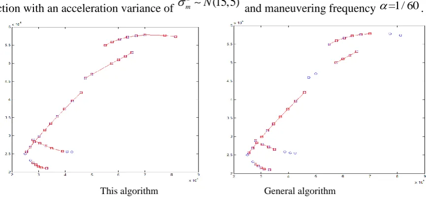
threshold of the gate =9.21 . In the real-time trajectory tracking, 10 simulation targets are generated. The positioning measurement error R satisfies a normal distribution with a mean value of 0 and a variance of 25; the target motion system error Q satisfies a normal distribution with a mean value of 0 and a variance of 10. In order to increase the number of maneuvering targets, the acceleration of the maneuvering target is a zero-mean random process consistent with an exponential autocorrelation function with an acceleration variance of

2

(15,5)

m N



and maneuvering frequency =1/ 60.

This algorithm General algorithm

Analysis of Simulation Results

In Figure 2, the horizontal and vertical coordinates represent the coordinates of the target position.We can see from the above simulation results that, in the scene, where the positioning frequency is not fixed, the correction logic method used in this paper is determined during the trajectory extraction process. When there are missing points in the middle of the locus, the connection of the trajectory can be completed better; when the trajectory crosses, the method of this article can also correctly extract the trajectory.

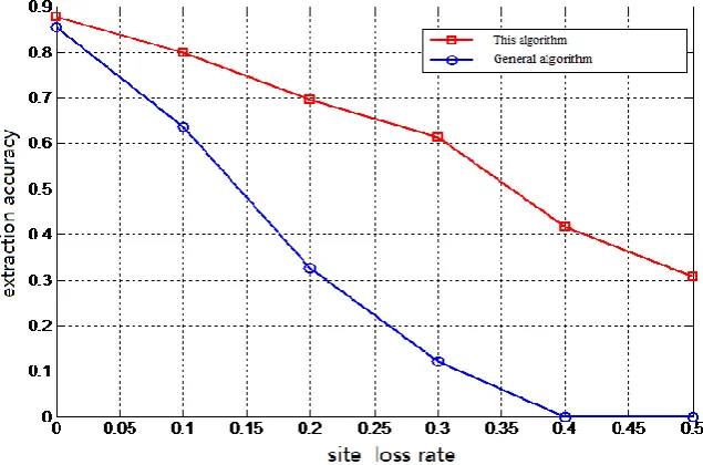
Figure 3. Comparison of trajectory extraction accuracy.

Figure 4. Comparison of root-mean-square error between dynamic extrapolation and linear extrapolation.

Defining the accuracy of trajectory extraction as

100%

c

t

  

, where c _{is the correct number of} connections andt _{is the total connection. The number can be calculated by subtracting the number of} tracks from the total track points. Based on this simulation, we can see from figure 3 that the modified logic method in this paper is more suitable for the passive DF location scenario than the traditional method. When the loss rate of the location point increases, the trajectory is extracted. The correct rate is much higher than the traditional method.

compare to 1 The situation is increased by 30%; when the number of maneuvering targets is 1-3, the linear extrapolation and dynamic extrapolation errors are approximately the same. When the maneuvering target continues to increase, the linear extrapolation error rapidly increases, and when the 10 targets are all maneuvering target, the linear extrapolation error is more than three times the dynamic extrapolation. From the comparison, it can be seen that the dynamic extrapolation rule proposed in this paper has relatively stable extrapolation error when the target maneuverability is uncertain, which is more suitable for the passive location of multi-target mixed scenes.

Conclusion

This paper presents a trajectory extraction algorithm for direction finding data. The algorithm can extract the trajectory in the DF data with unfixed positioning period and more cross trajectory, and maintain better tracking performance during continuous tracking. The algorithm adds measurement interval judgment and combines it with one-step delay algorithm, selects the trajectory points with reasonable positioning interval to connect; when the temporary trajectory and the stable trajectory are formed, the steering angle of the trajectory is constrained, and the wrong connection of the cross trajectory is reduced; and the trajectory starting model is improved. The processing framework of the trajectory extraction problem is proposed for the first time. The dynamic extrapolation rules are introduced to realize the flexible switching of the trajectory extraction and tracking process. The simulation results show that the proposed algorithm can effectively extract the trajectory. Compared with the traditional logic method, the trajectory is extracted directly. When the trajectory is crossed and the positioning point is lost, the trajectory extraction accuracy is higher.

References

[1] H. Leung, Z. Hu, M. Blanchette. Evaluation of multiple target track initiation techniques in real radar tracking environments[J]. IEEE Proceedings-Radar Sonar and Navigation, 2002, 143(4):246-254.

[2] Wang Hong qiang, Li Xiang, Liu Dan, et al. Maneuvering Target Tracking in the Nonlinear System[J]. Journal of National University of Defense Technology, 2002.

[3] Zhou H. Tracking of Maneuvering Targets.[J]. Thesis—University of Minnesota, 1984.

[4] Xiu J J, He Y, Wang G H, et al. Constellation of multisensors in bearing only location system[J]. 2005, 152(3):215-218.

[5] Zhao Y L, Chen Y G, Wang L D, et al. Study on Hardware-in-the-loop Time-sharing Simulation Methods for Neted Radar[J]. Fire Control & Command Control, 2011, 36(12):112-75.

[6] WANG Hong qiang, LI Xiang, LIU Dan, et al. Maneuvering Target Tracking in the Nonlinear System[J]. Journal of National University of Defense Technology, 2002.

[7] Kumar K S P, Zhou H, Kumar K S P, et al. A 'current' statistical model and adaptive algorithm for estimating maneuvering targets[J]. Journal of Guidance Control & Dynamics, 1984, 7(5):596-602. [8] Wang Z, Liu X, Liu Y, et al. An Extended Kalman Filtering Approach to Modeling Nonlinear Dynamic Gene Regulatory Networks via Short Gene Expression Time Series[J]. IEEE/ACM Transactions on Computational Biology & Bioinformatics, 2009, 6(3):410-419.

[9] Singer R A. Estimating optimal tracking filter performance for manned maneuvering targets[J]. IEEE Trans.aerosp. & Electron.syst, 1970, 6(4):473-483.

[11] Blom, Henk A P, Bar-Shalom, Yaakov. The Interacting Multiple Model Algorithm for Systems with Markovian Switching Coefficients[J]. IEEE Transactions on Automatic Control, 1988, 33(8):780-783.