Royal Statistical Society 68,Part5,pp.785–813
Network delay tomography using flexicast
experiments
Earl Lawrence
Los Alamos National Laboratory, USA
and George Michailidis and Vijayan N. Nair University of Michigan, Ann Arbor, USA
[Received May 2005. Revised July 2006]
Summary.Estimating and monitoring the quality of service of computer and communications networks is a problem of considerable interest. The paper focuses on estimating link level delay distributions from end-to-end path level data collected by using active probing experiments. This is an interesting large scale statistical inverse (deconvolution) problem. We describe a flexible class of probing experiments (‘flexicast’) for data collection and develop conditions under which the link level delay distributions are identifiable. Maximum likelihood estimation using the EM algorithm is studied. It does not scale well for large trees, so a faster algorithm based on solving for local maximum likehood estimators and combining their information is proposed. The use-fulness of the methods is illustrated on real voice over Internet protocol data that were collected from the University of North Carolina campus network.
Keywords: Deconvolution; EM algorithm; Internet; Inverse problem; Tree-structured graphs
1. Introduction
Computer and communications networks form the back-bone of our information society. Over the last decade, these networks have experienced an exponential growth in terms of the number of users, the amount of traffic and the complexity of applications. It is important for network engineers and Internet service providers to be able to estimate and monitor the quality-of-service parameters such as link delays, dropped packet rates and available bandwidth. However, the decentralized nature of modern computer and communications networks has made it difficult to assess performance. Traditional methods based on queuing analysis focus on the behaviour of one or a small number of routers and are inadequate in characterizing the complexities of such networks. This has led to the emergence ofnetwork tomography—an area that usesactive andpassivetraffic measurement schemes to quantify the performance and the quality of service of networks. A good review of the area and challenges can be found in Castroet al.(2004).
The term network tomography was introduced in Vardi (1996), which dealt with the esti-mation of origin–destination traffic intensities based on the total measured intensities along individual links. See Tebaldi and West (1998), Cao et al.(2000) and Zhanget al. (2003) for related work on this problem. Active tomography deals with estimating link level characteris-tics, such as loss rates and delay distributions, by activelyprobingthe network. This involves sending probe packets from one or more sender nodes to a set of receiver nodes and measuring
Address for correspondence: Earl Lawrence, Los Alamos National Laboratory, PO Box 1663, Los Alamos, NM 87545, USA.
the end-to-end characteristics. The goal then is to estimate (‘recover’) the link level information from the end-to-end path level data. This paper focuses on delay distributions.
As an example, consider the emerging application of Internet or ‘voice over Internet proto-col’ (VOIP) telephony. VOIP is a technology that turns voice signals into packets and transmits them over the Internet to the intended receivers. The main difference from classical telephony is that the call does not use a dedicated connection with reserved bandwidth, but instead packets carrying the voice data are multiplexed in the network with other traffic. For this application, the quality-of-service requirements in terms of packet losses and delays are significantly more stringent than non-realtime applications such as electronic mail. Recently, the University of North Carolina (UNC) entered the planning phase of deploying VOIP telephony and wanted to assess its campus network to determine whether it is capable of supporting the technology. To do this, monitoring equipment and software that were capable of placing such phone calls were installed throughout the campus network. The software allows the emulation of VOIP calls between the monitoring devices. It then synchronizes the clocks and obtains very accurate packet loss and delay measurements along the network paths.
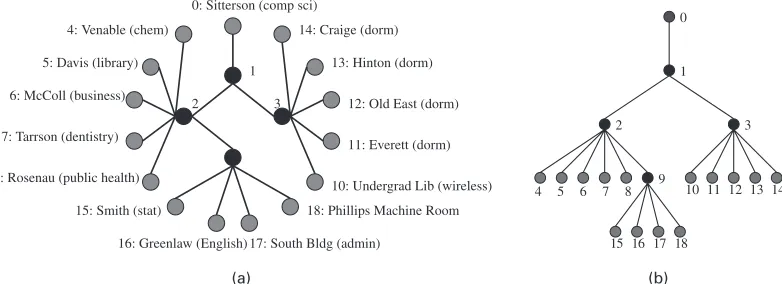
15 monitoring devices from Avaya Laboratories were deployed in a variety of buildings and on a range of capacity links through the UNC network. The locations included dormitories, libraries and various academic buildings. The links included large capacity gigabit links, smaller 100 Mbit links and one wireless link. Monitoring VOIP transmissions between these buildings allows us to examine traffic influenced by the physical conditions of the link and the demands of various groups of users. Fig. 1(a) gives the physical connectivity of the UNC network. Each of the nodes on the circle has a basic machine that can place a VOIP phone call to any of the other end points. The three nodes in the middle are part of the core (main routers) of the network. One of these internal nodes, the upper router linked to Sitterson Hall, also connects to the gateway that exchanges traffic with the rest of the Internet. The measured data consist of end-to-end delays and losses. We shall use data that were collected from this study to illustrate our methodology in Section 8.
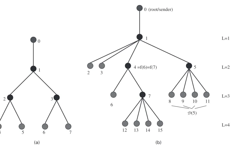
[image:2.485.46.437.471.613.2]Although the physical structure of a network can be arbitrary (Fig. 1(a)), the logical topology for the probing experiment can be represented more simply (Fig. 1(b)). We shall follow the com-mon practice in the literature and focus attention on logical topologies that can be described by trees:acyclic graphs with one vertex designated as the root(Fig. 2(b)). Formally, letT =.V,E/be a tree with node setVand link setE. The nodes follow a canonical numbering scheme, starting from the root node 0. All links will be named after the node at their terminus so, in Fig. 2, link
Fig. 2. (a) Three-layer, binary, symmetric tree and (b) general tree with notation
1 refers to the link connecting nodes 0 and 1. The parent of nodek∈V will be writtenf.k/. In a tree, all nodes have a parent except for the root node. Definefi.k/recursively as follows: fi.k/=f{fi−1.k/}, wheref1.k/=f.k/. Nodekis said to be in layerLiffL.k/=0. LetD.k/ denote the children of nodek, which is the collection of nodes whose parent isk. LetRdenote the set of leaf or receiver nodes, i.e. nodes with no children. Finally, an internal node is a node with both a parent and a set of children. Fig. 2(a) shows a simple binary tree with three layers. We shall use it later to illustrate some of the techniques.
Packets can be sent from a source to a destination by using two basic transmission protocols: a ‘unicast’ scheme that sends a packet from a source to one receiver at a time, and a ‘multicast’ scheme that sends a packet simultaneously to a set of specified receivers. In previous work, the term multicast experiment refers to the situation in which all the receiver nodes are probed simultaneously. We shall refer to it instead as an ‘omnicast’ probing experiment. The ‘flexicast’ experiments in Section 3 are also based on multicast transmission, although they do not involve sending the packet to all receivers in the network.
The estimation of loss rates based on active probing has been studied by many researchers (see Cácereset al.(1999), Xiet al.(2007) and references therein). Link delay tomography was first studied by Lo Prestiet al.(2002), who developed a heuristic estimator for omnicast exper-iments based on solving polynomial equations, which can be very inefficient. Liang and Yu (2003) developed a pseudolikelihood approach by considering all possible pairwise results from each individual full omnicast result. We shall compare these two techniques with our methods later in the paper. Shih and Hero (2003) presented an estimator that models link delay by using a point mass at zero and a finite mixture of Gaussian distributions.
end-to-end, path level data. Section 4 deals with maximum likelihood estimation using the EM algorithm and develops its computational and theoretical aspects. Alternative heuristic algo-rithms that are faster and scale well to larger networks are discussed in Section 5. An extensive numerical investigation of the procedures is also presented by using thens-2network simu-lation software. Finally, the methods are illustrated on real data that were collected from the UNC campus network.
2. Models and assumptions
Following Lo Presti et al. (2002) and Liang and Yu (2003), we shall consider nonparamet-ric estimation of the delay distributions by using a discrete distribution with a fixed, univer-sal bin size. Specifically, letXk be the delay that is accumulated on linkk, taking values in
the set {0,q, . . . ,bq}. Here q is the bin size and b is the maximum discrete delay (which is assumed to be common for all the links). Although this framework seems restrictive, it is use-ful for several reasons. First, experience with real network traffic data shows that behaviour tends to vary with the particular network being studied, so selecting a particular parametric family for modelling the link delay distribution is difficult. Moreover, the delay data typically exhibit bursty behaviour, in which case the tails of the distribution are of considerable inter-est. The discrete model makes no assumptions about where the mass is located, so the tails of heavy-tailed distributions can be estimated provided that we have a sufficient number of probes. The bin size can be chosen adaptively after the data have been collected. Smaller bin sizes can be used to estimate detailed information about the distribution. Large bin sizes can be used to obtain tail information. Examples of this will be discussed in the data analysis section.
Throughout the paper, we shall ignore losses or infinite delays. We can always estimate the loss rates and the finite delay distributions separately and combine the results to estimate the overall network behaviour. In addition, we make the assumption (which is common in the net-work tomography literature) that the packet delays are temporally independent and that the delay of a packet on a link is independent of the delay on the other links in the path. The assumption of temporal independence is reasonable as long as the interval between probes is sufficiently large. Temporal stationarity is reasonable as long as the probing period is sufficiently short to avoid major network changes. The adequacy of the spatial assumption will depend on the particular network being studied and whether there are other physical links connecting the nodes.
The data are collected by recording the total delay that a packet experiences as it travels from the root node to the receiver nodes. For example, in Fig. 2(b), probe packets would be sent from node 0 to various collections of nodes 2, 3, 6, 8, 9, 10, 11, 12, 13, 14 and 15 and the delays that are experienced along their corresponding paths would be recorded. Physically, each end-to-end delay is the sum of the individual link delays along the path. If a scheme has a collection ofk receivers, a single observation would be ak-tuple of delays.
LetP0,kdenote the path from node 0 to nodek, and let
Yk=
i∈P0,k Xi
be the cumulative delay accumulated from the root node to nodek. For example,Y3=X1+X3 in Fig. 2(b). The measurements that are obtained from a delay tomography experiment consist of cumulative delaysYr,r∈R. Letαk.i/=P.Xk=iq/, i=1, . . . ,b. Our objective is to estimate
In what follows, we shall use the notation αk=.αk.0/,αk.1/, . . . ,αk.b// and α=.α0,
α
1, . . . ,α|E|]/. Letπj,k.i/be the probability that the delay that is accumulated on path Pj,k
is equal toiunits. This is a function ofα.
3. Flexicast probing experiments
Although the omnicast probing experiment is easy to implement, it suffers from several disad-vantages. Suppose that there areRreceivers and the total number of possible bins associated with the path level delay distribution of theith receiver isBi. Then, the total number of possible
outcomes is of orderΠRi=1Bi, which can be a huge number. As we shall see later, the
computa-tional efficiency of most estimation methods depends on this number. As an example, let each link level delay distribution have the same number of bins:b=4. Further, suppose that we have a symmetric binary tree with five layers. Then, there areR=16 receivers andBi=19 for the path
level delay distributions of all the receivers, so the approximate number of possible outcomes is 2:8×10²⁰.
A second, perhaps more important, issue is the lack of flexibility as it involves probing the entire network each time. In practice, we are interested in monitoring the network over a period of time, and so we need a flexible scheme that allows us to probe different parts of the network with different degrees of intensity depending on where there are bottle-necks or quality-of-service problems. We consider a flexible class of probing experiments called ‘flexicast’ experi-ments to address these problems in the context of delay tomography.
Define ak-cast scheme as a scheme that sends probes from a receiver to a specified set of kreceiver nodes. For example, for the tree in Fig. 2(b),2,3is a two-cast (or bicast) scheme whereas6, 12, 13, 14, 15 is a five-cast scheme. A flexicast experimentC is a combination of k-cast schemesCj,j=1, . . . ,M, with possibly different values ofk, that allows us to estimate all
the link level parameters. Returning to Fig. 2, one flexicast experiment made up of a collection of bicast and unicast schemes isC={2,3,6, 12,13, 14,8, 9,10,11,15}. Another that uses largerk-casts isC={2,3,6, 12, 13, 14, 15,8, 9, 10, 11}.
A natural question is when will a flexicast experiment lead to identifiability? We provide below a necessary and sufficient condition. The proof is based on the idea that an individual k-cast probe can identify all the path distributions between branching nodes on its subtree. It suffices for the collection to be sufficiently rich in terms of subtrees that the individual links can be expressed as functions of paths from different schemes. We formalize this intuition in the following proposition. The proof is deferred to Appendix A.
Proposition 1.LetT be a general tree network, and suppose that its link delay distributions are discrete. LetCbe a collection ofk-cast schemesCj,j=1, . . . ,M. The link level delay distri-butions are identifiable if and only if
(a) for every internal nodes∈T\{0,R}there is at least onek-cast schemeCj∈C, withk >1,
such thatsis a branching node forCj, and
(b) every receiverr∈Ris covered by at least oneCj∈C.
and receiver nodes 2 and 3. Let the link level delay random variables beX1,X2andX3and the path level delay random variables at receiver nodes 2 and 3 beY2=X1+X2andY3=X1+X3. Suppose that theXis are independentN.μi, 1). Then, we cannot recover theμis from the joint
distribution ofY2andY3.
4. Maximum likelihood estimation
Active delay tomography is a large scale inverse problem. For example, consider the omnicast problem for the topology that is given in Fig. 2(b). Here we must use the 11-dimensional end-to-end measurements to estimate the 15 link delay distributions. The key is the dependence among the 11-dimensional data that is induced by the simultaneous probing. This dependence gives us additional information that allows us to deconvolve the path level delay into link level information. We consider maximum likelihood estimation first.
We need some additional notation. LetTCj be the subtree that is probed by schemeCj∈C, with node setVCj and link setECj. LetXCj={0, 1, . . . ,b}|ECj| be the set of all possible link delay combinations that could arise from this scheme. Eachx∈XCj is an|ECj|-tuple giving a possible link delay combination. Let the functiony.x,TCj/give the end-to-end delay arising in schemeCj from link outcomex∈XCj. Define the set of all possible end-to-end delays as
YCj={y.x,TCj/|x∈XCj}. LetγCj.y/=P.YCj=y/, the probabilities for the end-to-end experi-mental outcomes.
We illustrate this notation by using Fig. 2(b). Suppose that we probe the pair2,3. Letb=1 soXk∈{0, 1}. The link set isE2,3={1,2,3}. Assume that only a single probe packet is used for
this scheme, and it experiences link delays of 0, 1 and 1 on each link. We then havex=.0, 1, 1/ andy=.1, 1/. The probability of this link delay set is
P{X2,3=.0, 1, 1/}=α1.0/α2.1/α3.1/:
The probability of this end-to-end outcome is
P{Y2,3=.1, 1/}=α1.0/α2.1/α3.1/+α1.1/α2.0/α3.1/,
which is the sum of the probabilities for the link outcomes which can give rise to this end-to-end outcome.
4.1. EM algorithm
The discrete nonparametric distribution framework results in multinomial outcomes for path level data. Specifically, the observations consist of the number of times that we observe each individual outcomeyfrom the set of outcomesYCjfor a given scheme. Denote these counts as NyCj . Consider the likelihood equation
l.α;Y/= Cj∈C
y∈YCj
NyCjlog{γCj.y;α/}: .1/
The E-step can be broken into two parts. Assume that we have some parameter vector
α.q−1/. First, we compute the expected number of times that each link delay vectorxoccurred
as
NxCj.q/= P.X
Cj= x/.q/
P{YCj= y.x/}.q/N
Cj
y : .2/
Then, we use these values to compute the number of times that probes on linkkhad a delay of iunits as
Mk.q/,i = Cj∈C:k∈TCj
x∈XCj:xk=i
NxCj.q/: .3/
We also need to keep track ofmk, which is the total number of probes that crossed linkk.
The M-step is quite simple once the sufficient statistics have been imputed:
αk.i/.q/= 1 mkM
.q/
k,i: .4/
4.2. Partitioning
The computationally challenging aspect in our setting is to partition the observed end-to-end delays into the set of possible link delay combinations. These details are given next.
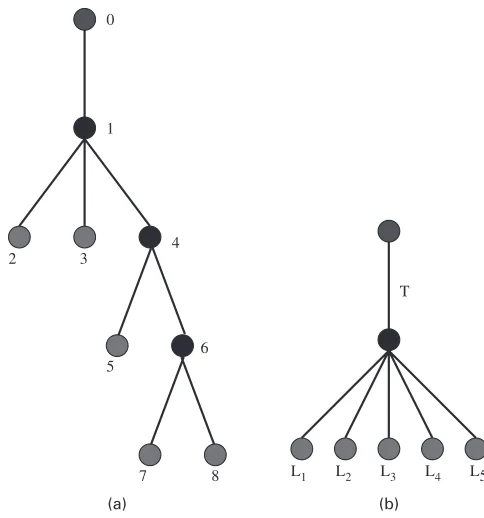
Consider Fig. 3(a). Suppose that this is the probing tree for a five-cast experiment and that the maximum link delay isb=2. Suppose further that a single probe results in the observed delay vectorY=.2 3 3 4 3/. We need to partition this end-to-end delay vector systematically into the complete list of all possible link delay vectors that give this result. We move from top to bottom, identifying possible delays for links starting at the top of the tree and moving downwards. We begin by listing possible link delays for the first link, between nodes 0 and 1, and leaving the rest of the delays as path delays. This amounts to imagining that the tree takes the form of the shrubthat is shown in Fig. 3(b), with each branch of the shrub hav-ing a maximum delay determined by band the number of links from node 1 to each of the receivers.
To obtain the lower bound of the possible delays for the first link, consider the minimum delay that is possible on this link that will give the observed values. The lower bound is the maximum of a set containing 0 and each observed value minus the maximum delay that could be obtained on its branch,Yr−grb, wheregris the number of links that are hidden in the branch
of the shrub connecting receiverrto the splitting node. For this example, the value is 1. The upper bound is simply the minimum ofband the set of observed values. Here the value is 2. This allows us to expand the observed delay into the set of link 1 delays and the remaining delays:
.2 3 3 4 3/→
1 1 2 2 3 2 2 0 1 1 2 1
: .5/
Fig. 3. Partitioning example: (a) probing subtree and (b) its corresponding shrub
1 1 2 2 3 2 2 0 1 1 2 1
→ ⎛ ⎜ ⎜ ⎜ ⎝
1 1 2 0 2 3 2 1 1 2 1 1 2 1 1 1 2 2 0 1 0 2 0 1 0 1 2 1 2 0 1 1 0 1 0
⎞ ⎟ ⎟ ⎟
⎠: .6/
Partitioning the second shrub gave us the range of values for links 4 and 5 leaving all the pairs comprising the last two columns. Each pair can be partitioned into the three component parts of this remaining shrub to give us the full partition for the observed delay on this tree:
⎛ ⎜ ⎜ ⎜ ⎝
1 1 2 0 2 3 2 1 1 2 1 1 2 1 1 1 2 2 0 1 0 2 0 1 0 1 2 1 2 0 1 1 0 1 0
⎞ ⎟ ⎟ ⎟ ⎠→ ⎛ ⎜ ⎜ ⎜ ⎜ ⎜ ⎜ ⎜ ⎜ ⎜ ⎝
1 1 2 0 2 1 2 1 1 1 2 0 2 2 1 0 1 1 2 1 1 0 2 1 1 1 2 1 1 1 1 0 1 1 2 2 0 0 1 0 2 0 1 0 1 0 2 1 2 0 1 0 1 1 1 0 2 0 1 1 0 0 1 0
⎞ ⎟ ⎟ ⎟ ⎟ ⎟ ⎟ ⎟ ⎟ ⎟ ⎠ : .7/
function is all that is required: it would partition the tree as if it were a shrub and then call itself to partition the subshrubs.
The algorithm for the general shrub withrreceivers is quite simple. LetY=.Y1, . . . ,Yr/be the
delay that is observed on the shrub. Further, lettbe the maximum delay that can be observed on the trunk and letlibe the maximum delay that can be observed on leafi. We have
a=max{0, max
i .Yi−li/}, .8/
z=min{t, min
i .Yi/} .9/
as the minimum and maximum possible values for the trunk delay. Thus, in one for-loop it is easy to make the expansion:
Y=.Y1, . . . ,Yr/→X=
⎛ ⎜ ⎜ ⎝
a Y1−a . . . Yr−a
a+1 Y1−.a+1/ . . . Yr−.a+1/
::
: ::: : :: ::: z Y1−z . . . Yr−z
⎞ ⎟ ⎟
⎠: .10/
4.3. EM complexity
To study the complexity of a single EM iteration, consider first a specifick-cast scheme. There are b|TCj|link delay outcomes for this probe. For each of these, there are|TCj|multiplications to compute the probability of the link delay outcome. For each outcome, there is also a single addi-tion to tally up the end-to-end probabilities and a single division to compute the condiaddi-tional probability of each outcome given the end-to-end outcome. Finally, there are|TCj|additions to tally up the sufficient statistics. Overall, this gives usO.b|TCj|/operations. The largest subtree sets the complexity for the E-step atO.b|TClarge|/whereClargeis the experiment on the subtree with the most links. The M-step is trivial, consisting of|Eb|divisions.
There are a few things to note. First, mixtures of bicast (k=2) and unicast schemes offer the best complexity while meeting the identifiability conditions. Additionally, they scale better than k-casts with larger values ofk. In particular, an omnicast scheme does not scale well.
If the tree grows in size but not in depth, then the bicast schemes should scale well because this will simply result in more bicast schemes rather than more complicated bicast schemes. This property does not hold for omnicast schemes which have complexityO.b|E|/.
Also of note, the complexity that is stated here is the extreme worst case based on observing every possible delay combination from every probing experiment. In practice, both the parti-tioning and the estimation consider only the observed delays which will significantly reduce the average case complexity.
Unfortunately, the EM algorithm does not scale well as the tree becomes deeper for any k-cast scheme. For such topologies, we explore alternative fast estimators in a later section. Note, however, that the EM algorithm can be made computationally more efficient through parallelization. Note that the E-step involves computing a sum that ranges first over the schemes and then over the outcomes for that experiment. This sum can be broken down into component pieces which can be computed simultaneously and combined.
4.4. Numerical investigation of EM algorithm
be estimated quickly and still provide enough information to detect anomalies in the network. However, we can only obtain a smaller tree by lumping several links together and eliminating some of the receivers.
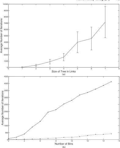
Consider first the effect of the tree size, in terms of both number of links and layers. We start with a two-layer symmetric binary tree so that there is a total of three links. Then, we add two children at a time. So the five-link tree corresponds to adding two children to one of the receiver nodes. The seven-link tree adds two children to the other receiver nodes (so this is just a three-layer symmetric binary tree). We proceed in this manner until we obtain the four-layer symmetric binary tree with 15 links (see thex-axis of Fig. 4(a)). The remaining model components are held fixed. In particular, each link has a five-bin uniform delay dis-tribution that is chosen because it provides maximum entropy; thus it is the most difficult to resolve. We use a flexicast experiment that is a minimal set of bicast schemes that satisfy the identifiability conditions. Some additional studies indicated that convergence for the EM algo-rithm does not seem to depend greatly on the number of probes that are used. Hence, in these investigations, each bicast scheme used 1000 probes for each link in its subtree. For each tree size, 50 sets of data were generated and used for estimation. The convergence criterion was a change in the log-likelihood of less than 10−4. Fig. 4(a) shows the number of iterations that are required for convergence for each data set. The average number of iterations for each size is plotted with standard deviation error bars. This suggests that the average number of itera-tions seems to be increasing at a rate that is faster than linear (perhaps exponential) with the number of links. This is a further indication that the EM algorithm does not scale well to larger networks.
Next, consider the effect of the number of bins in each link with uniform delay distributions. The number of bins on each link was varied from 2 to 15. We considered both two-layer and three-layer binary symmetric trees with three and seven links respectively. Again, a minimal bicast experiment with 1000 probes per scheme was used. The results for both trees are shown in Fig. 4(b). In this scenario, the average number of iterations seems to grow approximately linearly with the number of bins on each link. This is an important observation that we shall exploit later in developing a faster algorithm.
4.5. Asymptotic properties of the maximum likelihood estimator
Given the multinomial nature of the underlyingk-cast schemes, the asymptotic properties of the maximum likelihood estimator (MLE) mostly follow from general principles. The difference arises because the flexicast experiments imply that individual probes are not independent and identically distributed. The proposition below establishes that the Fisher information matrix is positive definite at the true valueα0. Thus, the likelihood has a unique maximum in a local neighbourhood of the true valueα0.
Proposition 2.The Fisher information matrixI.α0/for the MLE based on end-to-end quan-tized measurements from a flexicast experimentCis finite and positive definite.
The proof can be found in Lawrence (2005). The main idea is to treat the Fisher information as the covariance of the score function and then to consider various hypothetical data sets to establish that it must be positive definite.
Proposition 3.LetnCj=n→λCjasn→∞with 0<λCj<1 forj=1, . . . ,M. Then,αMLE→ α0, almost surely, and√n.αMLE− α0/⇒Z, whereZ∼N{0,I−1.α/}.
Fig. 4. (a) Number of iterationsversustree size and (b) number of iterationsversusbin size for two- ( . . . .) and three- ( ) layer trees
5. Faster, heuristic, algorithms
5.1. Grafting
Fig. 5. Peeling is the process of using a known path distribution and the known distribution for one end of the path to solve for the distribution of the other end
path distribution and a known distribution from one end of that path to solve for the distribution on the other end (see the proof of proposition 1). In essence, grafting treats eachk-cast scheme as an omnicast experiment on the probing subtree. It uses an EM algorithm to solve for the MLE of the logical links on this subtree and then uses peeling to obtain estimates for individ-ual links. For collections of bicast and unicast schemes, this technique scales very well because the EM algorithm is applied to a series of three-link, two-layer trees. Thus the complexity is a cubic polynomial in the number of bins, which is a vast improvement over the standard MLE complexity. On the basis of the investigations that were discussed previously, increasing the number of bins on the links increases the average number of iterations approximately linearly whereas adding links tends to increase the required iterations exponentially. This local scheme takes advantage of this fact by trading links for bins.
We shall explain the details by using a flexicast experiment with just bicast and unicast schemes. First, consider a bicast scheme and the corresponding subtree. Let the trunk havetlinks and the two branches havel1andl2links. The subtree has just three logical links with varying numbers of bins on each: the trunk hastb+1 bins and the branches havel1b+1 andl2b+1 bins. We apply the EM algorithm to this logical subtree and solve for its MLE. This is done for all the bicast schemes. This gives the estimates for the trunks and branches of all the bicast subtrees.
Individual links can be now be obtained in one of several ways. Consider first the simple peeling from the proof of proposition 1. This is straightforward and non-iterative although not very statistically efficient as only some of the bin probabilities from each known distribution are used in computing the unknown distribution. At least one pair must split at node 1, so at least one of the local MLEs must give us an estimate for link 1. Now, at least one scheme gives us the local MLE for the path from the root node to every child of node 1. So the individual links up to these points can be identified through peeling. This process continues down the tree, identifying each link. The receivers that are covered by bicast experiments can be identified as the branches in a subtree or by peeling from the branches. The receivers that are covered by only unicast experiments can also be identified by peeling.
We now propose a more sophisticated peeling mechanism. This is a fixed point type of algo-rithm that arises from postulating an EM algoalgo-rithm for imaginary data. Imagine that we sendn probes across the path. Form data by settingnd=nπ0,2.d/. The data are counts of the number
of times that delayd was observed on the path for all possibled. In the E-step, we want to computeMi, the expected number of times that delayiwas seen on the unknown link. After the
qth iteration, this is given by
Mi.q+1/=b
j=0
α.q/
2 .i/α1.j/
π.q/
0,2.i+j/
ni+j, .11/
whereπ.q/0,2is updated with each update ofα.q/2 . Note that this is not the quantity that was used to generate the data. Since we obtain our estimates by dividingMibyn, we obtain
α2.i/.q+1/=b
j=0
α.q/
2 .i/α1.j/
π.q/
0,2.i+j/
This equation is no longer based on our imaginary data. It is run untilα2approaches its fixed point. Note that this fixed point algorithm is simply an EM algorithm for computing one link level distribution from the path level and other link level distributions and meets standard condi-tions for convergence. Unlike the simple method, this peeling function uses all of the information from the two known distributions.
The peeling method can lead to multiple estimates for some links. The easiest way to address this problem is to combine them, using either a simple average or a weighted average. For the latter, if we have two estimates ofα1from experiments C1 andC2, we can combine them as follows to obtain
˜ α1=n
C1αC1+nC2αC2
nC1+nC2 : .13/
It can be shown that the grafting algorithm yields estimators that are consistent and asymp-totically normal. The computation of the asymptotic variance is complicated and the simplest way to compute the variance is to use bootstrap or other resampling methods.
5.2. A comparison of the various estimators 5.2.1. Other estimators in the literature
Two other estimation procedures have been proposed in the literature for the delay tomography problem. Both are based on omnicast probing and rely on the same modelling assumptions as those presented here: discrete delay with temporal and spatial independence. The first, which was discussed by Lo Prestiet al.(2002), depends on solving polynomials. At some linkk, the estimator uses the data from the subtree rooted at the link to create a polynomial for each unit of delay,i. The degree of the polynomial is|D.k/|. The second root of this polynomial gives us the cumulative probability of delayion linkk. The principal drawback of this estimator is that it does not use all of the information that is available. End-to-end delays that are larger than the largest allowable link delay are ignored. Additionally, the nature of the estimator allows inappropriate results from the polynomial solution such as negative values or values that are greater than 1.
The estimator by Liang and Yu (2003) is based on a pseudolikelihood approach. The com-plexity of the omnicast experiment is reduced by looking at just bicast projections—all pairwise combinations—and using a pseudolikelihood that treats them as independent. For example, the network in Fig. 2(b) has 11 receivers, so the omnicast experiment results in 11-dimensional delay observations. There are 55 possible pairs of receivers, so the pseudolikelihood scheme treats all the possible pairs of delays as 55 independent bicast observations. The motivating idea is that processing the data as pairs is computationally much more efficient than processing the omnicast data. This can be justified if the gain in computational speed offsets the loss in statistical efficiency.
5.2.2. Computational efficiency
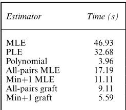
Table 1. Three-layer tree com-parison: average computing time
Estimator Time (s)
MLE 46.93
PLE 32.68
Polynomial 3.96
All-pairs MLE 17.19
Min+1 MLE 11.11
All-pairs graft 9.11
Min+1 graft 5.59
just bicast schemes. To see this, consider the three-layer, binary, symmetric tree in Fig. 2(a). The minimal bicast experiment is {4, 5,5, 6,6, 7}. This experiment is unbalanced as receiver links 4 and 7 are covered only once whereas links 5 and 6 are covered twice. A more balanced approach is obtained by adding pair 4, 7. This ensures that each link on a particular layer of a binary, symmetric tree is covered by the same number of experiments. We refer to such experiments as min+1 flexicast experiments.
In addition to the MLEs, we also consider the pseudolikelihood estimator (PLE), the poly-nomial estimator from Lo Prestiet al.(2002) and grafting for all-pairs bicast and min+1 bicast experiments. All the estimators were implemented by using MATLAB with the combinatorial partitioning components of the likelihood-based methods written in C. The link delays follow a five-bin truncated geometric distribution. The parameters of the distributions were varied in a manner to keep the situations realistic: the interior links have high probability of 0 as com-pared with edge links to simulate the difference between internal links with large bandwidth and smaller local links. The comparisons of efficiency were based on 100 simulated data sets and are shown in Table 1.
The polynomial estimator is, of course, the fastest. This is partially driven by the fact that it is solving quadratic equations in this example (binary tree) and the formulae for the estim-ates are obtained explicitly. The effect of having a large number of children on the polynomial estimator will be investigated later. We shall also see later that this algorithm can be consid-erably inefficient in a statistical sense. As is to be expected, the PLE is faster than the MLE based on the full EM algorithm; however, it does not gain as much over the MLE as does the pure bicast algorithm. The all-pairs bicast is more than twice as fast as the likelihood-based multicast estimators, whereas the PLE does not seem to benefit from an order of magnitude gain.
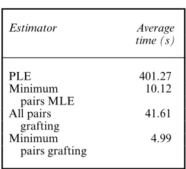
Table 2. Computational speeds of estimators applied to data from Fig. 2(b)
Estimator Average time (s)
PLE 401.27
Minimum 10.12
pairs MLE
All pairs 41.61
grafting
Minimum 4.99
[image:15.485.177.314.267.372.2]pairs grafting
Table 3. Comparison of computa-tion time for grafting and the polyno-mial estimator on shrubs with varying numbers of children
Number of Times (s) for the children following estimators
Grafting Polynomial
2 0.48 1.02
6 0.84 1.08
10 0.99 1.13
with minimum pairs is extremely fast, comparable in speed with the time that is achieved by the polynomial estimator on the simpler tree that was discussed previously.
5.2.2.2. Shrub comparison. Here we investigate only the two fastest estimators: the grafting procedure with minimum bicast pairs and the polynomial estimator. We study a set of simple cases: shrubs with increasing numbers of children to see how the performance varies. For each configuration, we generated 1000 data sets from truncated geometric distributions on each link. Table 3 lists the average computation times for shrubs with two, six and 10 children. The grafting procedure is uniformly faster on this test, even when it must combine information from five trees in the 10-child example. The polynomial estimator performs at its best on small trees with small numbers of bins. However, when the true bin probability is small, we found that it can lead to negative estimates in a significant number of cases.
5.2.3. Statistical efficiency
We also note that it is difficult to compare the statistical efficiencies of estimates that are based on bicast or other flexicast experiments with those that are based on an omnicast experiment as they are not on an equal footing. If the total number of probes is fixed, the total amount of traffic expected is different for omnicast and flexicast experiments. Even if we fix the total amount of expected traffic on all links under the schemes, different links will have different expected num-bers of probes. It is not possible to make the expected number of probes in each link be the same under the different schemes. Moreover, omnicast experiments contain information about all higher order moments whereas the flexicast experiments are designed to sacrifice the higher order moments to reduce data complexity.
[image:16.485.53.306.279.607.2]To keep the comparisons meaningful, we shall examine the efficiencies of estimation meth-ods based on omnicast and bicast experiments separately. The comparisons here are based on a three-layer symmetric binary tree. The link delay distributions were chosen to be truncated geometric with five bins.
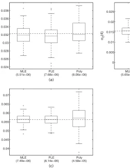
[image:16.485.250.439.281.439.2]Fig. 6 shows the performance of the full EM-based MLE, PLE and the polynomial estimator for the last bin for three links:α1.4/,α2.4/and α4.4/. The size of the omnicast experiment was 20 000 total probes. Recall thatα1is the first link on the tree whereasα4corresponds to one of the receiver nodes. Fig. 6 suggests that the bias is small (medians close to the true values).
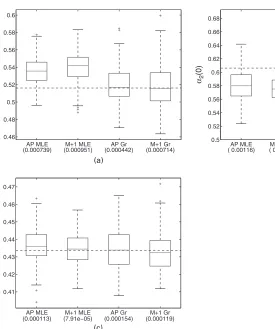
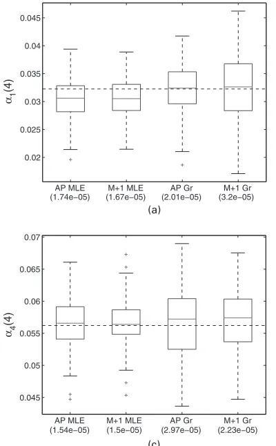
Fig. 7. Box plots of the estimates for (a)α1.0/, (b)α2.0/and (c)α4.0/for four bicast-based estimators (mean-squared errors are given in parentheses)
The performance of the PLE is close to that of the MLE on links 1 and 4 with interquartile range ratios of 1.01 and 1.06. The performance on the interior link is somewhat worse with an interquartile range ratio of 1.38. This conclusion seems to be true in general; i.e. the relative performance of the PLE grows worse as we move to the interior of the tree. So we would expect the performance to be poor for internal nodes in the middle of a large tree with many layers. The polynomial estimator, in contrast, is considerably less efficient in all three cases with interquartile range ratios of 1.36, 3.18 and 2.47. The mean-squared error (which is shown on the plots beneath the labels) tells a similar story. For the PLE it is 1.39, 1.72 and 1.09 times as large as that for the MLE and for the polynomial estimator it is 1.46, 7.49 and 6.11 times as large as that for the MLE. We also compared the performance of the estimators for other bins and links. In general, the performance of the polynomial estimator is quite good for the first link (α1) but becomes progressively worse as we move deeper down the tree. This is because the polynomial estimator uses much of the data in estimating the first link but uses increasingly less data as we move down.
For the bicast-based estimators, we considered two different experiments:
Fig. 8. Box plots of the estimates for (a)α1.4/, (b)α2.4/and (c)α4.4/for four bicast-based estimators (mean-squared errors are given in parentheses)
The estimators include the all-pairs MLE, all-pairs grafting, min+1 MLE, and min+1 graft-ing. The comparisons of the estimators for the first and last bins are shown in Figs 7 and 8 respectively. In terms of precision, the min+1 MLE is very comparable with the all-pairs MLE except for estimatingα2.4/. Forα4.4/, it is actually slightly better. This can be explained by the fact that the min+1 experiment allocates more probes for a scheme,4, 5, that isolates link 4, thereby giving us a more precise estimate for this link. The grafting algorithms do slightly worse than the MLEs. For the all-pairs experiment, the interquartile range ratios of the grafting estimates to the MLEs for the zero bin on links 1, 2 and 4 are 1.27, 1.02 and 1.41. For the four bins they are 1.23, 2.16 and 1.56. For the min+1 experiment, the interquartile range ratios for the zero bins on links 1, 2 and 4 are 1.44, 1.65 and 1.19. For the four bins they are 1.80, 1.44 and 1.74. In general the less precise algorithms do not perform as well in the interior of the tree at the tails of the distributions.
6. Optimal allocation of probes
We now turn to an important issue in designing flexicast experiments, i.e. how to allocate the number of probes optimally among the various schemes within a flexicast experiment. The ques-tion of interest is the following: given a fixed budget of probes, how should they be allocated among the various flexicast schemes?
It turns out that the optimal allocations depend on the values of the unknown delay distri-butions and the tree topology. This is calledlocal optimalityin the design literature (Chernoff, 1953). We describe results from a limited study based on binary symmetric trees and bicast schemes to provide some insights and suggest how one could go about studying the problem in general. A comprehensive study of this problem is part of on-going work.
We conduct our study on a three-layer binary symmetric tree (Fig. 2(a)). For each link delay distribution, we use a geometric distribution truncated to five bins. On the basis of our experience with real data and the network simulator, the truncated geometric distribution is a reasonable choice with its large mass at 0 and decaying tails. We let the parameter of the distributions range fromp=0:1 top=0:9 with a step size of 0:1. This range allows us to consider very good links with light tails (p=0:9) and more congested links with heavier tails (p=0:1).
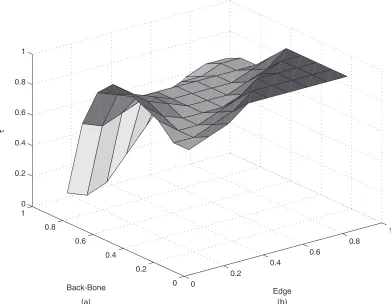
We use the following bicast experiment:C={4, 5,6, 7,5, 6,4, 7}. Note that the last two schemes split at node 1 whereas the first two schemes split at a lower level. We view links 1, 4, 5, 6 and 7 as edge links whereas links 2 and 3 will be considered internal or back-bone links. Links of the same type (edge and back-bone) will have the same distribution. On the basis of this symmetry, the optimal proportion of probes that are sent to schemes4, 5and6, 7should be equal; likewise for schemes5, 6and4, 7. Letτrefer to the total proportion of probes that are sent to the first group; then the second group will receive a proportion 1−τ. The design problem is to identify the optimal value ofτ.
The criterion that we use here isD-optimality, which is commonly used in the experimental design literature. Specifically, the optimal value ofτis obtained by maximizing the determin-ant of the Fisher information matrix. As noted before, this value depends on the unknown parameters of the delay distributions, in addition to the tree topology. This is referred to as localD-optimality.
First, we consider the optimalτfor the situation in which all the link level distributions are identical. Interestingly, the optimal value ofτis constant (around 0.75) aspranges from 0:1 to about 0:8 and then decreases slightly to about 0:7 aspincreases to 0:9. On the basis of this, the bicast pairs4, 5and6, 7, which split at a lower level in the tree, should receive about 35–37% of the probes each whereas pairs5, 6and4, 7, which split at a higher level, should receive only about 12–15% of the probes. Note that the pairs that split at the lower level provide the most information for estimating the receiver links. Further, the total number of probes at each link varies: under the above optimal setting, all the probes pass through the link at the top layer, links in layer 2 (the ‘back-bone’ links) each see about three-quarters of the probes, and those at layer 3 (receiver links) each see only a quarter of the probes.
Fig. 9. (a) Optimal allocation of probes with all links the same and (b) optimal allocation of probes with interior links the same and edge links the same
receive a larger proportion of the probes. This is probably due to the higher congestion on link 1 as compared with the back-bone links. Probes splitting at node 1 help to provide a good estimate of link 1, which is important in this case for sorting out the links below it.
The above results provide some limited insights into the optimal allocation issue. As noted before, the optimal results depend on the unknown delay distributions, so we cannot obtain universally optimal results for all distributions. In practice, we can take various approaches in achieving efficient (or close to efficient) probe allocations. The simplest is to use prior knowl-edge based on historical information and to treat it as the truth. A better alternative that uses prior information more formally is the use of Bayesian optimal design techniques (see, for example, Chaloner and Verdinelli (1995)). However, this is a complex, non-linear optimal design problem. Perhaps the most practical alternative is to use a two-stage experimentation where the estimates from the first stage are used to obtain the optimal estimates for the second-stage probing.
7. Simulation studies
(a) under the stochastic model assumptions in Section 2 and (b) using thens-2network simulator.
7.1. Model-based simulation
Our simulation studies showed that, if the true link level distributions are discrete, the MLE as well as grafting methods can recover the link level estimates well without any bias. When the true distributions are continuous, however, the binning seems to introduce some bias. The problem arises from the fact that the end-to-end data are grouped into bins, so we have discretized sums instead of sums of discrete values from each link. The extent of the bias depends on the bin size, the link and other variables.
[image:21.485.45.441.259.596.2]To develop some insights, we considered a three-layer symmetric binary tree (Fig. 2(a)) and focused on the MLE for a minimum bicast experiment. Each link distribution was taken to be a mixture of exponentials with mean 1 and point mass at 0. The point mass, corresponding to no delay, is common in many real situations. Various bin sizes and point mass probabilities were considered in the study. Fig. 10 show the results from links 1, 2 and 4 (link 3 has the same
Fig. 11. Observed () and estimated ( ) delays for links (a) 1 and (b) 2 of thens-2example
behaviour as 2 and links 5, 6 and 7 have the same behaviour as link 4) with a bin size ofq=0:25 and a point mass with probabilityp=0:2.
24% and 9% respectively. For a bin size ofq=4, the corresponding underestimates reduce to 8%, 6% and 4%. Note also from Fig. 10 that the bias is greatest for the receiver node (link 4) and decreases as we go up to the source node.
The effect of this bias on the other bins is much smaller. For the most part, the bias at the zero bin seems to be spread across the rest of the distribution. The estimate at bin 1 seems to compensate somewhat more than the other bins. There is also some compensation across links; the zero bin for link 1 is overestimated whereas the zero bins for other links are underestimated. We are currently exploring some methods for correcting this bias.
7.2. Network simulation
We now examine the performance of the proposed estimators in a realistic network environment by using thens-2(Information Sciences Institute, 2004) simulation package. This allows us to construct any topology, to generate traffic and to transmit packets by using a real network protocol. It gives users control over the hardware and software aspects of a network including bandwidth, propagation delay, traffic volume and traffic protocol. We constructed the topology that was shown in Fig. 1 to mimic the UNC network. For links between core routers, we used 500 Mbit links and, for links to end points, we used 50 Mbit links. Background traffic on the core links consists of 27 transmission control protocol connections and five user datagram protocol connections. Transmission control protocol connections acknowledge reception of packets by the receiver. Lost packets are retransmitted by the sender and result in a slower rate of transmis-sion. Therefore, transmission control protocol connections are responsive to congestion. User datagram protocol connections do not have any of these features and continue to send packets at a constant rate, thus being unresponsive to patterns of congestion. On the edge links, the background consists of six transmission control protocol connections and one user datagram protocol connection. The probe traffic consists of 40-bit user datagram protocol packets using the multicast protocol.
Every tenth of a second, the probing mechanism selects a scheme at random from C=
{4, 5,6, 7,8, 10,11, 12,13, 14,15, 16,17, 18}and sends a packet to its receivers. Prob-ing lasts for 700 s, resultProb-ing in about 1000 packets sent to each pair. This is approximately the length of a session that we would use for monitoring a real network. The end-to-end delays are discretized by using a bin size ofq=0:000 05 s. This is an extremely fine scale, resulting in a maximum link delay setting ofb=155. Furthermore, thens-2package allows us to record the true link delays and hence to obtain directly the link delay distributions for verification.
Figs 11 and 12 show the fitted distributions along with the observed distributions for selected links. We see the effect of the bias from binning that was discussed in the last section. Aside from this, the estimation procedure does a very good job of capturing the distribution despite a violation of the temporal and spatial independence assumptions in the model. The results show that the estimation procedure performs well in a real network setting.
8. Application to the University of North Carolina campus network data
Fig. 12. Observed () and estimated ( ) delays for links (a) 6, (b) 11 and (c) 15 of thens-2example
The data were collected by using a tool that was designed by Avaya Laboratories for testing a network’s readiness for VOIP. There are two parts to the tool. First, there are the monitoring devices: computers deployed throughout the network with the capability of exchanging VOIP style traffic. These devices run an operating system that allows them to measure accurately the time at which packets are sent and received. The machines collect these time stamps and report them back to the second part of the system: the collection software. This software remotely con-trols the devices and determines all the features of each call, such as source–destination devices, start time, duration and protocol, which includes the interpacket time intervals. The software collects the time stamps when the calls are finished and processes them. The processing consists of adjusting the time stamps to account for the difference between the machines’ clocks, and then calculating the one-way end-to-end delays.
Fig. 13. Probability of a large delay on each link throughout the day: (a) Sitterson; (b), (c) core to core; (d) Venable; (e) Davis; (f) McColl; (g) Tarrson; (h) Rosenau; (i) core to core; (j) university library; (k) Everett; (l) Old East; (m) Hinton; (n) Craige; (o) Smith; (p) Greenlaw; (q) South; (r) Phillips
to 1. Each probing session consisted of two passes through the pairs in the order presented. On each pass, each pair was probed for 50 s. Thus, we have 1000 probes for each pair during each monitoring session. Maximum likelihood estimation was used to deconvolve the link distributions.
In this section, we present results that are related only to discovering links that have signifi-cant probabilities of large delays. For this reason, we used a bin size ofq=0:0002 s. Above this threshold, delays can become detrimental to the quality of calls. We expect that most links in this network would have distributions with most of the mass on the zero bin. None-the-less, a mass as low as 0.01 on the rest of the delays could prove troublesome.
Fig. 14. Delay distribution at 12.00 p.m. and 10.00 p.m. for (a) Davis Library, (b) South Building and (c) Hinton Dormitory
spike is evident on link 9 which is a larger core-to-core router. The dormitory links show more consistent traffic throughout the entire day with some elevated delays in the later evening. Links that show 1% or more large delays would probably require an upgrade to be able to handle the increased load that is placed on them by VOIP, which uses a more aggressive protocol than the prevalent transmission control protocol traffic. Several receiver links already show close to 5% large delays without a strong VOIP presence. Even the large link 9 seems to be problematic as it needs to perform almost flawlessly to handle considerably more traffic than the receiver links.
To look at some aspects of the analysis in more detail, we solved the inverse problem using a bin size ofq=0:000 02 s for the time periods 12.00 p.m. and 10.00 p.m. This gave us 10 times the resolution of the above analysis. Further, it allowed us to break down the previous analysis to see where the delays fall within the smallest bin. Fig. 14 shows the first 20 bins of these detailed results for Davis Library, South Building and Hinton Dormitory. The first thing to note is that most of the mass is still on the lowest bins so the vast majority of packets experience very little delay. Both Davis Library and South Building exhibit a strong diurnal effect. Unlike the dormitory, the traffic in these buildings dies off late at night.
support-ing the VOIP application. From our point of view, the results are qualitatively consistent with the overall behaviour that is to be expected for this network. This serves as a validation of the techniques that were studied here, from both statistical and implementation perspectives.
9. Concluding remarks
We have introduced a flexible class of probing experiments for active network tomography and studied the properties of several methods for estimating the link level delay distributions of computer and communications networks. Both simulation and real data were used to illustrate the usefulness of the methodology. The use of the full EM algorithm is practical for small to moderate trees, especially with minimum identifiable flexicast experiments (bicast and unicast schemes). With larger networks, the grafting algorithm that was proposed in the paper provides a practical alternative. The fast algorithm is especially useful for monitoring the networks to detect degradation in quality of service and to localize the problem quickly to links or small regions of the network. We are currently studying monitoring and diagnostic procedures for this problem.
We have followed the literature in the area in making some simplifying assumptions. For example, the logical topology of the network has been assumed to be single source, known and fixed. Extensions to multisource topologies, although conceptually straightforward, neverthe-less introduce technical challenges that are currently under investigation. Further, in practice, the network’s topology can be to a certain degree unknown or changing periodically. There is on-going work in the network engineering literature to address these topics. The assump-tion of spatiotemporal staassump-tionarity is also commonly made in this area. As we have noted, the temporal stationarity assumption is not critical as the time between probes is of the order of milliseconds. The spatial assumption is more problematic although more realistic models can be developed only in the context of specific real networks. Additional work is also required to assess the performance of the methods for larger networks. We note, however, that even if the actual network is large, one typically aggregates many of the links and focuses on a smaller topology for studying network performance.
Acknowledgements
The authors thank the Joint Editor, the Associate Editor and two referees for useful comments and suggestions. The paper is part of the first author’s doctoral dissertation. The research was supported in part by National Science Foundation grants IIS-9988095, CCR-0325571, DMS-0204247 and DMS-0505535. The authors are grateful to Jim Landwehr, Lorraine Denby and Jean Meloche of Avaya Laboratories for making their ExpertNet tool available for VOIP data collection and for many useful discussions on network monitoring, Yinghan Yang for assis-tance with data collection, Jim Gogan and his team from the Information Technology Division at UNC for their technical support in deploying the ExpertNet tool on their campus network, for troubleshooting hardware problems and for providing information about the structure and topology of the network, Don Smith of the Computer Science Department at UNC for helping us to establish the collaboration with the UNC information technology group and Steve Marron for many helpful comments during the course of this research.
Appendix A: Proof of proposition 1
identifies all the distributions on the paths between source, branching nodes and receivers of its subtrees. We can then show that the above conditions guarantee that we have enough subtrees to solve for every link delay distribution. The proof of necessity will proceed by contradiction.
For omnicast probing, we consider two cases.
(a) Case 1—receiver node k—consider all omnicast probes that result in zero delay on all remaining receivers exceptk. This set of probes allows us to estimateαk as these probes consist of direct observations from linkk.
(b) Case 2—internal node k—we proceed by induction. Suppose that we have identified the distributions for all links that are descendants ofk. LetR.k/represent the receivers that are descended fromk. Consider probes that result in zero delay on all nodes except those inR.k/which all experiencei delay. Letγk.i/be the probability that eachr∈R.k/has an end-to-end delay ofi. From this, we can estimateγk.i/for eachi. Since we have estimates of link delay distributions of the descendants ofk, we can now estimateαk.
This proof implies that a singlek-cast scheme will identify the following distributions: the path between the source and the first splitting node, the paths between any two splitting nodes and the paths between a splitting node and a receiver. Now we focus on a collection of flexicast schemes. Here we consider three cases.
(a) Case 1: there is somek-cast schemeCjin which branching occurs at node 1, the only child of the root node. Based on the omnicast identifiability proof, this experiment identifies the delay distribution for link 1,α1.
(b) Case 2: letsbe some internal node. Assume that we have identified all the delay distributions for linksk∈P0,f.s/. There is a schemeCjfor which branching occurs at nodes. This scheme identifies the path level distributionπ0,s. We can constructπ0,f.s/and solve forαs:
αs.0/=π0,s.0/=π0,f.s/,
αs.d/= 1
π0,f.s/.0/
π0,s.d/− d−1
δ=max.0,d−Bf.s//
αs.δ/π0,f.s/.d−δ/
, ∀d=1, . . . ,b,
whereBf.s/is the maximum delay up to this node. We call this solution peeling since we are peeling the unknown distribution from the path level distributions. It can be used more generally and can take other functional forms.
(c) Case 3: letrbe some receiver node. Assume that we have identified all the delay distributions for linksk∈P0,f.r/. There is some schemeCjwhich probes receiverr. From this, we can estimate the path probabilityπ0,r. We can constructπ0,f.r/and use peeling to obtainαr.
It is easy to see the necessity of covering all the receivers: if we do not probe a receiver, we can never estimate its link delay distribution. To see the necessity of branching at each internal node, consider a col-lection of schemes in which branching occurs at all internal nodes except some nodes. Each linkd∈D.s/ will always occur as part of a logical link that also includes links. We will be able to obtain estimates for
πf.s/,d for eachd∈D.s/but we shall have no information with which to peel the two apart. In essence, these estimates are like unicast measurements which are not sufficient for estimation.
References
Cáceres, R., Duffield, N. G., Horowitz, J. and Towsley, D. F. (1999) Multicast-based inference of network-internal loss characteristics.IEEE Trans. Inform. Theory,45, 2462–2480.
Cao, J., Davis, D., Vander Wiel, S. and Yu, B. (2000) Time-varying network tomography: router link data.J. Am. Statist. Ass.,95, 1063–1075.
Castro, R., Coates, M., Liang, G., Nowak, R. and Yu, B. (2004) Network tomography: recent developments. Statist. Sci.,19, 499–517.
Chaloner, K. and Verdinelli, I. (1995) Bayesian experimental design: a review.Statist. Sci.,10, 273–304. Chernoff, H. (1953) Locally optimal designs for estimating parameters.Ann. Math. Statist.,24, 586–602. Information Sciences Institute (2004)The Network Simulator. Marina del Rey: Information Sciences Institute.
(Available fromhttp://www.isi.edu/nsnam/ns/.)
Lawrence, E. (2005) Flexicast network delay tomography.PhD Thesis. University of Michigan, Ann Arbor. Liang, G. and Yu, B. (2003) Maximum pseudo likelihood estimation in network tomography.IEEE Trans. Signal
Lo Presti, F., Duffield, N. G., Horowitz, J. and Towsley, D. (2002) Multicast-based inference of network-internal delay distributions.IEEE Trans. Netwrkng,10, 761–775.
Shih, M.-F. and Hero, A. O. (2003) Unicast-based inference of network link delay distributions with finite mixture models.IEEE Trans. Signal Process.,51, 2219–2228.
Tebaldi, C. and West, M. (1998) Bayesian inference on network traffic using link count data.J. Am. Statist. Ass., 93, 557–573.
Vardi, Y. (1996) Network tomography: estimating source-destination traffic intensities from link data.J. Am. Statist. Ass.,91, 365–377.
Xi, B., Michailidis, G. and Nair, V. N. (2007) Estimating network loss rates using active tomography.J. Am. Statist. Ass., to be published.