On nonlinear matrix equations \(X\pm\sum {i=1}^{m}A {i}^{*}X^{ n {i}}A {i}=I\)

(1)

R E S E A R C H

Open Access

On nonlinear matrix equations

X

±

m

_i

_=

A

∗

_i

X

–

n

i

A

i

=

I

Asmaa M Al-Dubiban

*

*_{Correspondence:}

[email protected] Faculty of Science and Arts, Qassim University, Buraydah, Kingdom of Saudi Arabia

Abstract

We study the nonlinear matrix equationsX+m_i=1A∗_iX–ni_A

i=Iand X–m_i=1A∗_iX–ni_A

i=I, whereniare positive integers fori= 1, 2,. . .,m. The iterative

algorithms for obtaining positive definite solutions for these equations are proposed. The necessary and sufficient conditions for the existence of positive definite solutions of these equations are derived. Moreover, the rate of convergence of the sequences generated from the algorithms is studied. The efficiency of proposed algorithms is illustrated by numerical examples.

Keywords: matrix equation; positive deﬁnite solution; iterative algorithm

1 Introduction

Consider the nonlinear matrix equations:

X+

m

i=

A∗_iX–ni_A

i=I (.)

and

X–

m

i=

A∗_iX–ni_A

i=I, (.)

whereXis an unknown square matrix,I is the identity matrix,Aiare square complex

matrices andniare positive integers fori= , , . . . ,m.

Nonlinear matrix equations of type (.) and (.) have many applications in engineer-ing, control theory, dynamic programmengineer-ing, stochastic ﬁlterengineer-ing, ladder networks, statis-tics,etc.; see [–] and the references therein. Whenm=  andn= , (.) arises in the analysis of stationary Gaussian reciprocal processes over a ﬁnite interval []. Whenm>  andni=  fori= , , . . . ,m, (.) arises in solving a large-scale system of linear equations

in many physical calculations [] and (.) is recognized as playing an important role in modeling certain optimal interpolation problems [, ].

In the last few years, many authors have been greatly interested in developing the theory and numerical approaches for positive deﬁnite solutions to the nonlinear matrix equations of the form (.) and (.). Similar types of (.) and (.) have been investigated [–]. The matrix equationsX±A∗X–_A₌_Q_{have been studied by several authors [–, , ] and}

(2)

different iterative algorithms for computing the positive definite solutions with linear and quadratic rate of convergence are proposed. Ivanovet al.[] derived sufficient conditions for the existence of positive definite solutions for the matrix equationsX±A∗X–A=Iand they proposed iterative algorithms for obtaining positive definite solutions of these equa-tions. El-Sayed [] presented two iterative methods for calculating the positive definite solutions of the matrix equationX–A∗X–nA=Q, for the integern≥, the first method is

derived for a normal matrixAand for the second method a suﬃcient condition for

con-vergence is given forn= k_{. El-Sayed and Ran [] studied the general matrix equation}

X+A∗F(X)A=QwhereFmaps positive deﬁnite matrices either into positive deﬁnite

ma-trices or into negative deﬁnite mama-trices and satisﬁes some monotonicity property. Hasanov and Ivanov [] considered the matrix equationsX±A∗X–n_A₌_{Q, they studied the}

solu-tions and perturbation analysis of these solusolu-tions. They also derived a suﬃcient condition for the existence of a unique positive deﬁnite solution of the equationX–A∗X–n_A₌_Q.

Hasanov [] established and proved theorems for the necessary and suﬃcient conditions of the existence of positive deﬁnite solutions for the matrix equationsX±A∗X–q_A₌_Q

with  <q≤, he showed that the equationX–A∗X–qA=Qhas a unique positive deﬁnite solution by using the properties of matrix sequence in Banach space. Also, in [] some con-ditions for the existence of positive deﬁnite solution of the equationX+m_i_=A∗_iX–_A

i=I

have been obtained and two iterative algorithms to find the maximal positive definite solu-tion of this equasolu-tion have been presented. Duanet al.[] gave two perturbation estimates for the positive definite solution of the equationX–m_i_=A∗_iXδi_A

i=Qwith  <|δi|< .

Duanet al.[] studied the equationX–m_i_=N_i∗X–Ni=I, they used the Thompson

met-ric to prove that the matrix equation always has a unique positive deﬁnite solution and they derived a precise perturbation bound for the unique positive deﬁnite solution. In ad-dition, other nonlinear matrix equations such asXs±ATX–tA=In[],AX+BX+C= 

[], andX=Q+AH_(I_⊗_X_–_C)–δ_A∗_{[] have been investigated.}

In this paper, we study the positive definite solutions of (.) and (.). We derive the nec-essary and sufficient conditions for the existence of positive definite solutions. We suggest iterative algorithms for obtaining positive definite solutions of these equations. Moreover, under some conditions we obtain the rates of convergence of the iterative sequences of ap-proximate solutions and the stopping criterions. Finally, we give some numerical examples to ensure the performance and the effectiveness of the suggested iterative algorithms.

The following notations will be used in this paper.A _{denotes the complex conjugate}

transpose ofA. We writeA>  (A≥), if matrixAis positive definite (positive semidef-inite). IfA–Bis positive definite (positive semidefinite), then we writeA>B(A≥B). Moreover, we denoteρ(A) by the spectral radius ofA. We useλmax(A) andλmin(A) to

de-note the maximal and minimal eigenvalues ofA. · and · ∞denote the spectral and

inﬁnity norm, respectively.

Lemma .[] If A≥B> ,then A–_≤_B–_.

Lemma .[] If A and B are positive deﬁnite matrices for which A–B> and AB=BA are satisﬁed,then An_–_Bn_{> .}

Lemma .[] If A>B>  (or A≥B> ),then Aα_>_Bα_{>  (or A}α_≥_Bα_{> ),}_{for all}

(3)

2 The matrix equationX+m_i₌₁A∗_iX–ni_A

i=I

In this section, we give some necessary and sufficient conditions for the existence of posi-tive definite solutions of (.). We present the following iteraposi-tive algorithm to compute the positive definite solution of (.).

Algorithm .

X=I, Xs+=I–

m

i=A∗iX

–ni

s Ai, fors= , , , . . . .

Remark . Lettingm=  in Algorithm ., we get Algorithm (.) in [] which is pro-posed for obtaining the positive deﬁnite solutions of the matrix equationX+A∗X–nA=I. Also, lettingni= ,∀i= , , . . . ,m, in Algorithm ., we get Algorithm . in [], which

is proposed for obtaining the positive deﬁnite solutions of the matrix equation X+

m

i=A∗iX–Ai=I.

The following theorem provides the necessary condition for the existence of positive deﬁnite solutions of (.).

Theorem . If(.)has a positive deﬁnite solution X,then

AiA∗i



ni _<_X≤_I_–

m

i=

A∗_iAi, i= , , . . . ,m. (.)

Proof SinceXis a positive deﬁnite solution of (.), thenX≤I and_im_=A∗_iX–ni_A

i<I.

Using the inequalityX≤Iand Lemmas ., ., we have

X=I–

m

i=

A∗_iX–ni_A

i≤I– m

i= A∗_iAi.

Also, from the inequalitym_i_=A∗_iX–ni_A

i<I, we haveA∗iX–niAi<I. Then

A∗_iX–ni/_X–ni/_A

i<I,

which implies that

X–ni/_A

iA∗iX–ni/<I.

Using Lemma ., we obtain

AiA∗i

/ni

<X.

This completes the proof.

Remark . Lettingni= ,∀i= , , . . . ,m, in (.) we get the conditionAiA∗i <X≤I–

m

i=A∗iAi, which is necessary for the existence of positive deﬁnite solutions of the matrix

equationX+m_i_=A∗_iX–_A

(4)

Lemma . If Ai, i= , , . . . ,m, are hermitian matrices and AiAj=AjAi, for all i,j=

, , . . . ,m,then

AjXs=XsAj, j= , , , . . . ,m, (.)

where the sequence{Xs},s= , , , . . . ,is determined by Algorithm..

Proof SinceX=I,AjX=XAj. By using the conditionAiAj=AjAi, we have

AjX=Aj

I–

m

i= A_i

=Aj–

m

i=

AjAi =Aj– m

i= A_iAj=

I–

m

i= A_i

Aj=XAj.

We suppose thatAjXs=XsAj. Then forXs+, we have

AjXs+=Aj

I–

m

i=

AiXs–niAi

=Aj– m

i=

AjAiXs–niAi

=Aj– m

i=

AiAjXs–niAi

=Aj– m

i=

AiXs–niAjAi

=Aj– m

i=

AiXs–niAiAj

=

I–

m

i=

AiXs–niAi

Aj

=Xs+Aj.

Hence, the equalities (.) are true, for alls= , , , . . . .

Lemma . If Ai, i= , , . . . ,m, are hermitian matrices and AiAj=AjAi, for all i,j=

, , . . . ,m,then

XsXr=XrXs. (.)

Here the sequences{Xs},{Xr},s,r= , , , . . . ,are determined by Algorithm..

Proof SinceX=I,XXr=XrX,∀r= , , , . . . . According to Lemma ., we have

XXr=

I–

m

i= A_i

I–

m

i=

AiXr––niAi

=I–

m

i= A_i –

m

i=

AiXr––niAi+ m

j=

m

i=

(5)

=I–

m

i= A_i –

m

i=

AiXr––niAi+ m j= m i=

AiXr––niAiAj

=I–

m

i= A_i –

m

i=

AiXr––niAi+ m i= m j=

AiXr––niAiAj

= I– m i=

I–

m

i= A_i

=XrX.

That is,XXr=XrX,∀r= , , , . . . . We suppose thatXsXr=XrXs,∀r= , , , . . . . Then

forXs+, we have

Xs+Xr=

I–

m

i=

AiXs–niAi

I–

m

i=

=I–

m

i=

AiXs–niAi– m

i=

j= AjX

–nj

s Aj m

i=

AiX–r–niAi

=I–

m

i=

AiXr––niAi+ m j= m i= AjX

–nj

s AjAiX–r–niAi

=I–

m

i=

AiXr––niAi+ m j= m i= AiX

–nj

s AiAjXr––niAj

=I–

m

i=

AiXr––niAi+ m j= m i= AiAiX

–nj

s Xr––niAjAj

=I–

m

i=

AiAiXr––niX –nj

s AjAj

=I–

m

i=

AiX–r–niAiAjX

–nj

s Aj

=I–

m

i=

AiXr––niAi m

j= AjX

–nj

s Aj

= I– m i=

I–

m

i=

AiXs–niAi

=XrXs+.

Therefore, the equality (.) is true, for alls,r= , , , . . . .

Remark . When we compare Lemmas . and . by Lemmas  and  in [], we note that the sequence{Xs},s= , , , . . . (which is deﬁned by Algorithm .) satisﬁes the same

properties of the sequence{Xs},s= , , , . . . (which is deﬁned by Algorithm (.) in []).

(6)

Theorem . Let Ai,i= , , . . . ,m,be hermitian matrices and AiAj=AjAi,for all i,j=

, , . . . ,m.If A

i ≤

(α–)

nmα(ni+)I,whereα> and n=max≤i≤m{ni},then(.)has a positive deﬁnite solution.

Proof We consider the sequence{Xs}generated from Algorithm .. ForX, we haveX=

I>_αI. ForX, we have

X=I–

m

i=

A_i ≥I–

m

i=

(α– ) nmα(ni+)I>I–

m

i= (α– )

nmα I≥I–

(α– )

α I=



αI,

X=I–

m

i=

A_i ≤I=X.

That is,

X≥X> 

αI.

We suppose that

Xs–≥Xs>



αI. (.)

Using the inequalities (.) and Lemmas ., ., and ., we obtain

Xs+=I–

m

i=

AiXs–niAi

≤I–

m

i=

AiXs––niAi

=Xs.

Also

Xs+=I–

m

i=

AiXs–niAi

>I–

m

i=

αni_A

i

≥I–

m

i=

αni (α– )

nmα(ni+)I

=I–

m

i=  m

(α– ) nα(ni+)I

>I–(α– )

α I

= 

(7)

Therefore the inequalities (.) are true, for alls= , , . . . . That is, the sequence{Xs}is

monotonically decreasing and bounded below by _αI. Hence, the sequence{Xs}converges

to a positive deﬁnite solutionXof (.).

Theorem . Let Ai,i= , , . . . ,m,be hermitian matrices and AiAj=AjAi,for all i,j=

, , . . . ,m.If A_i ≤ (α–)

nmα(ni+)I,then(.)has a positive deﬁnite solution X which satisﬁes Xs+–X<

α– 

α

Xs–X, (.)

whereα> ,n=max__≤_i_≤_m{ni},and{Xs},s= , , , . . . ,is the sequence determined by

Algo-rithm..

Proof By Theorem ., we know that the sequence{Xs},s= , , , . . . , is convergent to a

positive deﬁnite solutionXof (.). We consider the spectral norm of the matrixXs+–X. We have

Xs+–X=

I–

m

i=

AiX–sniAi–I+ m

i=

AiX–niAi

=

m

i= Ai

X–ni_–_X–ni

s

Ai

≤

m

i=

Ai

X–ni_–_X–ni

s

Ai

≤

m

i=

AiX–ni

Xni

s –Xni

X–ni

s

≤

m

i=

AiX–niXs–niXnsi–Xni

=

m

i=

AiX–niXs–ni

(Xs–X)

ni

r= Xni–r

s Xr–

≤

m

i=

AiX–niXs–niXs–X

_n

i

r=

Xsni–rXr–

.

From the proof of Theorem ., we obtainX–ni

s <αniI,X–ni≤αniI, andX≤Xs≤I. Then

we have

Xs+–X ≤

m

i=

AiX–niXs–niXs–X

_n

i

r=

Xsni–rXr–

<

m

i=

niαniAiXs–X

≤

m

i= niαni

(α– )

(8)

≤

m

i=

n(α– )

nmα Xs–X

= (α– )

α Xs–X.

Theorem . Let Ai,i= , , . . . ,m,be hermitian matrices and AiAj=AjAi,for all i,j=

, , . . . ,m.If A

i ≤

(α–)

nmα(ni+)I,whereα> ,n=max≤i≤m{ni},and after s iterative steps of Algorithm.,we haveI–Xni

s Xs––ni<ε,then

Xs+

m

i=

AiXs–niAi–I

<

(α– )

α ε. (.)

Proof From Algorithm ., we have

Xs+ m

i=

AiX–sniAi–I=Xs+ m

i=

AiXs–niAi–Xs– m

i=

= m i= Ai X–ni

s –X

–ni

s–

Ai.

By taking the norm on both sides of the above equation, we have

Xs+

m

i=

AiXs–niAi–I

= m i= Ai X–ni

s –X

–ni

s– Ai ≤ m i=

AiXs–ni–X

–ni

s–

≤

m

i=

AiXs–niI–XnsiX

–ni

s–.

From the proof of Theorem ., we haveX–ni

s <αniI, then

Xs+

m

i=

AiXs–niAi–I

< m i=

(α– ) nmα(ni+)α

ni_I_–_Xni

s X

–ni

s–

<

m

i= (α– )

mα I–X

ni

s X

–ni

s–

< (α– )

α ε.

3 The matrix equationX–m_i₌₁A∗_iX–ni_A

i=I

In this section, we give some necessary and sufficient conditions for the existence of pos-itive definite solutions of (.). We present the following iterative algorithm to compute the positive definite solution of (.).

Algorithm .

X=I, Xs+=I+

m

i=A∗iX

–ni

(9)

Remark . Lettingm=  in Algorithm ., we get Algorithm (.) in [] which is pro-posed for obtaining the positive deﬁnite solutions of the matrix equationX–A∗X–n_A₌_I.

Also, letting ni = , ∀i = , , . . . ,m, in Algorithm ., we get Algorithm (.) in []

which is proposed for obtaining the positive deﬁnite solutions of the matrix equation X–m_i_=A∗_iX–_A

i=I.

The following theorem provides the necessary condition for the existence of positive deﬁnite solutions of (.).

Theorem . If(.)has a positive deﬁnite solution X,then

I≤X≤I+

m

i=

A∗_iAi. (.)

Proof SinceXis a positive deﬁnite solution of (.), thenm_i_=A∗_iX–ni_A

i≥. Thus we get

X=I+

m

i=

A∗_iX–ni_A

i≥I.

Also, from the inequalityX≥Iand Lemmas . and ., we have

X=I+

m

i=

A∗_iX–ni_A

i≤I+ m

i= A∗_iAi.

This completes the proof.

Remark . The condition (.) is the same necessary condition for the existence of pos-itive deﬁnite solutions of the matrix equation X–m_i_=A∗_iX–_A

i =I ([], Remark .).

Also, ifAis an invertible matrix andm=  in condition (.), then we get the condition I<X<I+A∗A, which is necessary for the existence of positive deﬁnite solutions of the matrix equationX–A∗X–n_A₌_I_{([], Corollary .).}

Lemma . If Ai, i= , , . . . ,m, are hermitian matrices and AiAj=AjAi, for all i,j=

, , . . . ,m,then

AjXs=XsAj, j= , , , . . . ,m, (.)

where the sequence{Xs},s= , , , . . . ,is determined by Algorithm..

Proof The proof is similar to the proof of Lemma ..

Lemma . If Ai, i= , , . . . ,m, are hermitian matrices and AiAj=AjAi, for all i,j=

, , . . . ,m,then

XsXr=XrXs. (.)

(10)

Proof The proof is similar to the proof of Lemma ..

Remark . When we compare Lemmas . and . by Lemmas . and . in [], we note that the sequence{Xs},s= , , , . . . (which is deﬁned by Algorithm .) satisﬁes the

same properties of the sequence{Xs},s= , , , . . . (which is deﬁned by Algorithm (.) in

[]).

Theorem . Let Ai,i= , , . . . ,m,be hermitian matrices and AiAj=AjAi,for all i,j=

, , . . . ,m.If q=m_i_=niAi( +mi=Ai)ni–< ,then(.)has a positive deﬁnite

solu-tion X which satisﬁes

Xs≤X≤Xs+ (.)

and

Xs+–Xs ≤qs m

i=

Ai, (.)

where the sequence{Xs},s= , , , . . . ,is determined by Algorithm..

Proof We consider the matrix sequence{Xs}generated from Algorithm . and using

Lemmas ., . and .. SinceA

i ≥, then

X=I+

m

i=

A_i ≥I=X

and

X=I+

m

i=

AiX–niAi≤I+ m

i=

A_i =X.

Consequently

X≤X≤X.

We ﬁnd the relation betweenX,X,X,X. UsingX≤X≤X, we obtain

X=I+

m

i=

AiX–niAi≤I+ m

i= A_i =X

and

X=I+

m

i=

AiX–niAi≥I+ m

i=

AiX–niAi=X.

HenceX≤X≤X. In the same way we can prove that

(11)

We suppose that

X≤Xs≤Xs+≤Xs+≤Xs+≤X. (.)

Using the inequalities (.), we have

Xs+=I+

m

i=

AiX–sn+iAi≤I+ m

i=

AiX–sn+i Ai=Xs+,

Xs+=I+

m

i=

AiX–sn+iAi≥I+ m

i=

AiX–sn+iAi=Xs+.

Similarly

Xs+=I+

m

i=

AiX–sn+i Ai≤I+ m

i=

AiX–sn+i Ai=Xs+,

Xs+=I+

m

i=

AiX–sn+i Ai≥I+ m

i=

AiX–sn+i Ai=Xs+.

Therefore, the inequalities (.) are true, for all s= , , , . . . . Consequently the subse-quences{Xs}and{Xs+}are convergent to positive deﬁnite matrices. To prove that these sequences have a common limit, we consider

Xs+–Xs=

m i= Ai X–ni

s –X

–ni

s–

Ai ≤ m i=

AiX–sni–X

–ni

s–

=

m

i=

AiX–sni

Xni

s––X

ni

s

X–ni

s–

≤

m

i=

AiX–sniX

–ni

s–X

ni

s––X

ni s = m i=

AiX–sniX

–ni

s–

(Xs––Xs) ni

r= Xni–r

s–Xr–s

≤ m i=

AiX–sniX

–ni

s–Xs––Xs

×

_n

i

r=

Xs–ni–rXsr–

.

From the inequalities (.), we haveXs,Xs–≥I, andXs,Xs–≤I+

m

i=Ai, for alls=

, , , . . . . Then we have

Xs+–Xs ≤ m

i=

niAiXs––Xs

 +

m

i=

Ai

ni–

(12)

Hence

Xs+–Xs ≤qXs–Xs– ≤ · · · ≤qs

m

i=

Ai,

that is,

Xs+–Xs →, ass→ ∞.

Hence, the two subsequences{Xs}and{Xs+}have the same limitX, which is a positive

deﬁnite solution of (.).

From Theorem ., we can deduce the following corollary.

Corollary . From inequality(.),we have the following upper bound:

maxXs+–X,X–Xs

≤qs

m

i=

Ai. (.)

Remark . Theorem . provides the suﬃcient condition q = m_i_=niAi( +

m

i=Ai)ni–<  for the existence of positive deﬁnite solutions of (.), we note that when

m=  we have the conditionA_{( +}_A₎n–_<

n, which is suﬃcient for the existence of

positive deﬁnite solutions of the matrix equationX–A∗X–n_A₌_I_{([], Theorem .).}

Theorem . Let Ai,i= , , . . . ,m,be hermitian matrices and AiAj=AjAi,for all i,j=

, , . . . ,m.If q=m_i_=niAi( +

m

i=Ai)ni–< ,and after s iterative steps of

Algo-rithm.,we haveI–Xni

s–X –ni

s <ε,then

Xs–

m

i=

AiX–sniAi–I

<ε

m

i=

Ai. (.)

Proof From Algorithm ., we have

Xs– m

i=

AiXs–niAi–I=Xs– m

i=

AiXs–niAi–Xs+ m

i=

=

m

i= Ai

X–ni

s––Xs–ni

Ai.

By taking the norm on both sides of the above equation, we have

Xs–

m

i=

AiX–sniAi–I

=

m

i= Ai

X–ni

s––Xs–ni

Ai

≤

m

i=

AiXs––ni–Xs–ni

≤

m

i=

AiXs––niI–X

ni

(13)

From the proof of Theorem ., we haveX–ni

s–≤I, then

Xs–

m

i=

AiX–sniAi–I

≤

m

i=

AiI–Xsn–i X–sni

<ε

m

i=

Ai.

4 Numerical examples

In this section, we use the iterative Algorithms . and . to compute the positive def-inite solutions of (.) and (.), respectively. The solutions are computed for diﬀerent matrices Ai, i= , , . . . ,m, with diﬀerent orders. We denote X, the solution obtained

by Algorithms . and . and(Xs) =X–Xs∞,R(Xs) =Xs+

m

i=A∗iX

–ni

s Ai–I∞,

Ys=I–

m

i=A∗iAi–Xs,Zi,s=Xsni–AiA∗i (i= , , . . . ,m),R(Xs) =Xs–

m

i=A∗iX

–ni

s Ai–I∞.

Example . Consider the matrix equation

X+A∗_X–_A

+A∗X–A+A∗X–A=I, (.)

whereA,A, andAare given by

A=

⎛ ⎜ ⎝

. . .

. . .

–. . .

⎞ ⎟

⎠, A=

⎛ ⎜ ⎝

. . .

. . .

. . –.

⎞ ⎟ ⎠,

A=

⎛ ⎜ ⎝

. –. .

. –. .

. –. .

⎞ ⎟ ⎠.

We use Algorithm . to solve (.). After  iterations, we get the positive deﬁnite solution

X≈X=

⎛ ⎜ ⎝

. . –.

. . –.

–. –. .

⎞ ⎟ ⎠

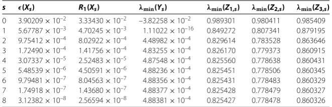
and R(X) = . × –, λmin(Y) = ., λmin(Z,) = .,

[image:13.595.132.463.624.731.2]

λmin(Z,) = .,λmin(Z,) = .. The other results are listed in Table .

Table 1 Error analysis for Example 4.1

s (Xs) R1(Xs) λmin(Ys) λmin(Z1,s) λmin(Z2,s) λmin(Z3,s)

0 3.90209×10–2 _3.33430_×₁₀–2 _–3.82258_×₁₀–2 _0.989301 _0.980411 _0.985409

1 5.67787×10–3 _4.70245_×₁₀–3 _1.11022_×₁₀–16 _0.849272 _0.807341 _0.879195

2 9.75412×10–4 _8.02922_×₁₀–4 _4.48982_×₁₀–4 _0.829614 _0.783528 _0.863646

3 1.72490×10–4 _1.41756_×₁₀–4 _4.83255_×₁₀–4 _0.826170 _0.779373 _0.860915

4 3.07337×10–5 _2.52483_×₁₀–5 _4.87548_×₁₀–4 _0.825560 _0.778638 _0.860431

5 5.48539×10–6 _4.50591_×₁₀–6 _4.88236_×₁₀–4 _0.825451 _0.778506 _0.860345

6 9.79481×10–7 _8.04563_×₁₀–7 _4.88356_×₁₀–4 _0.825431 _0.778483 _0.860329

7 1.74918×10–7 _1.43680_×₁₀–7 _4.88377_×₁₀–4 _0.825428 _0.778479 _0.860327

(14)

Example . Consider the matrix equation

X+A∗_X–A+A∗X–A+A∗X–A+A∗X–A=I, (.)

whereA,A,A, andAare given by

A=

⎛ ⎜ ⎜ ⎜ ⎝

. . . .

. . . .

. –. . .

. –. . .

⎞ ⎟ ⎟ ⎟ ⎠,

A=

⎛ ⎜ ⎜ ⎜ ⎝

. . . –.

. . . .

. . . –.

. . –. .

⎞ ⎟ ⎟ ⎟ ⎠,

A=

⎛ ⎜ ⎜ ⎜ ⎝

. . . .

. . . .

–. . –. .

–. –. . .

⎞ ⎟ ⎟ ⎟ ⎠,

A=

⎛ ⎜ ⎜ ⎜ ⎝

. . –. .

–. . . .

. . –. .

. –. . .

⎞ ⎟ ⎟ ⎟ ⎠.

We use Algorithm . to solve (.). After  iterations, we get the positive deﬁnite solution

X≈X=

⎛ ⎜ ⎜ ⎜ ⎝

. –. –. –.

–. . . –.

–. . . –.

–. –. –. .

⎞ ⎟ ⎟ ⎟ ⎠

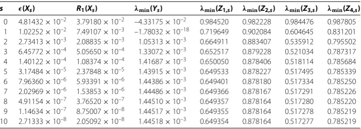
and R(X) = . × –, λmin(Y) = ., λmin(Z,) = .,

[image:14.595.118.478.603.732.2]

λmin(Z,) = .,λmin(Z,) = .,λmin(Z,) = .. The other results are listed in Table .

s (Xs) R1(Xs) λmin(Ys) λmin(Z1,s) λmin(Z2,s) λmin(Z3,s) λmin(Z4,s)

0 4.81432_×10–2 _3.79180_×₁₀–2 _–4.33175_×₁₀–2 _0.984520 _0.982228 _0.984476 _0.987805

1 1.02252_×10–2 _7.49107_×₁₀–3 _–1.78032_×₁₀–18 _0.719649 _0.902084 _0.604645 _0.831201

2 2.73413×10–3 _2.08835_×₁₀–3 _1.05313_×₁₀–3 _0.664911 _0.883407 _0.535912 _0.795502

3 6.45772×10–4 _5.05650_×₁₀–4 _1.33072_×₁₀–3 _0.652517 _0.879228 _0.521034 _0.787317

4 1.40122×10–4 _1.08374_×₁₀–4 _1.41687_×₁₀–3 _0.650050 _0.878406 _0.518114 _0.785684

5 3.17484×10–5 _2.37848_×₁₀–5 _1.43915_×₁₀–3 _0.649533 _0.878227 _0.517495 _0.785339

6 7.96360×10–6 _5.93391_×₁₀–6 _1.44386_×₁₀–3 _0.649401 _0.878180 _0.517334 _0.785250

7 2.02969×10–6 _1.53853_×₁₀–6 _1.44486_×₁₀–3 _0.649366 _0.878167 _0.517291 _0.785226

8 4.91154×10–7 _3.76520_×₁₀–7 _1.44510_×₁₀–3 _0.649357 _0.878164 _0.517280 _0.785220

9 1.14634×10–7 _8.75007_×₁₀–8 _1.44517_×₁₀–3 _0.649355 _0.878164 _0.517278 _0.785219

(15)

Example . Consider the matrix equation

X+A∗_X–A+A∗X–A=I, (.)

whereAandAare given as in Example . from []:

A=

⎛ ⎜ ⎝

. –. –.

. . –.

. –. .

⎞ ⎟ ⎠,

A=

⎛ ⎜ ⎝

. –. .

–. –. –.

. –. –.

⎞ ⎟ ⎠.

We use Algorithm . to solve (.). After  iterations, we get the positive deﬁnite solution

X≈X=

⎛ ⎜ ⎝

. –. –.

–. . –.

–. –. .

⎞ ⎟ ⎠

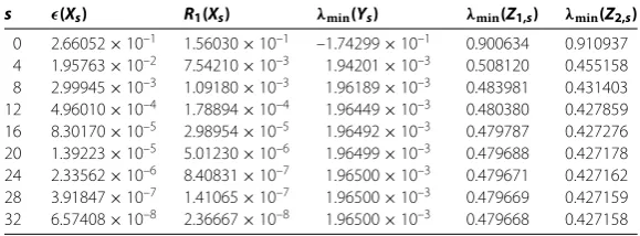
andR(X) = .×–,λmin(Y) = .,λmin(Z,) = .,λmin(Z,) = ..

The other results are listed in Table .

Example . Consider the matrix equation

X–A∗_X–A–A∗X–A–A∗X–A–A∗X–A=I, (.)

whereA,A,A, andAare given by

A=

⎛ ⎜ ⎝

. –. .

–. . .

. . .

⎞ ⎟

⎠, A=

⎛ ⎜ ⎝

. –. .

. . 

. –. .

⎞ ⎟ ⎠,

A=

⎛ ⎜ ⎝

–. . .

–. . .

. –. –.

⎞ ⎟

⎠, A=

⎛ ⎜ ⎝

 . .

. . .

. –. –.

⎞ ⎟ ⎠.

We use Algorithm . to solve (.). After  iterations, we get the positive deﬁnite solu-tion

X≈X=

⎛ ⎜ ⎝

. . –.

. . .

–. . .

⎞ ⎟ ⎠

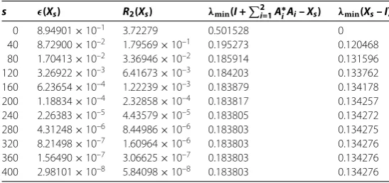
andR(X) = .×–, λmin(I+i=A∗iAi–X) = .,λmin(X–I) = ..

(16)

[image:16.595.152.442.98.205.2]

s (Xs) R1(Xs) λmin(Ys) λmin(Z1,s) λmin(Z2,s)

0 2.66052×10–1 _1.56030_×₁₀–1 _–1.74299_×₁₀–1 _0.900634 _0.910937

4 1.95763×10–2 _7.54210_×₁₀–3 _1.94201_×₁₀–3 _0.508120 _0.455158

8 2.99945×10–3 _1.09180_×₁₀–3 _1.96189_×₁₀–3 _0.483981 _0.431403

12 4.96010×10–4 _1.78894_×₁₀–4 _1.96449_×₁₀–3 _0.480380 _0.427859

[image:16.595.161.434.244.342.2]

16 8.30170×10–5 2.98954×10–5 1.96492×10–3 0.479787 0.427276 20 1.39223×10–5 5.01230×10–6 1.96499×10–3 0.479688 0.427178 24 2.33562×10–6 8.40831×10–7 1.96500×10–3 0.479671 0.427162 28 3.91847×10–7 1.41065×10–7 1.96500×10–3 0.479669 0.427159 32 6.57408_×10–8 _2.36667_×₁₀–8 _1.96500_×₁₀–3 _0.479668 _0.427158

s (Xs) R2(Xs) λmin(I +4i=1A∗iAi– Xs) λmin(Xs– I)

0 8.55046×10–1 _2.65 _0.715946 ₀

10 1.83959×10–1 _3.26477_×₁₀–1 _0.544118 _0.076489

20 1.06950×10–2 _1.87085_×₁₀–2 _0.493691 _0.098958

30 5.94976×10–4 _1.04066_×₁₀–3 _0.490594 _0.100375

40 3.30916×10–5 _5.78794_×₁₀–5 _0.490422 _0.100455

50 1.84048×10–6 _3.21913_×₁₀–6 _0.490412 _0.100459

60 1.02364×10–7 _1.79042_×₁₀–7 _0.490411 _0.100459

70 5.69327×10–9 _9.95792_×₁₀–9 _0.490411 _0.100459

Example . Consider the matrix equation

X–A∗_X–A–A∗X–A–A∗X–A=I, (.)

whereA,A, andAare given by

A=

⎛ ⎜ ⎜ ⎜ ⎝

.  –. .

.  . .

. . . .

. –. . .

⎞ ⎟ ⎟ ⎟

⎠, A=

⎛ ⎜ ⎜ ⎜ ⎝

 –. . .

. .  .

. –. . .

. .  .

⎞ ⎟ ⎟ ⎟ ⎠,

A=

⎛ ⎜ ⎜ ⎜ ⎝

–. . . .

–.  . –.

 –.  –.

. –. . .

⎞ ⎟ ⎟ ⎟ ⎠.

We use Algorithm . to solve (.). After  iterations, we get the positive deﬁnite solution

X≈X=

⎛ ⎜ ⎜ ⎜ ⎝

. . –. .

. . –. .

–. –. . .

. . . .

⎞ ⎟ ⎟ ⎟ ⎠

andR(X) = .×–,λmin(I+



i=A∗iAi–X) = .,λmin(X –I) = ..

(17)

[image:17.595.162.431.96.224.2]

0 2.10332×10–1 _2.95400_×₁₀–1 _0.047059 ₀

3 3.11244×10–2 _4.52684_×₁₀–2 _0.017503 _0.028153

6 5.17330×10–3 _8.36352_×₁₀–3 _0.023078 _0.023109

9 1.10730×10–3 _1.75717_×₁₀–3 _0.022155 _0.023907

12 2.28175×10–4 3.63481×10–4 0.022341 0.023751 15 4.73953×10–5 7.54424×10–5 0.022303 0.023783 18 9.83002×10–6 1.56497×10–5 0.022311 0.023776 21 2.03950×10–6 3.24685×10–6 0.022309 0.023778 24 4.23122_×10–7 _6.73607_×₁₀–7 _0.022310 _0.023777

27 8.77834_×10–8 _1.39750_×₁₀–7 _0.022310 _0.023777

[image:17.595.159.433.259.388.2]

30 1.82120×10–8 _2.89934_×₁₀–8 _0.022310 _0.023777

0 8.94901×10–1 _3.72279 _0.501528 ₀

40 8.72900×10–2 _1.79569_×₁₀–1 _0.195273 _0.120468

80 1.70413×10–2 _3.36946_×₁₀–2 _0.185914 _0.131596

120 3.26922×10–3 _6.41673_×₁₀–3 _0.184203 _0.133762

160 6.23654×10–4 _1.22239_×₁₀–3 _0.183879 _0.134178

200 1.18834×10–4 _2.32858_×₁₀–4 _0.183817 _0.134257

240 2.26383×10–5 _4.43579_×₁₀–5 _0.183805 _0.134272

280 4.31248×10–6 _8.44986_×₁₀–6 _0.183803 _0.134275

320 8.21498×10–7 1.60964×10–6 0.183803 0.134276 360 1.56490×10–7 3.06625×10–7 0.183803 0.134276 400 2.98101×10–8 5.84098×10–8 0.183803 0.134276

Example . Consider the matrix equation

X–A∗_X–A–A∗X–A=I, (.)

whereAandAare given as in Example . from []:

A=

⎛ ⎜ ⎝

. . .

. . .

. . .

⎞ ⎟ ⎠,

A=

⎛ ⎜ ⎝

. . .

. . .

. . .

⎞ ⎟ ⎠.

We use Algorithm . to solve (.). After  iterations, we get the positive deﬁnite so-lution

X≈X=

⎛ ⎜ ⎝

. . .

. . .

. . .

⎞ ⎟ ⎠

andR(X) = .×–,λmin(I+i=A∗iAi–X) = .,λmin(X–I) = ..

(18)

5 Conclusion

In this paper, we investigate the nonlinear matrix equationsX±m_i_=A∗_iX–ni_A

i=I, where

ni,i= , , . . . ,m, are positive integers. Necessary and suﬃcient conditions for the existence

of positive definite solutions are derived. Iterative algorithms are proposed to compute the positive definite solutions of these equations. Moreover, some numerical examples are given to illustrate the effectiveness and rapidly convergence rate (small run time) of the proposed iterative algorithms (see values of(Xs),R(Xs), andR(Xs)). Also, the values

ofλminshow that the solutions of the matrix equations satisfy the necessary conditions.

Competing interests

The author declares to have no competing interests.

Acknowledgements

The author is grateful to the editor and the reviewer for important comments and suggestions, which improved the quality of the paper.

Received: 15 February 2015 Accepted: 15 April 2015

References

1. Anderson, WN, Morley, TD, Trapp, GE: Positive solutions toX=A–BX–1_B∗_{. Linear Algebra Appl.}₁₃₄_{, 53-62 (1990)}

2. Engwerda, JC: On the existence of a positive deﬁnite solution of the matrix equationX+AT_X–1_A₌_I_{. Linear Algebra}

Appl.194, 91-108 (1993)

3. Ferrante, A, Levy, BC: Hermitian solutions of the equationX=Q+NX–1_N∗_{. Linear Algebra Appl.}₂₄₇_{, 359-373 (1996)}

4. Zhan, X: Computing the extremal positive deﬁnite solutions of a matrix equation. SIAM J. Sci. Comput.17, 1167-1174 (1996)

5. He, YM, Long, JH: On the Hermitian positive deﬁnite solution of the nonlinear matrix equationX+m_i₌₁A∗_iX–1_A

i=I. Appl. Math. Comput.216, 3480-3485 (2010)

6. Duan, X, Wang, Q, Liao, A: On the matrix equationX–m_i₌₁N∗_iX–1_N

i=Iarising in an interpolation problem. Linear Multilinear Algebra61, 1192-1205 (2013)

7. Sakhnovich, LA: Interpolation Theory and Its Applications. Mathematics and Its Applications. Kluwer Academic, Dordrecht (1997)

8. Cheng, M, Xu, S: Perturbation analysis of the Hermitian positive deﬁnite solution of the matrix equation

X–A∗X–2_A₌_I_{. Linear Algebra Appl.}₃₉₄_{, 39-51 (2005)}

9. Duan, X, Li, C, Liao, A: Solutions and perturbation analysis for the nonlinear matrix equationX+mi=1A∗iX–1Ai=I. Appl. Math. Comput.218, 4458-4466 (2011)

10. El-Sayed, SM, Al-Dubiban, AM: On positive deﬁnite solutions of the nonlinear matrix equationX+A∗X–n_A₌_I_{. Appl.} Math. Comput.151, 533-541 (2004)

11. Hasanov, VI: Notes on two perturbation estimates of the extreme solutions to the equationsX_±A∗X–1_A₌_Q_{. Appl.}

Math. Comput.216, 1355-1362 (2010)

12. Ivanov, IG: On positive deﬁnite solutions of the family of matrix equationsX+A∗X–n_A₌_Q_{. J. Comput. Appl. Math.}

193, 277-301 (2006)

13. Lin, WW, Xu, SF: Convergence analysis of structure-preserving doubling algorithms for Riccati-type matrix equations. SIAM J. Matrix Anal. Appl.28, 26-39 (2006)

14. Chiang, CY, Chu, EKW, Guo, CH, Huang, TM, Lin, WW, Xu, SF: Convergence analysis of the doubling algorithm for several nonlinear matrix equations in the critical case. SIAM J. Matrix Anal. Appl.31, 227-247 (2009)

15. Ivanov, IG, Hasanov, VI, Minchev, BV: On matrix equationsX±A∗X–2_A₌_I_{. Linear Algebra Appl.}₃₂₆_{, 27-44 (2001)}

16. El-Sayed, SM: Two iteration processes for computing positive deﬁnite solutions of the equationX–A∗X–n_A₌_Q_. Comput. Math. Appl.41, 579-588 (2001)

17. El-Sayed, SM, Ran, ACM: On an iterative method for solving a class of nonlinear matrix equations. SIAM J. Matrix Anal. Appl.23, 632-645 (2001)

18. Hasanov, VI, Ivanov, IG: Solutions and perturbation estimates for the matrix equationsX±A∗X–n_A₌_Q_{. Appl. Math.} Comput.156, 513-525 (2004)

19. Hasanov, VI: Positive deﬁnite solutions of the matrix equationsX±A∗X–q_A₌_Q_{. Linear Algebra Appl.}₄₀₄_{, 166-182} (2005)

20. Duan, XF, Wang, QW, Li, CM: Perturbation analysis for the positive deﬁnite solution of the nonlinear matrix equation

X–mi=1A∗iXδiAi=Q. J. Appl. Math. Inform.30, 655-663 (2012)

21. Liu, XG, Gao, H: On the positive deﬁnite solutions of the matrix equationsXs_±_AT_X–t_A₌_I_{n. Linear Algebra Appl.}₃₆₈_, 83-97 (2003)

22. Long, JH, Hu, XY, Zhang, L: Improved Newton’s method with exact linear searches to solve quadratic matrix equation. J. Comput. Appl. Math.222, 645-654 (2008)

23. Yao, G, Liao, A, Duan, X: Positive deﬁnite solution of the matrix equationX=Q+AH₍_I_⊗_X_–_C₎–δ_A∗_{. Electron. J. Linear}

Algebra21, 76-84 (2010)

24. Ivanov, IG, El-Sayed, SM: Properties of positive deﬁnite solutions of the equationX+A∗X–2_A₌_I_{. Linear Algebra Appl.} 279, 303-316 (1998)