Probabilistic 2D Point Interpolation and Extrapolation via Data
Modeling
Dariusz Jacek Jakóbczak
Department of Electronics and Computer Science, Technical University of Koszalin, Sniadeckich 2, 75-453 Koszalin, Poland
E-mail: [email protected]
Keywords: 2D data interpolation, Hurwitz-Radon matrices, MHR method, probabilistic modeling, curve extrapolation
Received: June 25, 2014
Mathematics and computer science are interested in methods of 2D curve interpolation and extrapolation using the set of key points (knots). A proposed method of Hurwitz- Radon Matrices (MHR) is such a method. This novel method is based on the family of Hurwitz-Radon (HR) matrices which possess columns composed of orthogonal vectors. Two-dimensional curve is interpolated via different functions as probability distribution functions: polynomial, sinus, cosine, tangent, cotangent, logarithm, exponent, arcsin, arccos, arctan, arcctg or power function, also inverse functions. It is shown how to build the orthogonal matrix operator and how to use it in a process of curve reconstruction.
Povzetek: Opisana je nova metoda 2D interpolacije in ekstrapolacije krivulj.
1
Introduction
Curve interpolation and extrapolation [1] represents one of the most important problems in mathematics: how to model the curve [2] via discrete set of two-dimensional points [3]? Also the matter of curve representation and parameterization is still opened in mathematics and computer sciences [4]. The author wants to approach a problem of curve modeling by characteristic points. Proposed method relies on functional modeling of curve points situated between the basic set of the nodes or outside the nodes. The functions that are used in calculations represent whole family of elementary functions with inverse functions: polynomials, trigonometric, cyclometric, logarithmic, exponential and power function. These functions are treated as probability distribution functions in the range [0,1]. Nowadays methods apply mainly polynomial functions, for example Bernstein polynomials in Bezier curves, splines and NURBS [5]. Numerical methods for data interpolation or extrapolation are based on polynomial or trigonometric functions, for example Lagrange, Newton, Aitken and Hermite methods. These methods have some weak sides [6] and are not sufficient for curve interpolation and extrapolation in the situations when the curve cannot be build by polynomials or trigonometric functions. Proposed 2D curve interpolation and extrapolation is the functional modeling via any elementary functions and it helps us to fit the curve during the computations.
The main contributions of the paper are dealing with presentation the method that connects such problems as: interpolation, extrapolation, modeling, numerical methods and probabilistic methods. This is new approach to these problems. Differences from the previous papers of the author are connected with calculations without
matrices (N = 1), new probabilistic distribution functions and novel look on shape modeling and curve reconstruction.
The method of Hurwitz-Radon Matrices (MHR) requires minimal assumptions: the only information about a curve is the set of at least two nodes. Proposed method of Hurwitz-Radon Matrices (MHR) is applied in curve modeling via different coefficients: polynomial, sinusoidal, cosinusoidal, tangent, cotangent, logarithmic, exponential, arcsin, arccos, arctan, arcctg or power. Function for MHR calculations is chosen individually at each interpolation and it represents probability
distribution function of parameter α [0,1] for every
point situated between two interpolation knots. MHR method uses two-dimensional vectors (x,y) for curve modeling - knots (xi,yi)R2in MHR method:
1. MHR version with no matrices (N = 1) needs 2 knots or more;
2. At least five knots (x1,y1), (x2,y2), (x3,y3), (x4,y4) and (x5,y5) if MHR method is implemented with matrices of dimension N = 2;
3. For more precise modeling knots ought to be settled at key points of the curve, for example local minimum or maximum and at least one node between two successive local extrema.
Condition 2 is connected with important features of MHR method: MHR version with matrices of dimension
N = 2 (MHR-2) requires at least five nodes, MHR
question: how to interpolate end extrapolate the curve by a set of knots?
Figure 1: Knots of the curve before modelling.
Coefficients for curve modeling are computed using probability distribution functions: polynomials, power functions, sinus, cosine, tangent, cotangent, logarithm, exponent or arcsin, arccos, arctan, arcctg.
2
Probabilistic 2D interpolation and
extrapolation
The method of Hurwitz – Radon Matrices (MHR) is computing points between two successive nodes of the curve: calculated points are interpolated and parameterized for real number [0,1] in the range of two successive nodes. Data extrapolation is possible for
< 0 or> 1. MHR calculations are dealing with square matrices of dimension N = 1, 2, 4 or 8. Matrices Ai,
i=1,2…m satisfying
AjAk+ AkAj= 0, Aj2= -I for j≠ k; j, k = 1,2...m
are called a family of Hurwitz - Radon matrices. They were discussed by Adolf Hurwitz and Johann Radon separately in 1923. A family of Hurwitz-Radon (HR) matrices [7] are skew-symmetric: Ai
T
= -Aiand Ai
-1 = - Ai.
Only for dimensions N = 1, 2, 4 or 8 the family of HR matrices consists of N - 1 matrices. For N = 1 there is no matrices but only calculations with real numbers. For
N=2: . 0 1 1 0 1 A
For N = 4 there are three HR matrices with integer entries: , 0 1 0 0 1 0 0 0 0 0 0 1 0 0 1 0 1 A , 0 0 1 0 0 0 0 1 1 0 0 0 0 1 0 0 2 A . 0 0 0 1 0 0 1 0 0 1 0 0 1 0 0 0 3 A
For N = 8 we have seven HR matrices with elements 0, ±1. So far HR matrices have found applications in Space-Time Block Coding (STBC) [8] and orthogonal design [9], in signal processing [10] and Hamiltonian Neural Nets [11].
How coordinates of knots are applied for interpolation and extrapolation? If knots are represented by the following points {(xi,yi), i = 1,2, …,n} then HR
matrices combined with the identity matrix INare used to
build the orthogonal Hurwitz - Radon Operator (OHR).
For point p1=(x1,y1) and x1≠0OHR of dimension N = 1 is the matrix (real number) M1:
. 1 ) ( 1 1 1 1 2 1 1 1 x y y x x pM (0)
For points p1=(x1,y1) and p2=(x2,y2) OHR of dimension
N=2 is build via matrix M2:
2 2 1 1 1 2 2 1 2 1 1 2 2 2 1 1 2 2 2 1 2 1 2 1 ) , ( y x y x y x y x y x y x y x y x x x p p
M . (1)
For points p1=(x1,y1), p2=(x2,y2), p3=(x3,y3) and p4=(x4,y4) OHR M4 of dimension N = 4 is introduced:
0 1 2 3 1 0 3 2 2 3 0 1 3 2 1 0 2 4 2 3 2 2 2 1 4 3 2 1 4 1 ) , , , ( u u u u u u u u u u u u u u u u x x x x p p p p M (2) where 4 4 3 3 2 2 1 1
0 xy x y x y x y
u ,
3 4 4 3 1 2 2 1
1 xy x y x y x y
u ,
2 4 1 3 4 2 3 1
2 xy x y x y x y
u ,
1 4 2 3 3 2 4 1
3 x y x y x y x y
u .
For knots p1=(x1,y1), p2=(x2,y2),… andp8=(x8,y8) OHR M8 of dimension N = 8 is constructed [12] similarly as (1) and (2):
0 1 2 3 4 5 6 7 1 0 3 2 5 4 7 6 2 3 0 1 6 7 4 5 3 2 1 0 7 6 5 4 4 5 6 7 0 1 2 3 5 4 7 6 1 0 3 2 6 7 4 5 2 3 0 1 7 6 5 4 3 2 1 0 8 1 2 8 2 1 8 1 ) ... , ( u u u u u u u u u u u u u u u u u u u u u u u u u u u u u u u u u u u u u u u u u u u u u u u u u u u u u u u u u u u u u u u u x p p p M i i (3) where 8 7 6 5 4 3 2 1 1 2 3 4 5 6 7 8 2 1 4 3 6 5 8 7 3 4 1 2 7 8 5 6 4 3 2 1 8 7 6 5 5 6 7 8 1 2 3 4 6 5 8 7 2 1 4 3 7 8 5 6 3 4 1 2 8 7 6 5 4 3 2 1 x x x x x x x x y y y y y y y y y y y y y y y y y y y y y y y y y y y y y y y y y y y y y y y y y y y y y y y y y y y y y y y y y y y y y y y y u (4)and u = (u0, u1,…, u7) T
(4). OHR operators MN (0)-(3)
satisfy the condition of interpolation
MNx = y (5)
for x = (x1,x2…,xN)
T
RN, x0, y = (y1,y2…,yN)
T
RN
and N = 1, 2, 4 or 8.
2.1
Distribution functions in MHR
interpolation and extrapolation
c = a + +(1 -)b for
a b
c b
[0,1]. (6)
The weighted average OHR operator M of dimension N = 1, 2, 4 or 8 is build:
B A
M (1) . (7)
The OHR matrix A is constructed (1)-(3) by every second knot p1=(x1=a,y1), p3=(x3,y3), …andp2N-1=(x2N-1,y2N-1):
A = MN(p1, p3,...,p2N-1).
The OHR matrix B is computed (1)-(3) by knots
p2=(x2=b,y2), p4=(x4,y4),… andp2N=(x2N,y2N):
B = MN(p2, p4,...,p2N).
Vector of first coordinates C is defined for
ci=x2i-1+ (1-)x2i , i= 1, 2,…,N (8) and C = [c1, c2,…,cN]T. The formula to calculate second
coordinates y(ci) is similar to the interpolation formula
(5):
C M C
Y( ) (9)
where Y(C) = [y(c1), y(c2),…, y(cN)]T. So interpolated
value y(ci) from (9) depends on two, four, eight or
sixteen (2N) successive nodes. For example N=1 results in computations without matrices:
1 1 1 1( )
x y p M
A ,
2 2 2 1( )
x y p M
B ,
C = c1=x1+ (1-)x2,
1 2 2
1 1
1) ( (1 ) )
( )
( c
x y x
y c y C
Y ,
1 2 2 2
1 1 2
1
1) (1 )(1 ) (1 ) (1 )
( x
x y x
x y y
y c
y
. (10)
Formula (10) shows a clear calculation for interpolation of any point between two successive nodes (x1,y1) and
(x2,y2). Key question is dealing with coefficient γin (7).
Basic MHR version meansγ= α and then (10):
). )(
1 ( ) 1 ( )
( 1
2 2 2 1 1 2
2 1
2
1 x
x y x x y y
y c
y
(11)
Formula (11) represents the simplest way of MHR calculations (N = 1, γ = α) and it differs from linear
interpolation y(c)y1(1)y2. MHR is not a linear interpolation.
Each interpolation requires specific distribution of
parameter α (7) and γ depends on parameter α[0,1]:
γ = F(α), F:[0,1]→[0,1], F(0) = 0, F(1) = 1
and F is strictly monotonic.
Coefficient γ is calculated using different functions (polynomials, power functions, sinus, cosine, tangent, cotangent, logarithm, exponent, arcsin, arccos, arctan or arcctg, also inverse functions) and choice of function is connected with initial requirements and curve
specifications. Different values of coefficient γ are
connected with applied functions F(α). These functions
(12)-(41) represent the probability distribution functions for randomvariable α[0,1] and real number s > 0:
1. power function
γ = αs with s > 0. (12)
For s= 1: basic version of MHR method when γ = α.
2. sinus
γ =sin(αs· π/2) , s > 0 (13)
or
γ =sins(α · π/2) , s > 0. (14)
For s= 1: γ =sin(α · π/2). (15)
3. cosine
γ = 1-cos(αs· π/2) , s > 0 (16)
or
γ = 1-coss(α · π/2) , s > 0. (17)
For s= 1: γ = 1-cos(α · π/2). (18)
4. tangent
γ =tan(αs· π/4) , s > 0 (19)
or
γ =tans(α · π/4) , s > 0. (20)
For s= 1: γ =tan(α · π/4). (21)
5. logarithm
γ =log2(αs+ 1) , s > 0 (22) or
γ =log2
s
(α + 1) , s > 0. (23)
For s= 1: γ =log2(α + 1). (24) 6. exponent
s a a
) 1
1 (
, s > 0 and a > 0 and a≠ 1. (25)
For s = 1 and a= 2: γ = 2α–1. (26)
7. arc sine
γ = 2/π·arcsin(αs) , s > 0 (27)
or
γ = (2/π·arcsinα)s, s > 0. (28)
For s= 1: γ = 2/π·arcsin(α). (29) 8. arc cosine
γ = 1-2/π·arccos(αs) , s > 0 (30) or
γ = 1-(2/π·arccosα)s, s > 0. (31)
For s= 1: γ = 1-2/π·arccos(α). (32) 9. arc tangent
γ = 4/π·arctan(αs) , s > 0 (33)
or
γ = (4/π·arctanα)s, s > 0. (34)
For s= 1: γ = 4/π·arctan(α). (35) 10. cotangent
γ =ctg(π/2 – αs· π/4) , s > 0 (36)
or
γ =ctgs(π/2-α · π/4), s > 0. (37)
11. arc cotangent
γ = 2-4/π· arcctg(αs) , s > 0 (39)
or
γ = (2-4/π·arcctgα)s, s > 0. (40)
For s= 1: γ = 2-4/π·arcctg(α). (41)
Functions used in γ calculations (12)-(41) are strictly
monotonic for random variable α [0,1] as γ = F(α) is
probability distribution function. Also inverse function
F-1(α) is appropriate for γ calculations. Choice of
function and value s depends on curve specifications and individual requirements. Interpolating of coordinates for curve points using (6)-(9) is called by author the method of Hurwitz - Radon Matrices (MHR) [15]. So here are five steps of MHR interpolation:
Step 1: Choice of knots at key points.
Step 2: Fixing the dimension of matrices N = 1, 2, 4 or 8: N = 1 is the most universal for calculations (it needs only
two nodes to compute unknown points between them) and it has the lowest computational costs (10); MHR with N = 2 uses four successive nodes to compute unknown coordinate; MHR version for N = 4 applies eight successive nodes to get unknown point and MHR with N = 8 needs sixteen successive nodes to calculate unknown coordinate (it has the biggest computational costs).
Step 3: Choice of distribution γ = F(α): basic distribution for γ = α.
Step 4: Determining values of α: α = 0.1, 0.2…0.9 (nine points) or 0.01, 0.02…0.99 (99 points) or others.
Step 5: The computations (9).
These five steps can be treated as the algorithm of MHR method of curve modeling and interpolation (6)-(9).
Considering nowadays used probability distribution
functions for random variable α[0,1] - one distribution
is dealing with the range [0,1]: beta distribution. Probability density function f for random variable α
[0,1] is:
r s
c
f() (1) , s≥ 0,r≥0 (42)
When r = 0 probability density function (42) represents
s c
f() and then probability distribution function F is like (12), for example f()32 and γ=α3. If s and r
are positive integer numbers then γ is the polynomial, for
example f()6(1) and γ = 3α2-2α3. So beta
distribution gives us coefficient γ in (7) as polynomial
because of interdependence between probability density f and distribution F functions:
) ( ' ) ( F
f , F( ) f(t)dt
0
. (43)
For example (43): f()e and 1
) 1 ( )
(
F e .
What is very important: two curves may have the same set of nodes but different Nor γ results in different
interpolations (Fig.6-13). Here are some applications of
MHR method with basic version (γ = α): MHR-2 is
MHR version with matrices of dimension N = 2 and MHR-4 means MHR version with matrices of dimension
N = 4.
Figure 2: Function f(x) = x3+x2-x+1 with 396 interpolated points using basic MHR-2 with 5 nodes.
Figure 3: Function f(x) = x3+ln(7-x) with 396 interpolated points using basic MHR-2 with 5 nodes.
Figure 4: Function f(x) = x3+2x-1 with 792 interpolated points using basic MHR-4 with 9 nodes.
Figure 5: Function f(x) = 3-2xwith 396 interpolated points using basic MHR-2 with 5 nodes.
Figures 2-5 show interpolation of continues functions connected with determined formula. So these functions are interpolated and modeled. Without knowledge about the formula, curve interpolation has to
implement the coefficients γ (12)-(43), but MHR is not
limited only to these coefficients. Each strictly monotonic function F between points (0;0) and (1;1) can be used in MHR interpolation. MHR 2D data extrapolation is possible for< 0 or>1.
3
Implementations of 2D
probabilistic interpolation
Curve knots (0.1;10), (0.2;5), (0.4;2.5), (1;1) and (2;5) from Fig.1 are used in some examples of MHR
interpolation with different γ. Points of the curve are
matrices of dimension N = 2 in examples 2 -8 for α = 0.1, 0.2,…,0.9.
Example 1
Curve interpolation for N= 1 and γ = α.
Figure 6: Modeling without matrices (N = 1) for nine reconstructed points between nodes.
Example 2
Sinusoidal interpolation with γ =sin(α · π/2).
Figure 7: Sinusoidal modeling with nine reconstructed curve points between nodes.
Example 3
Tangent interpolation for γ =tan(α · π/4).
Figure 8: Tangent curve modeling with nine interpolated points between nodes.
Example 4
Tangent interpolation with γ =tan(αs· π/4) ands = 1.5.
Figure 9: Tangent modeling with nine recovered points between nodes.
Example 5
Tangent curve interpolation for γ =tan(αs· π/4) ands =
1.797.
Figure 10: Tangent modeling with nine reconstructed points between nodes.
Example 6
Sinusoidal interpolation with γ = sin(αs · π/2) and s =
2.759.
Figure 11: Sinusoidal modeling with nine interpolated curve points between nodes.
Example 7
Power function modeling for γ = αsand s = 2.1205.
Figure 12: Power function curve modeling with nine recovered points between nodes.
Example 8
Logarithmic curve modeling with γ =log2(α
s
+ 1) and s = 2.533.
Figure 13: Logarithmic modeling with nine reconstructed points between nodes.
parameter γ. This parameter is treated as probability
distribution function for each curve.
4
MHR 2D modeling versus
polynomial interpolation
4.1
Example 4.1
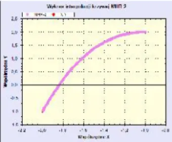
Let us consider a graph of function f(x) = 2/x in range [0.4,1.6]. There are given five interpolation nodes for x = 0.4, 0.7, 1.0, 1.3, 1.6. The curve y = 2/x reconstructed by basic MHR method (12) with N = 2 for s = 1 looks not precisely:
Figure 14: The curve y = 2/x reconstructed by MHR method forγ = α(7) and five nodes together with 36 computed points.
Lagrange interpolation polynomial is not to be accepted:
Figure 15: Polynomial interpolation of function y = 1/x is out of acceptation.
For better reconstruction of the curve, appropriate parameter s in MHR method (12) is calculated. Choice of parameter s is connected with comparison of accurate values wi for function f(x) = 2/x in control points pi,
situated in the middle between interpolation nodes (=0.5), and values in control points pi computed by
MHR method. Control points are settled in the middle between interpolation nodes, because interpolation error of MHR method is the biggest. Choice of coefficient s is done by criterion: difference between precise values wi
and values reconstructed by MHR method is the smallest. Control points piin this example are established for xi=
0.55, 0.85, 1.15, 1.45. Four values of the curve are compared for parameter s = 0.1, 0.2, 0.3, 0.4, 0.5, 0.6,
0.7, 0.8, 0.9, 1.0, 1.1, 1.2, 1.3, 1.4, 1.5, 1.6, 1.7, 1.8, 1.9, 2.0. The smallest difference is calculated for s = 1.5:
(44)
Calculations for average OHR operator M (7) are done:
, ;
, .
Computed values appear in (44). Other results: a) s=0.1
b) s=0.2:
c) s=0.3:
d) s=0.4:
e) s=0.5:
f) s=0.6:
g) s=0.7:
h) s=0.8:
i) s=0.9:
j) s=1:
k) s=1.1:
l) s=1.2:
m) s=1.3:
n) s=1.4:
o) s=1.6:
p) s=1.7:
q) s=1.8:
r) s=1.9:
s) s=2.0:
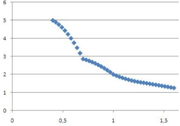
Figure 16: The curve y = 2/x modeled via MHR method (12) for s = 1.5 and five nodes together with 36 reconstructed points.
Figure 16 represents the curve y = 2/x more precisely then classical interpolation and Figure 14. If we would like to have better parameter s (with two digits after coma), calculations are done:
a) s=1.49:
b) s=1.51:
c) s=1.52:
d) s=1.53:
e) s=1.54:
f) s=1.55:
g) s=1.56:
h) s=1.57:
i) s=1.58:
j) s=1.59:
Model of the curve for s = 1.56 in (12) is more accurate then with s = 1.5.
Convexity of reconstructed curve is very important factor in MHR method with parameter s. Appropriate choice of parameter s is connected with regulation and controlling of convexity: model of the curve (Fig. 16) preserves monotonicity and convexity.
4.2
Example 4.2
This example considers a graph of function
) 5 1 /( 1 )
( 2
x x
f in the range [-1,1]:
Figure 17: A graph of function ( ) 1/(1 5 2) x x
f in range [-1,1].
There are given five interpolation nodes for x = -1.0, -0.5, 0, 0.5, 1.0. It is an example of function with useless Lagrange interpolation polynomial: Runge phenomenon and unpleasant two minima.
Figure 18: Lagrange interpolation polynomial differs extremely from a graph of function ( ) 1/(1 5 2)
x x
f .
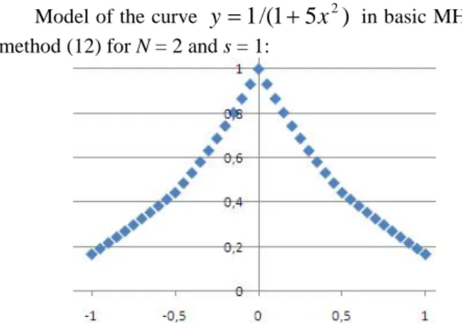
Model of the curve
y
1
/(
1
5
x
2)
in basic MHR method (12) for N = 2 and s = 1:Figure 19: The curve 1/(1 5 2)
x
y modeled via MHR method for γ = α (7) and five nodes together with 36 reconstructed points.
Reconstructed curve (Fig. 19) preserves monotonicity and symmetry for s = 1. Comparing precise values wi with values computed by MHR method in
control points pi, fixed for xi = -0.75, -0.25, 0.25, 0.75,
identical the best results appear for s = 1 (12):
(45)
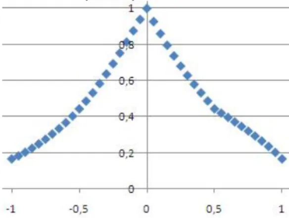
symmetric- look at values in (45). So if a case s = 1 appears among the best results, then model ought to be built for s = 1. And if a case s = 1 does not appear among the best results, then model ought to be built for s near by 1. Here is an example of reconstructed curve for s=1.5 (without feature of symmetry):
Figure 20: The curve 1/(1 5 2)
x
y modeled via MHR method for s = 1.5 (12) and five nodes together with 36 reconstructed points.
The best model of the curve y1/(15x2), built by MHR method for s = 1 (Fig. 19), preserves monotonicity and symmetry. Convexity of the function (Fig. 17) can make some troubles.
5
Future research directions
Future works with MHR method are connected with object recognition after geometrical transformations of curve (translations, rotations, scaling)- only nodes are transformed and new curve (for example contour of the object) for new nodes is reconstructed. Also estimation of object area in the plane, using nodes of object contour, will be possible by MHR interpolation. Object area is significant feature for object recognition. Future works are dealing with smoothing the curve, parameterization of whole curve and possibility to apply MHR method to three-dimensional curves. Also case of equidistance nodes must be studied with all details. Another future research direction is to apply MHR method in artificial intelligence and computer vision, for example
identification of a specific person’s face or fingerprint,
optical character recognition (OCR), image restoration, content-based image retrieval and pose estimation. Future works are connected with object recognition for any set of contour points. There are several specialized tasks based on recognition to consider and it is important to use the shape of whole contour for identification and detection of persons, vehicles or other objects. Other applications of MHR method will be directed to computer graphics, modeling and image processing.
6
Conclusion
The method of Hurwitz-Radon Matrices (MHR) enables interpolation of two-dimensional curves using different coefficients γ: polynomial, sinusoidal, cosinusoidal,
tangent, cotangent, logarithmic, exponential, arcsin,
arccos, arctan, arcctg or power function [16], also inverse
functions. Function for γ calculations is chosen
individually at each curve modeling and it is treated as
probability distribution function: γ depends on initial
requirements and curve specifications. MHR method leads to curve interpolation via discrete set of fixed knots. So MHR makes possible the combination of two important problems: interpolation and modeling. Main features of MHR method are:
a) the smaller distance between knots the better; b) calculations for coordinate x close to zero and
near by extremum require more attention; c) MHR interpolation of the function is more
precise then linear interpolation;
d) minimum two interpolation knots for calculations without matrices when N=1, but MHR is not a linear interpolation;
e) interpolation of L points is connected with the computational cost of rank O(L);
f) MHR is well-conditioned method (orthogonal matrices)[17];
g) coefficient γ is crucial in the process of curve
probabilistic interpolation and it is computed individually for a single curve;
h) MHR 2D data extrapolation is possible for< 0 or> 1.
Future works are going to: choice and features of
coefficient γ, implementation of MHR in object
recognition [18], shape geometry, contour modeling and parameterization [19].
References
[1] Collins II, G.W.: Fundamental Numerical Methods and Data Analysis. Case Western Reserve University (2003)
[2] Chapra, S.C.: Applied Numerical Methods. McGraw-Hill (2012)
[3] Ralston, A., Rabinowitz, P.: A First Course in Numerical Analysis – Second Edition. Dover Publications, New York (2001)
[4] Zhang, D., Lu, G.: Review of Shape Representation and Description Techniques. Pattern Recognition 1(37), 1-19 (2004)
[5] Schumaker, L.L.: Spline Functions: Basic Theory. Cambridge Mathematical Library (2007)
[6] Dahlquist, G., Bjoerck, A.: Numerical Methods. Prentice Hall, New York (1974)
[7] Eckmann, B.: Topology, Algebra, Analysis-Relations and Missing Links. Notices of the American Mathematical Society 5(46), 520-527 (1999)
[8] Citko, W., Jakóbczak, D., Sieńko, W.:On Hurwitz
-Radon Matrices Based Signal Processing. Workshop Signal Processing at Poznan University of Technology (2005)
[10] Sieńko, W., Citko, W., Wilamowski, B.:
Hamiltonian Neural Nets as a Universal Signal Processor. 28th Annual Conference of the IEEE Industrial Electronics Society IECON (2002)
[11] Sieńko, W., Citko, W.: Hamiltonian Neural Net
Based Signal Processing. The International Conference on Signal and Electronic System ICSES (2002)
[12] Jakóbczak, D.: 2D and 3D Image Modeling Using Hurwitz-Radon Matrices. Polish Journal of Environmental Studies 4A(16), 104-107 (2007) [13] Jakóbczak, D.: Shape Representation and Shape
Coefficients via Method of Hurwitz-Radon Matrices. Lecture Notes in Computer Science 6374 (Computer Vision and Graphics: Proc. ICCVG 2010, Part I), Springer-Verlag Berlin Heidelberg, 411-419 (2010)
[14] Jakóbczak, D.: Curve Interpolation Using Hurwitz-Radon Matrices. Polish Journal of Environmental Studies 3B(18), 126-130 (2009)
[15] Jakóbczak, D.: Application of Hurwitz-Radon Matrices in Shape Representation. In: Banaszak, Z.,
Świć, A. (eds.) Applied Computer Science:
Modelling of Production Processes 1(6), pp. 63-74.
Lublin University of Technology Press, Lublin (2010)
[16] Jakóbczak, D.: Object Modeling Using Method of Hurwitz-Radon Matrices of Rank k. In: Wolski, W., Borawski, M. (eds.) Computer Graphics: Selected Issues, pp. 79-90. University of Szczecin Press, Szczecin (2010)
[17] Jakóbczak, D.: Implementation of Hurwitz-Radon
Matrices in Shape Representation. In: Choraś, R.S.
(ed.) Advances in Intelligent and Soft Computing 84, Image Processing and Communications: Challenges 2, pp. 39-50. Springer-Verlag, Berlin Heidelberg (2010)
[18] Jakóbczak, D.: Object Recognition via Contour Points Reconstruction Using Hurwitz-Radon Matrices. In: Józefczyk, J., Orski, D. (eds.) Knowledge-Based Intelligent System Advancements: Systemic and Cybernetic Approaches, pp. 87-107. IGI Global, Hershey PA, USA (2011)