A Contribution to Triangulation
Algorithms for Simple Polygons
Marko Lamot
1, Borut
Zalik
ˇ
21Hermes Softlab, Ljubljana, Slovenia
2BorutZalik, University of Maribor, Faculty of Electrical Engineering and Computer Sciences, Maribor, Sloveniaˇ
Decomposing simple polygon into simpler components is one of the basic tasks in computational geometry and its applications. The most important simple polygon de-composition is triangulation. The known algorithms for polygon triangulation can be classified into three groups: algorithms based on diagonal inserting, algorithms based on Delaunay triangulation, and the algorithms using Steiner points. The paper briefly explains the most popular algorithms from each group and summarizes the common features of the groups. After that four algorithms based on diagonals insertion are tested: a recursive diagonal inserting algorithm, an ear cutting algorithm, Kong’s Graham scan algorithm, and Seidel’s randomized incremental algorithm. An analysis con-cerning speed, the quality of the output triangles and the ability to handle holes is done at the end.
Keywords: simple polygons, simple polygon triangula-tion, Steiner points, constrained Delaunay triangulation
1. Introduction
Polygons are very convenient for computer rep-resentation of the boundary of the objects from the real world. Because polygons can be very complex(they can include a few thousand ver-tices, they may be concave and may include nested holes), often there is the need to decom-pose the polygons into simpler components that can be easily and rapidly handled. There are many ideas how to perform this decomposition. Planar polygons can be, for example, decom-posed into triangles, trapezoids or even star-shaped polygons. Computing the triangulation of a polygon is a fundamental algorithm in the computational geometry. It is also the most investigated partitioning method. In computer graphics, polygon triangulation algorithms are
widely used for tessellating curved geometries, such as those described by spline.
The paper gives a brief summary of existing triangulation techniques and a comparison be-tween them. It is organized into eight sections. The second chapter introduces the fundamen-tal terminology, and in the third chapter diag-onal inserting algorithms are dealt with. The fourth section explains the constrained Delau-nay triangulation. The fifth section describes triangulation techniques that use Steiner points. The sixth section summarizes the common fea-tures of all three groups of polygon triangula-tion algorithms. The seventh sectriangula-tion contains the comparison of triangulation methods based on the diagonal insertion. An analysis concern-ing speed, the quality of the output triangles, and the ability to handle holes is done. The last section summarizes the work.
2. Background
Every simple polygonP(a polygon is simple if its edges cross only in their endpoints — ver-tices)with n vertices has a triangulation. The key for proving the existence of the triangula-tion is the fact that every polygon has a diagonal, which exists if the polygon has at least one con-vex vertex. We can conclude thatOROU94]:
every polygon has at least one strictly convex vertex,
every polygon withn 4 vertices has a di-agonal,
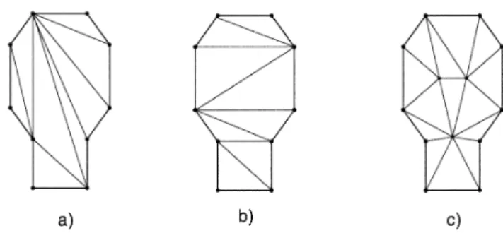
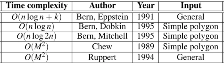
Fig. 1.a)Low quality triangulation; b)High quality triangulation; c)Triangulation with Steiner’s Points. There is a large number of different ways how
to triangulate a given polygon. What all these possibilities have in common is that the number of diagonals isn;3 and the number of the tri-angles being generated isn;2. For details and proofs seeOROU94].
Following the fact of existence of the diagonal, a basic triangulation algorithm can be constructed as follows:
Find a diagonal, cut the polygon into two pieces, and recurs each.
Finding diagonals is a simple task, which is re-peated until all diagonals of the polygon are determined. This can be described as follows:
For every edgeeof the polygon not inci-dent to either end of the potential diagonal s, check if e intersects s. As soon as an intersection is detected, it is known that s is not a diagonal. If no polygon edge intersectss, thensis a diagonal.
A rough analysis shows that such algorithm takes O(n
4
) time. Namely there are n
2
= O(n
2
) diagonal candidates. Testing each of them with all polygon edges costs O(n) time. Repeating this O(n
3
) process for each of the n;3 diagonals gives us an algorithm with at most O(n
4
) running time. Such a direct ap-proach is, of course, too inefficient and therefore many authors proposed much faster triangula-tion algorithms.
There are different possibilities how to triangu-late a given polygon (see Fig. 1). For some applications it is essential that the minimum in-terior angle of a triangle of the computed tri-angulation is as large as possible which defines quality. How the algorithms triangulated a sim-ple polygon depended on the technique used by the algorithm. In Figure 1a for example, the
triangulation can be considered as a low qual-ity, because there are a lot of sliver triangles. The algorithms based on Delaunay triangula-tion ensure better triangulatriangula-tion(Figure 1b). The quality can be significantly improved by using so-called Steiner’s points(Figure 1c).
3. Polygon triangulation algorithms based on diagonal inserting
History of the polygon triangulation algorithms began in 1911LENN11]. In that year Lennes proposed the “algorithm” which worked by re-cursively inserting diagonals between pairs of vertices of P and ran in O(n
2
). At that time mathematicians were interested in constructive proofs of existence of triangulation for simple polygons. Since then, this type of algorithm reappeared in many papers and books. Induc-tive proof for the existence of triangulation was proposed by MeistersMEIS75]. He proposed an ear searching method and then cutting them off. Vertexviof simple polygonPis a principal
vertex if no other vertex ofPlies in the interior of the triangle vi;1, vi, vi+1 or in the interior of the diagonal vi;1, vi+1. A principal vertex vi of simple polygon P is an ear if the
diago-nal vi;1, vi+1 lies entirely in P. We say that two ears vi, vj are non-overlapping if interior
vi
;1 vi vi+1 ]\vj
;1 vj vj+1
] = 0(see Figure 2).
Meisters proved the next theoremMEIS75]: Except for triangles, every simple poly-gon P has at least two non-overlapping ears.
A direct implementation of this idea leads to a complexity of O(n
3
). But in 1990 it was dis-covered that prune and search technique finds an ear in the linear timeGIND93]. It is based on the following observation:
A good subpolygonP1 of a simple poly-gon P is a subpolygon whose boundary differs from that of P in one edge at the most.
The basic observation here is that a good sub-polygonP1has at least one proper ear. Strategy is as follows:
Split the polygonPof n vertices into two subpolygons in O(n) time such that one of these subpolygons is a good subpoly-gon with at mostbn=2c+1 vertices. Each subpolygon is then solved recursively. The worst case running time of the algorithm is T(n)=cn+T(bn=2c+1), wherecis a constant. This recurrence has solutionT(n)2O(n). That leads to implementation of Meisters’s algorithm with the complexity ofO(n
2 ).
Garey, Johnson, Preparata and Tarjan proposed a divide — and — conquer algorithm which first brokeO(n
2
)time complexity(1978)GARE78]. Algorithm runs in O(nlogn) time. Their ap-proach includes two steps: the first one de-composes simple polygon into monotone sub-polygons in O(nlogn). The second step tri-angulates these monotone sub-polygons, which can be done in a linear time. A different divide — and — conquer approach by Chazelle also
achieves O(nlogn) running time CHAZ82]. Very complicated data structures are used in Tarjan and Van Wyk’s algorithm running in O(nlog logn) timeTARJ89]. However, Kirk-patrik introduced an algorithm with the same time complexity but with simple data structures
KIRK90].
Next improvement of speed was gained by algo-rithms with time complexityO(nlog
n). Such algorithms were not just faster but also sim-pler to implement. They all have in common a randomized (“Las Vegas”) approach. The best known algorithm was suggested by Seidel
SEID91]. His algorithm runs in practice almost in linear time for the majority simple polygons. The algorithm has three steps:
trapezoidal decomposition of the polygon, determination of monotone polygon’s chains, and finally,
the triangulation of these monotone poly-gon’s chains.
The efficiency of Seidel’s algorithm is achieved by very efficient trapezoidal decomposition, which works in two steps:
first a random permutation of edges is deter-mined, and
these edges are inserted incrementally into trapezoidal decomposition.
With two corresponding structures containing current decomposition and search structure pre-sented algorithm runs inO(nlog
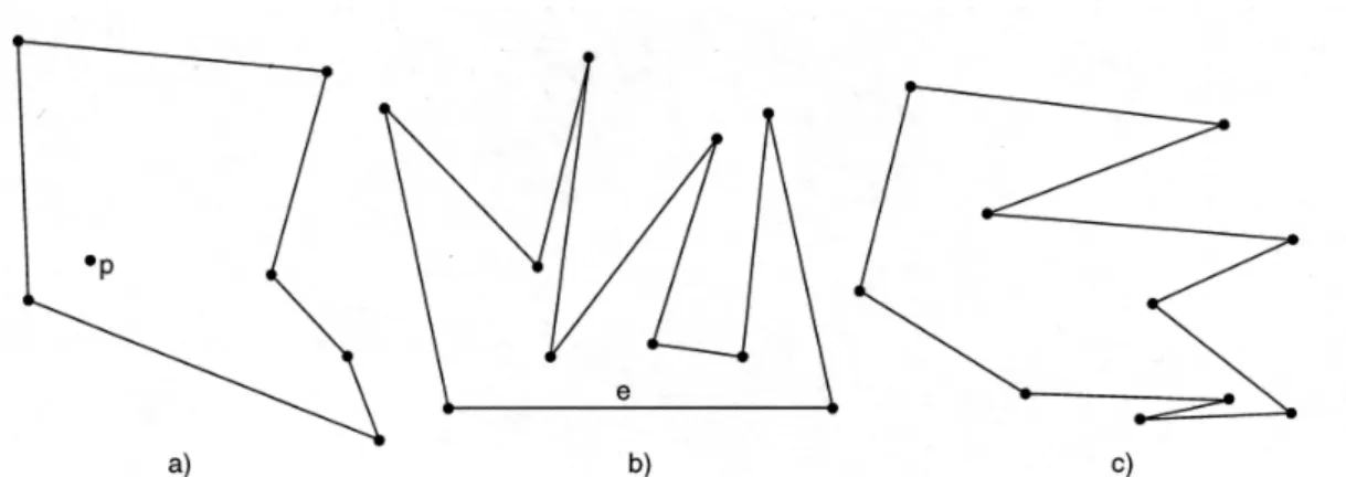
n)time. Researches also searched for classes of poly-gons that can be triangulated in a linear time. They determined that monotone polygons(Fig.
3c), star-shaped polygons (each point in the polygon can be connected to star point p that no edge of polygon boundary is intersected)
(Fig. 3a), spiral polygons,L-convex polygons, edge visible polygons (each point in the poly-gon can be connected to one point of edgeethat no edge of polygon boundary is intersected)
(Fig. 3b), intersection-free polygons and palm-shaped polygons could be triangulated in linear time
Some researches designed adaptive algorithms that run fast in many situations. Hertel and Mehlhorn described a sweep-line based algo-rithm that runs faster if a polygon has fewer concave vertices HERT83]. Algorithm’s run-ning time isO(n+rlogr)whererdenotes the number of concave vertices ofP.
Chazelle and Incerpi also presented algorithm where time complexity depends on shape of the polygonCHAZ84]. They describe a triangula-tion algorithm that runs inO(nlogs)time where s<n. The quantitysmeasures the sinuosity of the polygon representing how many times the polygon’s boundary alternates between com-plete spirals of opposite orientation. In practice, quantitys is very small or a constant, even for very winding polygons. Consider the m otion of a straight line Lvi vi
+1
] passing through edge vi,vi+1where 0
<i<n. Every timeLreaches
the vertical position in a clockwise ( counter-clockwise) manner we decrement (increment) a winding counter by one. Lis spiraling( anti-spiraling)if the winding counter is never decre-mented (incremented) twice in succession. A new polygonal chain is restarted only when the previous chain ceases to be spiraling or anti-spiraling.
Toussaint proposed inTOUS91]another adap-tive algorithm which runs inO(n(1+t0));t0 < n. The quantityt0measures the shape-comple-xity of the triangulation delivered by the algo-rithm. More precisely, t0 is the number of tri-angles contained in the triangulation that share zero edges with the input polygon. The algo-rithm runs in O(n
2
) in the worst case, but for several classes of polygons it runs in the linear time. The algorithm is very simple to imple-ment, because it does not require sorting or the use of balanced tree structures.
Kong, Everett and Toussaint algorithm is based on the Graham scanKONG90]. The Graham scan is a fundamental backtracking technique in computational geometry. It has been shown how to use the Graham scan for triangulating simple polygon in O(kn) time where k ;1 is the number of concave vertices inP. Although the worst case algorithm’s time complexity is O(n
2
), it is easy to be implemented and
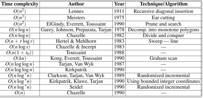
there-Time complexity Author Year Technique/Algorithm
O(n 2
) Lennes 1911 Recursive diagonal insertion
O(n 3
) Meisters 1975 Ear cutting
O(n 2
) ElGindy, Everrett, Toussaint 1990 Prune and search
O(nlogn) Garey, Johnson, Preparata, Tarjan 1978 Decomp. into monotone polygons
O(nlogn) Chazelle 1982 Divide and conquer
O(n+rlogr) Hertel & Mehlhorn 1983 Sweep — line
O(nlogs) Chazelle & Incerpi 1983 —
O(n(1+t0)) Toussaint 1988 —
O(kn) Kong, Everett, Toussaint 1990 Graham scan
O(nlog logn) Tarjan, Van Wyk 1987 —
O(nlog logn) Kirkpatrik 1990 —
O(nlog
n) Clarkson, Tarjan, Van Wyk 1989 Randomized incremental
O(nlog
n) Kirkpatrik, Klawe, Tarjan 1990 Using bounded integer coordinates O(nlog
n) Seidel 1990 Randomized incremental
O(n) Chazelle 1990 —
fore it is useful in practice. The algorithm adapts the Graham scan as following:
The vertices of polygonPare scanned in order starting with v2. At each step the current vertex is tested to determine if it is the top of an ear. If it is not, the current vertex is advanced, otherwise it is an ear and can be cut off. In that case current vertex is not advanced, except for a spe-cial case where the next vertex following cut ear isv0.
Finally, in 1991 Chazelle presentedO(n) worst-case algorithm CHAZ91]. Basic idea is in deterministic algorithm that computes structure called visibility map. This structure is a gener-alization of a trapezoidation(horizontal chords towards both sides of each vertex in a polygonal chain are drawn). His algorithm mimics merge sort. The polygon of n vertices is partitioned into chains with n=2 vertices, and these into chains ofn=4 vertices, and so on. The visibility map of a chain is found by merging the maps of its subchains. This actually takesO(nlogn) time at the most. But Chazelle improves the process by dividing it into two phases. The first phase includes computing coarse approx-imations of the visibility maps. This visibility maps are coarse enough that merging can be ac-complished in a linear time. The second phase refines the coarse map into a complete visibility map, also in the linear time. A triangulation is then produced from the trapezoidation defined by the visibility map. The algorithm has a lot of details and therefore it remains open to find a simple and fast algorithm for triangulating a polygon in the linear time. All mentioned algo-rithms are summarized in Table 1.
4. Polygon triangulation algorithms based on Delaunay triangulation
Triangulation of the simple polygons can also be achieved by the well-known Delaunay triangu-lationFLOR92]on a set of points. Namely, the vertices of a polygon can be considered as indi-vidual input points in the plane. When comput-ing the Delaunay triangulation we have to con-sider that some line segments(edges of poly-gon)must exist at the output. That problem is known as a constrained Delaunay triangulation
(CDT).
Let V be a set of points in the plane and L set of non-intersecting line segments having their extreme vertices at points ofV. The pair G=(V L)defines a constraint graph.
Two verticesPiPj 2 V are said to be mutually visible if either segmentPiPjdoes not intersect
any constraint segment orPiPjis a subsegment
of a constraint segment ofL.
Now the visibility graph of G is a pair Gv =
(Vv Ev);Vv = V andEv =f(Pi Pj)jPi Pj 2 VvandPi Pjare mutually visible with respect
to setLg(see Fig. 4b).
An edge inEv joins a pair of mutually visible
points ofV with respect to all straight-line seg-ments belonging toL.
So, triangulation of V constrained by L is de-fined as a graph T(V;L) = (Vt Et); Vt = V andEtis a maximal subset ofEvLsuch that LEt, and no two edges ofEtintersect, except at their endpoints.
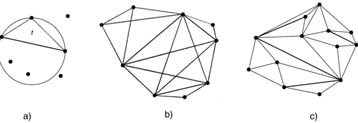
A CDTT(V;L)of set of pointsVwith respect to a set of straight-line segmentsLis a constrained
triangulation ofV in which the circumcircle of each triangle t of T does not contain in its in-terior any other vertex P ofT which is visible from the three vertices of t (see Fig. 4c). An-other characterization of CDT is given by the empty circle property: a triangle t in a con-strained triangulationT is a Delaunay triangle if there does not exist any ot her vertex of T inside the circumcircle oftand visible from all three vertices of t (see Fig. 4a). See details in
FLOR92].
The Delaunay triangulation of simple polygon can be generally computed as follows: the first step computes CDT of edges of simple polygon and the second step removes triangles that are in exterior of simple polygon. The information that input is a simple polygon(not just general constraint graph)could be useful in step one and therefore algorithms for building a CDT can be subdivided into two groups:
algorithms for computing the CDT when the constraint graph is a simple polygon,
algorithms for computing a CDT for general constraint graph.
4.1. Constrained Delaunay triangulation algorithms for simple polygons
Lewis and Robinson described an O(n 2
) al-gorithm based on divide-and-conquer approach with internal points of simple polygonLEWI79]. The boundary polygon is recursively subdivided into almost equally sized subpolygons that are separately triangulated together with their inter-nal points. The resulting triangulation is then optimized to produce CDT.
A recursive O(n 2
) algorithm for CDT based on visibility approach is described by Floriani
FLOR85]. The algorithm computes the visibil-ity graph of the vertices of the simple polygon QinO(n
2
) time and the Voronoi diagramPof set of its vertices in O(nlogn). The resulting Delaunay triangulation is built by joining each vertex Q of P to those vertices that are both visible fromQand Voronoi neighbors ofQ. AnotherO(nlogn)algorithm was described by Lee and Lin in FLOR92]. The algorithm is based on Chazelle’s polygon cutting theorem. Chazelle has shown that for any simple poly-gonPwithnvertices, two verticest1andt2ofP
can be found in a linear time such that segment t1t2 is completely internal to P. Each of the two simple subpolygons resulting from the cut ofP byt1t2 has at leastn=3 vertices. Lee and Lin’s algorithm subdivides the given polygonQ into two subpolygonsQlandQrand recursively
computes the constrained Delaunay triangula-tions Tl and Tr. The resulting triangulationT
of Q is obtained by merging Tl and Tr. They
also proposed a similar algorithm for general constraint graph which runs inO(n
2 ).
4.2. Constrained Delaunay triangulation algorithms for general constraint graphs
Chew describes anO(nlogn)algorithm for the CDT based on the divide-and-conquer approach. The constraint graph G = (V L) is assumed to be contained in a rectangle, which is subdi-vided into vertical strips CHEW87]. In each strip there is exactly one vertex. The CDT is computed for each strip and adjacent strips are recursively merged together. After last merge we got the final CDT. The major problem here is merging those strips that contain edges, which cross some strip having no endpoint in it. Algorithm for computing CDT, which includes preprocessing on the constraint segments, is proposed by Bossiant BOIS88]. By prepro-cessing CDT, the problem is transformed into standard Delaunay problem on a set of points. The idea is to modify the input data by adding points lying on the constraint segments in such a way that resulting Delaunay triangulation is guaranteed to contain such segments. Con-straint segmenteis a Delaunay edge if the circle havingeas diameter does not intersect any other constraint segment. If the circle attached toe intersects some other segment, then e is split into a finite number of subsegments such that none of the circles attached to those segments intersect any constraint. When two constraint segments intersect at an endpoint, one new point is inserted into both segments. The circumcircle of the triangle defined by the common endpoint and by the two new points does not intersect any other constraint segment. This algorithm takes at most O(nlogn) time and generates at most O(n)additional points.
triangulation process. An algorithm proposed by Floriani and PuppoFLOR92]resolves CDT problem by incrementally updating CDT as new points and constraints are added. The problem of incrementally building of CDT is reduced to the following three subproblems:
– computation of an initial triangulation of the domain,
– insertion of a point,
– insertion of a straight-line segment.
An initial triangulation of the domain can be obtained by different approaches. For example, we can determine a triangle or rectangle(made of two triangles), which contain the whole do-main. Then, points and straight-lines are in-crementally inserted. After each insertion we get new CDT which has more elements than the previous one. After inserting the last point or straight-line, the bounding triangle is removed. Algorithm runs at most in O(ln
2
) where n is number of points and lthe number of straight-line segments in the final CDT.
Table 2 shows the algorithms for computing tri-angulation of a simple polygon based on Delau-nay triangulation.
5. Polygon triangulation algorithms by using Steiner points
Finally, the algorithms that care also about the quality of triangulation are considered. The quality is checked regarding the minimum in-terior angle of triangles in the output triangula-tion. Generally, that feature is possible only if the use of so-called Steiner points is allowed.
In that case the number of output triangles is in-creased regarding the minimum number of tri-angles in output triangulation. In other words, we want to provide shape guarantee(minimum interior angle is as high as possible)with mini-mum triangles in the output triangulation(size guarantee).
One of such techniques of triangulation points and straight-lines is Delaunay refinement tech-nique. Chew presented a Delaunay refinement algorithm that triangulates a given polygon into a mesh. In mesh all triangles are between 30 and 120
. The algorithm produces a uniform mesh to obtain all triangles of the roughly the same sizeCHEW89].
Ruppert extended Chew’s work RUPP94] by giving an algorithm such that all triangles in the output have angles between π ;2α. Parame-terα can be chosen between 0 and 20. The triangulation maintained here is a Delaunay tri-angulation set of points which is computed at the beginning. Vertices for Delaunay triangu-lation are in that case endpoints of segments and possible isolated vertices. After comput-ing Delaunay triangulation, vertices are added for two reasons: to improve triangle shape, and to ensure that all input segments are presented in Delaunay triangulation. Two basic opera-tions in the algorithm are splitting a segment by adding a vertex at its midpoint, and splitting a triangle with a vertex at its circumcenter. In each case, the new vertex is added to set of ver-tices. When a segment is split, it is replaced in set of segments by two subsegments. Such algo-rithms runs inO(M
2
)time, whereMis number of vertices at the output, but in practice are very fast.
Time complexity Author Year Input
O(n 2
) Lewis, Robinson 1979 Simple polygon
O(nlogn) Floriani 1985 Simple polygon
O(nlogn) Lee, Lin 1980 Simple polygon
O(n 2
) Lee, Lin 1980 General
O(nlogn) Chew 1987 General
O(nlogn) Boissonnat 1988 General
O(ln 2
) Floriani, Puppo 1992 General
Time complexity Author Year Input O(nlogn+k) Bern, Eppstein 1991 General
O(nlogn) Bern, Dobkin 1995 Simple polygon O(nlog 2n) Bern, Mitchell 1995 Simple polygon
O(M 2
) Chew 1989 Simple polygon
O(M 2
) Ruppert 1994 General
Table 3.Triangulation algorithms based on using Steiner points.
Some other algorithms that give shape guaran-tees are available. They are more complicated to implement and are not based on Delaunay triangulation. Baker BAKE88] has given an algorithm to triangulate the interior of a simple polygon with elements whose angles are be-tween 13
and 90
. The number of triangles used by their algorithm may be unnecessarily large. But they suggested that quadtrees might improve the size of the triangulation. Bern, Eppstein and Gilbert BERN92] followed up this suggestion, as well as giving a new size bound. They showed how to triangulate a pla-nar point set or poligonally bounded domain with triangles of bounded aspect ratio. Trian-gulation has size (number of triangles)within a constant factor of optimal and runs in opti-mal timeO(nlogn+k)with input of sizenand output of size k. Bern, Dobkin, and Eppstein
BERN95]showed how to triangulate polygonal regions with triangles of guaranteed quality. Al-gorithm guarantees, using O(n) triangles, that the smallest height(shortest dimension)of a tri-angle in a triangulation of ann-vertex polygon
(with holes) is a constant factor of the largest possible. Using O(nlogn) triangles for sim-ple polygons(O(n
3=2
)for polygons with holes) they guarantee the largest angle is not greater than 150. Such triangulation can be obtained inO(nlogn)time(O(nlogn+k)for polygons with holes). Another algorithm presented by Bern, Mitchell and RuppertBEMI95] consid-ers triangulation of n-vertex polygonal regions so that no angle in the final triangulation mea-sures more thanπ=2. The number of triangles in the triangulation is only O(n) and the running time is O(nlog
2n
). Algorithm also considers holes in polygons. Basic new technique used in the algorithm is recursive subdivision by disks and consists of two stages: first stage packs the domain with non-overlapping disks, tangent to
each other and to sides of the domain. Disk packing is such that each region not covered has at most four sides. The algorithm then adds edges between ce ntres of disks and points of tangency on their boundaries, thereby dividing the domain into small polygons. Second stage triangulates the small polygons using Steiner points located only interior to the polygons or on the domain boundary.
Table 3 shows algorithms and their time com-plexities described in this section.
6. Common features of groups of algorithms for polygon triangulation
In this section, general properties of all three groups of the algorithms for polygon triangula-tion (algorithms based on diagonal insertion, algorithms based on Delaunay triangulation, and algorithms using Steiner points) are con-sidered. Attributes interesting for comparisons areSHEW]:
quality of a triangulation, number of output triangles, and
the possibility of triangulating polygons with holes.
Figure 5 shows(extended figure fromRUPP94]) how different triangulation is obtained while tri-angulating the same polygon by different algo-rithms:
triangulation in Fig. 5a has been generated by Seidel’s randomized incremental algorithm generates the output in Fig. 5aSEID91]( ba-sed on diagonal inserting),
De Floriani and Puppo’s constrained Delau-nay triangulation generated the Fig. 5b
Fig. 5.a)Diagonal inserting(Seidel); b)Constrained Delaunay triangulation(De Floriani & Puppo); c)Delaunay refinement(Ruppert).
Fig. 5c shows the output of Ruppert’s Delau-nay refinement algorithm RUPP94] (using Steiner points).
It is obvious; the algorithms that use Steiner points achieve the best output triangulation. They have built-in mechanism ensuring the qual-ity of the output triangulation. However, they produced also the larger number of triangles. Delaunay-based algorithms provide the highest quality possible on the original vertices(Fig. 5c). During the construction of the triangulation, they consider so-called Delaunay empty-circle property already mentioned in Section 4. Al-gorithms based on the diagonal insertion do not care at all about the quality of the triangula-tion and because of this, different outputs are obtained by different algorithms(see section 7 where four algorithms from this group are com-pared). However, Delaunay-based algorithms and the algorithms based on diagonal insertion always generate exactly n;2 triangles. If we want to obtain the smallest number of trian-gles possible, and we want to be sure about the quality of the triangulation, then one of the al-gorithms based on Delaunay triangulation has to be used.
The algorithms based on Delaunay triangulation and those using Steiner points handle polygons with holes very easily. They triangulate also the holes, but because we know which edges of the polygon belong to the holes, the triangles inside the holes can be easily removed. The majority of algorithms based on diagonal insertion can-not perform the triangulation of polygons con-taining holes. One of the exceptions is Seidel’s randomized incremental algorithm. Originally, it has not being designed to handle polygons with holes, but it turned out that this extension is very simple. The solution is described in the next section.
7. Comparison of triangulation algorithms based on diagonal insertion
We have already mentioned that the algorithms based on diagonal insertion do not use any cri-teria regarding the quality of the generated tri-angulation and therefore they produce also very different results. This is the reason why in this section some algorithms based on diagonal in-sertion are analyzed.
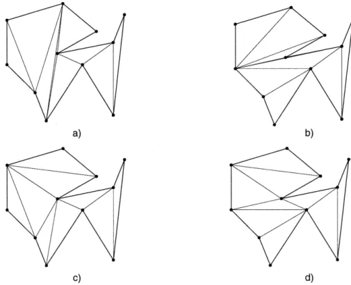
The following algorithms have been chosen: a recursive diagonal inserting algorithmTOUS91], an ear cutting algorithmMEIS75], Kong’s
Gra-ham scan algorithm KONG90], and Seidel’s randomized incremental algorithm SEID91]. All the algorithms have been implemented in C++using the same data structures. Figure 6 shows how different output is generated by these four algorithms.
We tested the speed of the algorithms on two types of polygons: concave polygons and con-vex polygons. We also took concon-vex polygons to determine how fast the algorithms are on poly-gons where triangulation can be obtained in lin-ear time with the simple algorithm(see table 4, column Actual Running Time).
Fig. 6.a)Diagonal inserting; b)Ear cutting; c)Graham scan; d)Randomized incremental.
Actual running time in ms for 5000 points Algorithm Runningtime Averageangle
Convex Concave Holes Recursive diagonal inserting O(n
2
) 3:40
5523 5671 No
Ear cutting O(n
3
) 2:45
10285 10325 No
Kong’s Graham scan O(kn) 4:06
6970 6950 No
Seidel’s rand. Incremental O(nlog
n) 7:94
330 331 Yes
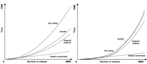
Fig. 7.Speed of algorithms(left — concave polygon; right — convex polygon). Fig. 7 presents the graph showing the running
time of the considered algorithms. For each type of polygons we measured the speed when polygons contain from 3 to 2000 vertices(with step 50). It is clearly seen that Seidel’s random-ized algorithm is in practice the fastest algo-rithm among all compared algoalgo-rithms. Seidel’s algorithm is also not sensitive to on the type of the input polygon. Other three algorithms are considerably slower and their run-time depends on the shape of the input polygon(compare left and right Fig. 7).
As we already said, the algorithms from this group do not contain any mechanism for ensur-ing the quality, and because of different tech-niques used, the algorithms provide different quality of the output triangles. Table 4 shows the average minimum interior angle of obtained triangles for concave polygons with 500 vertices
(test was repeated 100 times on different poly-gons with 500 vertices). Again, the Seidel’s randomized incremental algorithm provides the best result. The reason is that Seidel’s algo-rithms first decompose the input polygon into monotone polygons followed by partitioning of polygons into triangles.
Only Seidel’s algorithm is capable to solve situ-ations when the polygons containing holes are considered(see Table 4, column holes). This is possible because Seidel’s randomized algorithm takes edges randomly on input and builds trape-zoidation. Therefore, we can also add edges of holes on input. After building such
trapezoi-dation we only construct monotone polygons, which are lying in the polygons but not in holes. As shown from Table 4 the Seidel’s algorithm is the best regarding all other three algorithms. The price for this is more complicated imple-mentation.
8. Conclusions
The development of polygon triangulation algo-rithms is still attractive research topic in com-putational geometry. The real challenge is Chazelle diagonal inserting algorithmCHAZ91]. Although theoretically known from 1991, up to now there is no any successful implemen-tation. The new algorithms are still expected among the constraint Delaunay triangulation al-gorithms and especially among the alal-gorithms using Steiner points.
9. Acknowledgement
This work has been carried out within a Valva-sor/ALIS program supported by British Coun-cil(title of the project Computational geometry and its applications in medical visualization).
References
1] B. BAKER, E. GROSSE, C. RAFFERTY Nonobtuse triangulation of polygons.Discrete and Comp. Ge-ometry,3(1988), 147-168.
2] M. BERN, S. MITCHELL, J. RUPPERT Linear-Size Nonobtuse Triangulation of Polygons. Discrete Comput. Geometry,14(1995), 411-428.
3] M. BERG, M. KREVELD, M. OVERMARS, O. SCHWARZKOPF, Computational Geometry, Algo-rithms and Application.Springer Verlog, 1997. 4] M. BERN, D. EPPSTEIN, J. R. GILBERT, Provably
good mesh generation. Presented at the Proceed-ings of the31st Annual Symposium on Foundation
of Computer Science,(1990), 231-241.
5] M. BERN, D. DOBKIN, D. EPPSTEIN, Triangulating polygons without large Angles.Computationl Ge-ometry & Applications,5(1995), 171-192. 6] J. D. BOISSONNAT, Shape reconstruction from
pla-nar cross sections.Comput. Vision Graphics Image Process.,44(1988), 1-29.
7] B. A. CHAZELLE, Theorem on polygon cutting with applications. Presented at the Proceedings of the
23rdIEEE Symposium on Foundation of Computer
Science,(1982), Chicago, 339-349.
8] B. CHAZELLE, J. INCERPI, Triangulation and shape complexity. ACM Transactions on Graphics, 3
(1984), 135-152.
9] B. CHAZELLE, Triangulating a simple polygon in linear time. Discrete Computational Geometry, 6
(1991), 485-524.
10] L. P. CHEW, Constrained Delaunay triangulation. Presented at the Proceedings, Third ACM Sympo-sium on Computational Geometry,(1987), Water-loo, 216-222.
11] L. P. CHEW, Guaranteed — quality triangular meshes. Technical report, No. TR-89-983, Cornell University, 1989.
12] L. DE FLORIANI, B. FALCIDIENO, C. A. PIENOVI, Delaunay-based representation of surfaces defined over arbitrarily-shaped domains. Comput. Vision Graphics Image Processing.32(1985), 127-140. 13] L.DEFLORIANI, E. PUPPO, An On-Line Algorithm
for Constrained Delaunay Triangulation,Graphical Models and Image Processing,3(1992), 290-300. 14] M. R. GAREY, D. S. JOHNSON, F. P. PREPARATA, R.
E. TARJAN, Triangulating a simple polygon,Inform.
Process.,7(1978), 175-180.
15] H. ELGINDY, H. EVERETT, G. T. TOUSSAINT, Slicing an ear in linear time. Pattern Recognition Letters, 14(1993), 719-722.
16] S. HERTEL, K. MEHLHORN, Fast triangulation of simple polygons. Presented at Proceedings4th
In-ternat. Conf. Theory,(1983)pp. 207-215.
17] D. G. KIRKOATRICK, M. M. KLAWE, R. E. TAR
-JAN,O(nlog logn)polygon triangulation with sim-ple data structures. Presented at ACM Symposium on Computational Geometry, 6(1990)pp. 34-43, Berkeley, California.
18] X. KONG, H. EVERETT, G. T. TOUSSAINT, The gra-ham scan triangulates simple polygons. Pattern Recognition Letters,11(1990), 713-716.
19] N. J. LENNES, Theorems on the simple finite polygon and polyhedron.American Journal of Mathematics, 33(1911), 37-62.
20] B. A. LEWIS, J. S. ROBINSO, Triangulating of planar regions with applications. Comput. J., 4 (1979), 324-332.
21] G. H. MEISTERS, Polygons have ears. American
Mathematical Monthly,82(1975), 648-651. 22] J. O’ROURKE,Computational Geometry in C.
Cam-bridge University Press, 1994.
23] J. RUPPERT, A Delaunay Refinemt Algo-rithm for Quality 2-Dimensional Mesh Gen-eration. NASA Arnes Research Center, Sub-mission to Journal of Algorithms, (1994),
http://jit.arc.nasa.gov/nas/abs.html.
24] R. SEIDEL, A simple and fast incremental random-ized algorithm for computing trapezoidal decom-positions and for triangulating polygons. Compu-tational Geometry: Theory and Applications, 1
(1991), 51-64.
25] J. R. SHEWCHUK, Triangle: Engieering a 2D Qual-ity Mesh Generator and Delaunay Triangulator. Carnegie Mellon University,ftp:cs.cmu.edu.
27] G. T. TOUSSAINT, Efficient triangulation of simple polygons.The Visual Computer,7(1991), 280-295. Received:October, 2000
Accepted:November, 2000
Contact address:
Marko Lamot Hermes Softlab Litijska 51 1000 Ljubljana Slovenia Tel:+386 61 1865 815;
Fax:+386 61 1865 816;
e-mail:[email protected]
BorutZalikˇ University of Maribor Faculty of Electrical Engineering and Computer Sciences Smetanova 17
2000 Maribor Slovenia
MARKOLAMOTcurrently works for at Hermes SoftLab computer
com-pany, Ljubljana, Slovenia. He received his BSc in computer engineering in 1996 from the University of Maribor, Slovenia. Currently he is work-ing on his PhD degree at University of Maribor. His research interests include computational geometry especially triangulating algorithms and uniform grids.