http://www.sciencepublishinggroup.com/j/ajomis doi: 10.11648/j.ajomis.20180302.13
ISSN: 2578-8302 (Print); ISSN: 2578-8310 (Online)
Minimizing the Discounted Average Cost Under Continuous
Compounding in the EOQ Models with a Regular Product
and a Perishable Product
Siddharth Mahajan
*, Krishna Sundar Diatha
Production and Operations Management Area, Indian Institute of Management, Bangalore, India
Email address:
*Corresponding author
To cite this article:
Siddharth Mahajan, Krishna Sundar Diatha. Minimizing the Discounted Average Cost Under Continuous Compounding in the EOQ Models with a Regular Product and a Perishable Product. American Journal of Operations Management and Information Systems.
Vol. 3, No. 2, 2018, pp. 52-60. doi: 10.11648/j.ajomis.20180302.13
Received: July 4, 2018; Accepted: July 17, 2018; Published: August 17, 2018
Abstract: We consider the EOQ model with an opportunity cost of capital, i.e. an amount x invested now will yield (1+i)x at
the beginning of the next period. Here i is the interest rate. Given a cost stream i.e. a stream of costs incurred over time, the Net Present Value (NPV) is used to decide the total cost of the cost stream. This total cost takes into account the opportunity cost of capital. The Discounted Average Cost changes the NPV, which is a total, into a cost rate per unit time. The discounted average cost is a cost rate. If we incur this cost rate for the entire period of time under consideration, it will lead to the same NPV as the actual NPV of the cost stream. The discounted average cost under continuous compounding is thus an alternative objective to the standard objective of average cost, which is also a cost rate. We minimize the discounted average cost under continuous compounding for two EOQ models, one with a regular product and the other with a perishable product. Perishable products include food, medicines, certain chemicals and blood in blood banks. In the EOQ model with a perishable product, inventory decays at a constant rate over time. We find the optimal order quantity for the two models while minimizing discounted average cost under continuous compounding.Keywords: Inventory, EOQ Model, Discounted Average Cost, Continuous Compounding, Perishable Product
1. Introduction
The EOQ model is a very widely used and studied inventory model. In the EOQ model we find the order quantity which minimizes average cost. In this paper we consider the EOQ model but with an alternative objective. This objective instead of being the average cost is the discounted average cost under continuous compounding. So we find the order quantity in the EOQ model that minimizes the discounted average cost under continuous compounding.
Background material on continuous compounding and on the discounted average cost is presented in Section 2. We briefly discuss it here. The average cost is an important objective, but it has one drawback. It ignores the time value of money. There is an opportunity cost of capital, i.e. costs incurred now are more expensive than costs incurred later. Given a cost stream i.e. a stream of costs incurred over time,
the Net Present Value (NPV) is used to decide the total cost of the cost stream. This total cost takes into account the opportunity cost of capital.
The Discounted Average Cost changes the NPV which is a total, into a cost rate per unit time. The discounted average cost (of a cost stream) over a specific time interval, is the cost rate that if incurred continuously over the interval, results in the same NPV as the actual cost stream. The NPV is like a total. The discounted average cost is a cost rate. If we incur this cost rate for the entire period of time under consideration, it will lead to the same NPV as the actual NPV of the cost stream. Detailed discussion on the calculation of the discounted average cost is presented in Section 2.
the standard objective that is used. According to Porteus [1], `the discounted average cost can be viewed as an adjustment to the average cost that takes into account the timing of expenditures’. If the bulk of the expenditures occur early in the cost stream, the discounted average cost would go up. Because of the time value of money an early expenditure is more costly than a later expenditure of the same amount. Similarly, if the bulk of expenditures occur later in the cost stream, the discounted average cost would go down.
In this paper, we minimize the discounted average cost under continuous compounding in the EOQ model. Continuous compounding is discussed in Section 2. We also consider the EOQ model with a perishable product. For this model also, we minimize the discounted average cost under continuous compounding.
For a good discussion of the EOQ model, refer Nahmias [2]. The discussion in Section 2 on Discounted Average Cost and Continuous Compounding is based on Porteus [1], Appendix C. The EOQ model with a perishable product is discussed in Section 4 and follows the analysis done in Zipkin [3]. This analysis then becomes the basis for finding the optimal order quantity by minimizing the discounted average cost under continuous compounding for the EOQ model with a perishable product.
Recent work on the EOQ model includes the paper by Ouyang et al [4]. The authors consider an EOQ model for deteriorating items under trade credits. In the EOQ model it is assumed that the supplier is paid immediately after product is received. However, in reality, suppliers may offer a permissible delay as well as a cash discount. Given, this the authors find the optimal policy of the customer to minimize cost.
In other recent work, Tripathy et al [5] consider an EOQ model with process reliability considerations. In the EOQ model it is assumed that the items produced are of perfect quality. However, in reality, product quality is not perfect. The authors consider an EOQ model with an imperfect production process in which the unit production cost is directly related to process reliability.
Eroglu and Ozdemir [6] consider an EOQ model where each lot contains some defective items and shortages are backordered. It is assumed that the entire lot is screened to separate good and defective items. The effect of percentage defective in the lot on the optimal solution is studied and numerical examples are provided.
In Giri et al [7] a single item EOQ model for deteriorating items with a ramp-type demand and Weibull deterioration distribution is considered. Shortages in inventory are allowed and backlogged completely. A numerical solution of the model is obtained, and the sensitivity of the parameters involved in the model is also examined. Salameh and Yaber [8] consider an EOQ model for items of imperfect quality. This paper extends the traditional EOQ model by accounting for imperfect quality items when using the EOQ formulae. This paper also considers the issue that poor-quality items are sold as a single batch by the end of the full screening process. A mathematical model is developed and numerical examples
are provided to illustrate the solution procedure.
Ouyang et al [9] consider the following model. To attract more sales suppliers frequently offer a permissible delay in payments if the retailer orders more than or equal to a predetermined quantity. The authors consider an EOQ model with permissible delay in payment with (1) the retailer’s selling price per unit is significantly higher than unit purchase price, (2) the interest rate charged by a bank is not necessarily higher than the retailer’s investment return rate, (3) many items such as fruits and vegetables deteriorate continuously, and (4) the supplier may offer a partial permissible delay in payments even if the order quantity is less than a predetermined amount. The authors establish the mathematical model, and derive several theoretical results to determine the optimal solution under various situations.
Chua et al [10] also consider an inventory model of deteriorating items under permissible delay in payments. The main purpose of this paper is to investigate the properties of the convexity of the cost function of the inventory model of the deteriorating items under a permissible delay in payments. The paper shows that the cost per unit time is piecewise-convex and a solution procedure is developed.
This paper is organized as follows. In Section 2, we present background on continuous compounding and discounted average cost. In Section 3 we minimize the discounted average cost under continuous compounding in the EOQ model. The standard EOQ Model for a perishable product is considered in Section 4. In Section 5 we consider the EOQ model for a perishable product with discounted average cost under continuous compounding. In Section 6 we discuss a numerical example for the EOQ model with a perishable product. Finally Conclusions are presented in Section 7.
2. Background on Continuous
Compounding and Discounted
Average Cost
The background material in this section is based on Porteus [1], Appendix C, Discounted Average Value.
Consider an n period planning horizon. A stream of costs ct, t=1, 2,..., n is incurred at the beginning of each period. In n is small or the periods are short, we can just add the costs to find the total cost. However, in many cases, we have to consider the time value of money. That is, a dollar invested now is worth more than a dollar invested in the future. This is because instead of investing the dollar, we can put it in a bank account. The $1 dollar will become $(1+i) at the beginning of the second period. Here i is the interest earned on the principal deposited, i.e. $1.
denotes the NPV of the cost stream,
vNPV = ∑t=1n αt-1 ct
If the interest rate i per period is known and if costs occur at the beginning or end of discrete periods, then the NPV can be calculated as above. However if costs occur in the middle of the period or if periods are of different lengths or some costs are incurred continuously over time, then it is difficult to calculate the NPV. In such cases, Continuous Compounding can be a big help.
Consider an annual interest rate i. If interest is compounded once a year, $1 invested at the beginning of the year will yield $(1+i) at the beginning of the second year.
If interest is compounded twice a year (every 6 months) $1 invested at the beginning of the year would yield $(1+i/2)2 at the beginning of year 2. In the same way if interest is compounded m times a year, $1 invested at the beginning of the year would yield $(1+i/m)m at the beginning of year 2. If instead of a year we consider a time period [0,t], over which interest is compounded m times Then $1 invested at the beginning of the time period would yield $(1+it/m)m at the end of the time period.
Continuous Compounding results when m goes to infinity. We use the result,
limm→∞ (1+it/m)m = eit
Then, under continuous compounding, $1 invested at the beginning of the time period [0,t] would yield eit dollars at the end of the time period.
The following Lemma follows Lemma C.1 page 263 of Porteus [1].
Lemma 1:
Suppose that interest is compounded continuously at the rate of i per unit time.
(a)The present value (at time 0) of x dollars received at time t, is xe-it
(b)The present value ( at time 0) of incurring costs at a continuous rate of x dollars per unit time over the time interval [0,t] is x(1 - e-it )/i
Proof:
Part (a) follows from the discussion above. For Part (b), we have
vNPV = ʃτ=0t x e-iτdτ
= x(1 - e-it)/i
Porteus [1] defines the Discounted Average Value (DAV) of a cost stream over a specific time interval, as the cost rate that if incurred continuously over the interval, yields the same NPV as the actual cost stream.
According to Porteus [1], `The DAV simply reexpresses the NPV, which is a total, into a rate of expenditures per unit time. That is, the DAV rescales the net present value into a uniform cost rate’’.
One advantage of the DAV is that it is directly comparable to Average Cost, as we will see in the example below. In
what follows, we would be using the terms `DAV’ and `discounted average cost’ interchangeably, as they are the same. We next have the following Lemma. (Theorem C.1 Porteus [1])
Lemma 2:
Given, vNPV the NPV (as of time 0) of a given cost stream, the equivalent DAV over [0,t] is given by
vDAV = ivNPV/(1 - e-it )
Proof:
Suppose costs are incurred at the rate of vDAV over [0,t]. Then by Lemma 1(b), the resulting NPV is
vNPV = vDAV (1 - e-it )/i
Rearranging the expression above, the result of the Lemma follows.
To illustrate the calculation of the Discounted Average Cost, vDAV, and see that it is comparable to average cost, we use the example below from Porteus [1].
Example:
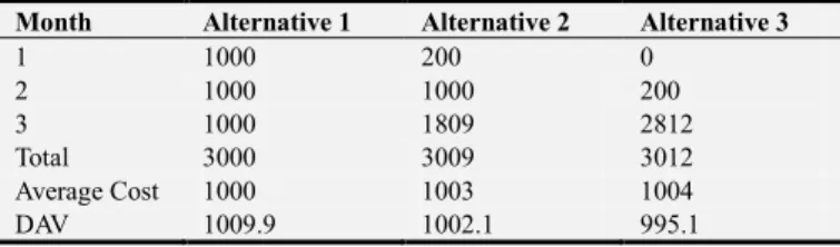
Suppose that interest is compounded continuously at the rate of 2% per month. We face the following 3 alternative cost streams and costs are incurred at the beginning of each month.
Table 1. The Average Cost and DAV for 3 alternative cost streams.
Month Alternative 1 Alternative 2 Alternative 3
1 1000 200 0
2 1000 1000 200
3 1000 1809 2812
Total 3000 3009 3012
Average Cost 1000 1003 1004
DAV 1009.9 1002.1 995.1
Because we are using continuous compounding the effective discount rate is α = e-i (Here t=1) = e-0.02 =0.9802. That is, we need to keep aside only α= e-i dollars at the beginning of the first period to pay $1 at the beginning of the second period.
The discount factor of the costs in the second and third period are respectively, α2 = e-2i =0.9607 and α3 = e-3i = 0.9417
The NPVs as of time 0, for the 3 alternatives are follows: vNPV
vNPV (1) = 1000* e-i + 1000* e-2i + 1000* e-3i =2941.0 vNPV (2) = 200* e-i + 1000* e-2i + 1809* e-3i = 2918.3 vNPV (3) = 0* e-i + 200* e-2i + 2812* e-3i = 2897.7
To compute the DAV for the time interval [0,3], we apply Lemma 2 with i=0.02 and t=3. The factor,
i/(1 - e-it) = 0.3434 So,
vDAV (1) = 0.3434*2941.0 = 1009.9 vDAV (2) = 0.3434*2918.3 = 1002.1 vDAV (3) = 0.3434*2897.7 = 995.1
The above example illustrates the calculation of the DAV. It also shows that DAV is an alternative to average cost and is comparable to average cost.
Approximating the DAV
use the result of this section in later sections. Let O(x) denote an arbitrary function f(x) with the property that limx→0 |f(x)/x| is finite. In particular O(i2) denotes a function that behaves like a constant times i2 when i is small. So if i is close to 0, the ratio of this function to i2 is a constant.
We have the following result from Porteus [1], page 268, Theorem C.2
Theorem 1:
The DAV over the time interval [0,T] for a single expenditure x at time t, can be written as
vDAV = {x+ix(T/2 - t)}/T + O(i2)
Proof:
Here vNPV = xe-it
From Lemma 2, vDAV = ivNPV/(1 - e-iT ) = i(xe-it )/(1 - e-iT )
Let f(i) = (ie-it )/(1 - e-iT ) (1)
We know that f(i) has an expansion of the form a0 + a1i + O(i2),
without yet knowing a0 and a1. Also, e-it = 1- it + (it)2 /2 + O(i3),
From (1), we have
f(i) (1 - e-iT ) = ie-it (2)
We equate the expansions term by term on the LHS and RHS of (2) to find a0 and a1.
From (2), the expansion of the LHS is,
(a0 + a1i + O(i2))( iT - (iT)2 /2 + O(i3))
= i(a0T) + i2(a1T - a0T2 /2) + O(i3) (3)
From (2), the RHS, ie-it, has the expansion
ie-it = i – i2t + O(i3) (4)
Equating (3) and (4) term by term, we have a0T = 1
and a1T - a0T
2 /2 = -t
This gives a0 = 1/T and a1 = (T /2 – t)/T and f(i) ≈ a0+ a1i
= 1/T + i(T /2 – t)/T
Therefore, the approximate DAV for a single expenditure x at time t, is given by
vDAV = ivNPV/(1 - e -iT
) = i(xe-it )/(1 - e-iT ) = xf(i)
≈ x/T + ix(T /2 – t)/T
We will be making use of this result in the following sections.
3. Minimizing the Discounted Average
Cost under Continuous Compounding
in the EOQ Model
In the standard EOQ model we minimize the average cost
over a cycle. In this section, instead of minimizing the average cost we would minimize the discounted average cost in the EOQ model. That is, we would find the order quantity which minimizes the discounted average cost under continuous compounding. Thus we are considering an EOQ model with a different cost function.
Consider an EOQ model with the following costs. The cost of purchasing a product is c per unit. The setup cost for ordering the product from the supplier is K per order. This setup cost is incurred every time the product is ordered. It is independent of the actual quantity ordered.
There is a holding cost, h, for holding the product in inventory. Typically a holding cost consists of two components. One is the direct cost and the other is the financing cost. The direct cost consists of costs for physical handling, insurance, refrigeration and warehouse rental. The financing cost consists of interest payments on capital borrowed to finance the inventory. In this model we assume that the inventory holding cost consists of only the direct cost and not the financing cost. This is a standard assumption in inventory models with discounting or inventory models which take into account the time value of money. See Zipkin [3], pages 34 and 63.
The annual demand in the model is λ units. As in the EOQ model with average cost, in this model also we analyse costs over one cycle of the EOQ model, i.e. the time between receipt of two orders. This cycle repeats itself. We assume that interest is continuously compounded at the rate of i per unit time.
We first consider the purchase cost c and the setup cost K. We next consider the holding cost. Consider one cycle of the EOQ model. Suppose the order quantity is Q. This is the decision variable which we have to find by minimizing the discounted average cost under continuous compounding. At the start of the cycle, we incur the cost K+cQ.
We now use Theorem 1. The DAV over the time interval [0,T] for a single expenditure x at time t, can be written as
vDAV ≈ {x+ix(T/2 - t)}/T
Here x = K+cQ, T = Q/ λ and t=0. Here T is the time for one cycle of the EOQ model to get completed. The DAV over the time interval [0,T] for a single expenditure of K+cQ at time 0 is given by
vDAVs≈ (K+cQ)λ/Q + i(K+cQ)/2
Or vDAVs≈ Kλ/Q + cλ + iK/2 + icQ/2 (5)
We have found the DAV over one cycle for the purchase cost and the setup cost. We next find the DAV over one cycle for the holding cost, vDAVh. We do this by finding, vNPVh, the NPV of the holding cost for one cycle under continuous compounding. We then use Lemma 2 to find vDAVh.
If we plot the inventory over time for the EOQ model, each cycle has a sawtooth pattern. The inventory rises to Q at the start of the cycle and depletes at a constant demand rate λ, till it becomes 0 at the end of the cycle.
be written as,
I(t) = Q – λt
The NPV of the holding cost under continuous compounding,
over one cycle of the EOQ model is,
vNPVh= ʃ0ThI(t)e-itdt
= ʃ0Th(Q – λt)e-itdt (6)
We have,
ʃ0Te-itdt = (1- e-iT )/i (7)
Below, integrating by parts,we have
ʃ0T te-itdt = (-te-it)/i |0T + 1/i ʃ0Te-itd
= 1/i2 - e-iT/ i2 – Te-iT /i (8)
From (6), (7) and (8), we have
vNPVh = hQ(1- e-iT )/i - hλ/i2 + (hλe-iT)/ i2 + (hλTe-iT)/i
= hQ(1- e-iT )/i - hλ/i[(1- e-iT )/i] + (hQe-iT)/I (9)
We now use Lemma 2 to find the DAV under continuous compounding of the holding cost over one cycle of the EOQ model. This is denoted by vDAVh. We have from Lemma 2
vDAVh = ivNPVh /(1 - e-iT )
Substituting (9) for vNPVh, we have that vDAVh is given by
vDAVh = hQ - hλ/i + + (hQe-iT)/(1 - e-iT ) (10)
Combining (5) and (10), we have that the discounted average cost for the EOQ model under continuous compounding, vDAV, is given by
vDAV= vDAVs + vDAVh
= Kλ/Q + cλ + iK/2 + icQ/2
+ hQ - hλ/i + (hQe-iT)/(1 - e-iT ) (11)
We have to find the value of Q which minimizes vDAV. This is different from the standard EOQ model where we minimize average cost. As Example 1 in Section 2 shows, the discounted average cost under continuous compounding is comparable to average cost. It is also an alternative criterion as compared to the average cost.
We can write (11) as
vDAV= Kλ/Q + icQ/2
+ hQ/(1 - e-iT ) + cλ - hλ/i + iK/2 (12)
In the EOQ model, we have that λ is the annual demand and Q is the order quantity in one cycle of the EOQ model. This cycle repeats itself. Typically, the order frequency in a year in the EOQ model, denoted by OF, would be around 15 or 20. That is, the order frequency, OF = λ/Q would be around 15 to 20. So Q/λ = 1/OF would be small. We use this
to get an approximation of one term in the equation (12) for vDAV.
We find an approximation for the term hQ/(1 - e-iT ), where T = Q/ λ.
Let y = Q/ λ, with y small Then,
hQ/(1 - e-iT ) = hλy /(1 - e-iy ) = a0 + a1y + O(y2)
Here we need to find a0 and a1
λhy = [a0 + a1y + O(y2) ][ 1 - e-iy]
= [a0 + a1y + O(y2) ][iy - i2y2/2 + O(y3) ]
Or,
λhy = (a0i)y + [a1i - a0i2/2] y2 + O(y3)
Equating coefficients of y and y2 above, we have
a0i = λh and a1i - a0i2/2 = 0
This gives, a0 = λh/i and a1 = λh/2 So,
hλy /(1 - e-iy ) ≈ a0+ a1y
= λh/i + λhy/2 (13)
Substituting (13) in (12) and using y = Q/λ, we have
vDAV≈ Kλ/Q + icQ/2
+ λh/i + hQ/2 + ( cλ - hλ/i + iK/2 )
= Kλ/Q + icQ/2
+ hQ/2 + ( cλ + iK/2 )
= Kλ/Q + Q/2(h + ic) + cλ + iK/2 (14)
We can now find the value of Q, which minimizes the Discounted Average Cost or vDAV. From (14), the optimal Q which minimizes vDAV is,
Q* = sqrt (2Kλ/h+ic )
This is very similar to the optimal Q in the standard EOQ model with average cost. Thus considering either the average cost or the discounted average cost under continuous compounding in the EOQ model, gives similar results.
4. The Standard EOQ Model for a
Perishable Product
a perishable product.
In the model with a perishable product, we assume that inventory decays at a constant rate over time, independent of its age. If δ is the decay rate and I(t) is the inventory at time t, then inventory deteriorates at rate δI(t) for all t. The defective product is detected immediately and discarded.
We are considering the standard EOQ model with material cost c per unit and the setup cost per order of K. There is a holding cost h per unit per unit time which does not include the financing cost, as discussed in the previous section. Also λ is the annual demand. We consider one cycle of the EOQ model. This cycle repeats itself. Let Q be the inventory ordered at the start of a cycle. Here Q is the decision variable. Assuming time 0 is the beginning of a cycle, we have I(0) = Q
Given our assumption of the decay rate, within a cycle, taking both spoilage and demand into account, we have
I’(t) = - δI(t) – λ (15)
This is a first order differential equation with initial condition, I(0) = Q. Its solution is ( see Zipkin [3] ),
I(t) = Qe-δt - λ/δ( 1- e-δt ) (16)
That equation (16) is the solution of the differential equation (15) can be checked with direct substitution.
The cycle time T, is the value of t with I(t) = 0. Instead of using Q, we use T as the decision variable. Given T, the order quantity Q is given by,
Q = λ/δ( eδT - 1) (17)
The above equation uses I(T) =0.
The average inventory over a cycle, Iavg, is given by (see Zipkin [3] )
Iavg = 1/Tʃ0TI(t)dt
= λ/δ( eδT - δT -1)/ δT (18)
The average cost in the EOQ model with perishable product, C(T), is given by the material cost, the setup cost and the holding cost. It is
C(T) = (K+cQ)/T +hIavg
Using (17) and (18), we have,
C(T) = (K+ c λ/δ( eδT - 1))/T + hλ/δ( eδT - δT -1)/ δT (19)
There is no closed form expression for the optimal cycle time, T. We can solve equation (19), numerically for the optimal T. We can then use equation (17) to find the optimal Q, for the case of the EOQ model with average cost and a perishable product.
5. The EOQ Model for a Perishable
Product with Discounted Average Cost
under Continuous Compounding
In this section, we consider the EOQ model for a
perishable product. We minimize the discounted average cost under continuous compounding, to find the optimal order quantity, Q. We next go about finding the discounted average cost for this case.
We first consider the purchase cost c and the setup cost K. We next consider the holding cost. Consider one cycle of the EOQ model. Suppose the order quantity is Q. This is the decision variable which we have to find by minimizing the discounted average cost under continuous compounding. At the start of the cycle, we incur the cost K+cQ.
We now use Theorem 1. The DAV over the time interval [0,T] for a single expenditure x at time t, can be written as
vDAV ≈ {x+ix(T/2 - t)}/T
Here x = K+cQ and t=0. Here T is the time for one cycle of the EOQ model to get completed. The DAV over the time interval [0,T] for a single expenditure of K+cQ at time 0 is given by
vDAVs≈ (K+cQ)/T + i(K+cQ)/2
Or vDAVs≈ K/T + cQ/T + iK/2 + icQ/2 (20)
From (17) in Section 4, we have that in the case of the EOQ model with a perishable product, Q and T are related as
Q = λ/δ( eδT - 1)
Using the expansion of ex as
ex = 1+ x + x2/2 + O(x3)
and assuming δ small we have that,
Q ≈ λ/δ(δT + δ2T2/2)
= λ(T + δT2/2)
= λT(1 + δT/2) (21)
Substituting (21) in (20), we have
vDAVs≈ K/T + c λ(1 + δT/2) + iK/2
+ (ic/2) λT(1 + δT/2) (22)
We have now found the discounted average cost, vDAVs, resulting from the purchase cost and the setup cost. We next need to find the discounted average cost resulting from the holding cost, i.e. vDAVh. This is similar to the analysis we did in Section 3 for the standard EOQ model.
We do this by finding, vNPVh, the NPV of the holding cost for one cycle under continuous compounding. We then use Lemma 2 to find vDAVh.
The equation for inventory, I(t) as a function of time t for the EOQ model with a perishable product is given by equation (16) in Section 4 as,
I(t) = Qe-δt - λ/δ( 1- e-δt )
vNPVh= ʃ0ThI(t)e-itdt (23)
From the above equation, we have,
I(t) e-it = (Q+ λ/δ)e-(δ+i)t - (λ/δ)e-it (24)
Substituting (24) in (23) and evaluating the integral, we have
vNPVh= (hQ/( δ +i))[ 1- e-(δ+i)T ] – (hλ/δ)[ (1- e-iT)/i]
+ (hλ/δ)[ (1- e-(δ+i)T )/( δ +i) ] (25)
We now use Lemma 2 to find the discounted average cost under continuous compounding of the holding cost over one cycle of the EOQ model. This is denoted by vDAVh. We have from Lemma 2
vDAVh = ivNPVh /(1 - e-iT )
Using (25), we have,
vDAVh = (hQi/( δ +i))[ (1- e-(δ+i)T )/ (1 - e-iT ) ]
hλ/δ
+ ((hλi)/δ( δ +i))[ (1- e-(δ+i)T )/ (1 - e-iT ) ] (26)
Using the expansion of e-x, for x small as
e-x = 1- x + x2/2 + O(x3)
we have
e-x≈ x - x2/2 (27)
We now use (27) in the first term of (26), as δ and i are small. The first term of (26) can be rewritten as,
(hQi/( δ +i))[ (1- e-(δ+i)T )/ (1 - e-iT ) ]
≈ (hQi/( δ +i))[ ( (δ +i)T – ((δ +i)T)2/2 ) / (iT – (iT)2/2 ) ]
= hQ[ ( 1- (δ +i)T/2 ) / (1- iT/2 ) ] (28)
Similarly, we can simplify the third term of (26).
We now substitute (28) in (26) to find the expression for vDAVh. We then have that,
vDAVh≈ hQ[ ( 1- (δ +i)T/2 ) / (1- iT/2 ) ]
- hλ/δ
+ hλ/δ[ ( 1- (δ +i)T/2 ) / (1- iT/2)] (29)
Using the fact that δ and i are small, we have,
( 1- (δ +i)T/2 ) / (1- iT/2 ) ≈ 1 (30)
Using (30) in (29), we have,
vDAVh≈ hQ - hλ/δ + hλ/δ
= hQ
=hλT(1 + δT/2) (31)
In equation (31), we have used equation (21) above.
Combining (22) and (31), we have that the discounted average cost under continuous compounding for the EOQ model with a perishable product, vDAV, is given by
vDAV= vDAVs + vDAVh
≈K/T + cλ(1 + δT/2) + iK/2
+ (ic/2) λT(1 + δT/2)
+ hλT(1 + δT/2) (32)
Rearranging terms of equation (32), we have,
vDAV ≈ K/T + (cλδ/2 +λic/2 + hλ)T
+ (λicδ/4 + hλδ/2)T2
+ (cλ + iK/2) (33)
We can find the value of T which minimizes vDAV. Once we have the optimal value of T, we can find Q using equation (17).
Let a1 = cλδ/2 +λic/2 + hλ
and
a2 = λicδ/4 + hλδ/2
Also let the constant L = cλ + iK/2 Then from equation (33), we have
vDAV ≈ K/T + a1T + a2T2 + L (34)
Let g(T) = K/T + a1T + a2T2 + L
Then, the derivative,
g’(T) = -K/T2 + a1 + 2a2T = 0 (35)
and the second derivative is
g’’(T) = 2K/T3 + 2a2
which is positive.
So the value of T which solves equation (35), i.e. which solves the equation,
a1 + 2a2T = K/T2 (36)
is a point of minima.
We can numerically find the value of T, which solves equation (36). We have thus found the value of T which minimizes the discounted average cost under continuous compounding in the EOQ model with a perishable product.
Once we have T, we can find the optimal order quantity Q for this criterion, using equation (17). In the next section we consider a numerical example for the EOQ model with a perishable product.
6. A Numerical Example for the EOQ
model with a Perishable Product
perishable product, we compare 2 order quantities. The first order quantity is for the standard EOQ model with a perishable product and minimizes average cost. The second order quantity minimizes the discounted average cost under continuous compounding in the EOQ model with a perishable product.
We consider the following numerical example. We have, λ= 1500 units/year, h = $8/unit/year, K = $25 per order c = $25 per unit, δ = i = 0.02
We first consider the standard EOQ model for a perishable product, discussed in Section 4. To find the order quantity, we minimize C(T) in equation (19). Once we have found the optimal T, we can find Q using equation (17).
To find the optimal T in equation (19), we use the fact that δ is small. We expand eδt using the expansion for ex and using δ is small. This gives,
eδT - 1 ≈ δT + (δT)2/2
eδT - δT -1 ≈ (δT)2/2
We substitute these in equation (19) and differentiate to find the best T. Once we have T, we find Q using equation (17). Here again we use that δ is small and expand eδt.
Using the data in the example, this gives T = 0.062 years and Q* = 93.93 for the standard EOQ model for a perishable product.
We next find the optimal Q for the EOQ model for a perishable product for the case of the discounted average cost with continuous compounding. The optimal Q for this criterion has been discussed in the previous section. We first find T and then use equation (17) to find Q.
To find the optimal T, we use equation (36), i.e.
a1 + 2a2T = K/T2
with
a1 = cλδ/2 +λic/2 + hλ
and
a2 = λicδ/4 + hλδ/2
Using the data in the example, we have a1 = 12750 and a2 = 135.
Solving equation (36) in Excel, we have T = 0.0442 years. Using equation (17) this gives Q* = 66.39.
The results of the numerical example are summarized in Table 1 below.
Table 2. Results for the EOQ model for a perishable product.
Q*
Minimize average cost 93.9
Minimize discounted average cost under continuous compounding 66.3
Thus we find that in this numerical example, minimizing discounted average cost under continuous compounding gives a lower order quantity than in the case of the standard EOQ model, which minimizes average cost.
7. Conclusion
The EOQ model minimizes average cost and does not take into account the time value of money. However, the discounted average cost under continuous compounding takes into account the time value of money. Just like the average cost is a cost rate, the discounted average cost is also a cost rate. We find the order quantity in the EOQ model, for the alternative criteria of minimizing discounted average cost under continuous compounding.
For the EOQ model with a regular product, minimizing the discounted average cost under continuous compounding, results in an order quantity which is very similar to the order quantity resulting from minimizing the EOQ model with average cost.
For the EOQ model with a perishable product, a closed form solution for the optimal order quantity is not available for the standard objective of average cost. For the EOQ model with a perishable product and the objective of minimizing discounted average cost, we were not able to obtain a closed form solution. However the optimal order quantity can be easily found numerically. We considered a specific numerical example for the EOQ model with a perishable product. Here we have two objectives, the average cost and the discounted average cost. We found that the order quantity while minimizing discounted average cost under continuous compounding was lower. It remains to be seen, if this numerical result holds more generally.
References
[1] Porteus, E. L. Foundations of Stochastic Inventory Theory, 2002, Stanford University Press: Stanford, California. [2] Nahmias, S. Production and Operations Analysis, 1989, Irwin:
Boston, MA.
[3] Zipkin, P. Foundations of Inventory Management. 2000. McGraw Hill Higher Education.
[4] Ouyang, L. Y., C. T. Chang and J. T. Teng (2005). An EOQ model for deteriorating items under trade credit. Journal of the Operational Research Society. Vol. 56, No. 6, 719-726. [5] Tripathy, P. K., W. M. Wee and P. R. Majhi (2003). An EOQ
model with process reliability considerations. Journal of the Operational Research Society. Vol. 54, No. 5, 549.
[6] Eroglu, A. and G. Ozdemir (2007). An economic order quantity model with defective items and shortages. International Journal of Production Economics. Vol. 106, No. 2, 544-549.
[7] Giri, B. C., A. K. Jalan and K. S. Chaudhuri (2003). Economic Order Quantity model with Weibull deterioration distribution, shortage and ramp-type demand. International Journal of Systems Science. Vol. 34, No. 4, 237-243.
[9] Ouyang, L. Y., J. T. Teng, S. K. Goyal and C. T. Yang (2009). An Economic Order Quantity model for deteriorating items with partially permissible delay in payments linked to order quantity. European Journal of Operational Research. Vol. 194, No. 2, 418-431.