All about A Minimal Normal Form for DNA Expressions

(1)

Technical Report 2011-03

July 2011

Universiteit Leiden

Leiden Institute of Advanced Computer Science

All about a Minimal Normal Form

for DNA Expressions

Rudy van Vliet

[email protected]

Leiden Institute of Advanced Computer Science

Leiden University

(2)

(3)

Technical Report 2011-03

July 2011

Universiteit Leiden

Leiden Institute of Advanced Computer Science

All about a Minimal Normal Form

for DNA Expressions

Rudy van Vliet

[email protected]

Leiden Institute of Advanced Computer Science

Leiden University

(4)

(5)

Preface

In the summer of 2011, Rudy van Vliet and Hendrik Jan Hoogeboom prepared a paper entitled “A minimal normal form for DNA expressions”, and submitted it to the scientific journalFundamenta Informaticae. As the title suggests, this paper presented a minimal normal form for DNA expressions. Moreover, it described an algorithm to rewrite an arbitrary DNA expression into the normal form. This is a two-step algorithm: it first rewrites the DNA expression into an equivalent, minimal DNA expression, and then rewrites the result of that into the normal form.

In the summer of 2012, after the paper had been reviewed by the journal, it was splitted into two papers, allowing for more detailed proofs of the results. The first paper, entitled “Making DNA expressions minimal”, describes the first step of the two-step algorithm, i.e., the algorithm to rewrite an arbitrary algorithm into an equivalent, minimal DNA expression. The second paper, entitled “A minimal normal form for DNA expressions”, describes the minimal normal form and an algorithm to rewrite an arbitrary minimal DNA expression into the normal form. The two new papers are self-contained. They were submitted together, as a diptych, to Fundamenta Informaticae, and were accepted for publication.

The interested reader of the papers may wish to see more details. Therefore, we compiled this report. In contains even more detailed proofs of the results from the papers (including auxiliary results, again with proofs), more examples illustrating the text and a section with a related topic that is not covered in the papers (§ 7.4).

The following table may serve as a quick reference list from definitions, examples, results, table and figures in the papers to their equivalents in this report:

In paper 1 In paper 2 In report

Definition 1 Definition 2.5

DNA expression Definition 2.11

Theorem 2 Theorem 3.3

Theorem 3 Theorem 1 Theorem 5.3

Definition 4 Definition 2a Definition 4.3, Definition 5.4 Definition 5 B↓(X),B↑(X) Definition 4.5

Definition 6 Definition 2b Definition 5.8, Definition 5.9

Example 3 Example 5.14

Theorem 7 Theorem 4 Theorem 5.12

Example 8 Example 5 Example 5.14

Example 9 Lemma 6.14(2)

Theorem 10 Theorem 6 Lemma 6.15, Theorem 6.16

Lemma 11 Lemma 7 Lemma 7.21

Example 12 not in this report

Lemma 13 Theorem 7.20

(8)

Example 17 not in this report

Lemma 18 Lemma 7.34

Lemma 19 Lemma 7.36

Theorem 20 Theorem 7.37, Corollary 7.38, Theorem 7.40

Definition 8 Definition 8.1

Theorem 10 Lemma 8.6, Lemma 8.7, Theorem 8.8

language of minimal

normal form is regular § 8.4

Theorem 15 Theorem 9.10, Theorem 9.12

Figure 1 Figure 1 Figure 5.4

Table 1 Table 6.1

Figure 2 Figure 7.1, Figure 7.15

Figure 3 Figure 7.3

Figure 4 Figure 7.4

Figure 5 Figure 4 Figure 7.5

Figure 6 Figure 7.16, Figure 7.17, Figure 7.18

Figure 2 Figure 9.1

Figure 3 Figure 9.4, Figure 9.6

This report was first published in July 2011. This preface is the only part of the report that has been adjusted since then.

Rudy van Vliet October 2012

(9)

Abstract

DNA expressions consitute a formal language/notation for DNA molecules that may contain nicks and gaps. Different DNA expressions may denote the same DNA molecule. We define a (minimal) normal form for this lan-guage and describe an algorithm to rewrite a given DNA expression into the normal form.

(10)

(11)

Chapter 1 Introduction

In the past two decades, DNA computing has become a flourishing research area. Since [Head, 1987] and [Adleman, 1994], researchers from various disciplines, ranging from theoretical computer science to molecular biology, investigate the computational power of DNA molecules, both from a theoretical and an experimental point of view. Nowa-days, research groups from all over the world contribute to the field, see, e.g., [Deaton & Suyama, 2009] and [Sakakibara & Mi, 2011]. Current topics of interest include, a.o., gene assembly in ciliates, DNA sequence design, self-assembly and nanotechnology, see, e.g., [Ehrenfeucht et al., 2004], [Kari et al., 2005], [Winfree, 2003], [Reif, 2003], [Rothemund, 2006] and [Chen et al., 2006]. The basic concepts of DNA computing are described in [Paun et al., 1998].

Despite the growing interest in DNA computing, not much attention is paid in literature to formal ways to denote the DNA molecules – exceptions are [Boneh et al., 1996] and [Li, 1999]. Formal notations can, however, be useful, e.g., to precisely denote molecules and to compactly describe the computations carried out using them.

In [Van Vliet, 2004], [Van Vliet et al., 2005] and [Van Vliet et al., 2006], we have introducedDNA expressions as a formal notation for DNA molecules that may contain nicks (missing phosphodiester bonds between adjacent nucleotides in the same strand) and gaps (missing nucleotides in one of the strands). Different DNA expressions may denote the same DNA molecule. Such DNA expressions are calledequivalent. In these three publications, it is also explained how to constructminimal DNA expressions: the shortest possible DNA expressions denoting a given molecule.

When one wants to decide whether or not two DNA expressions E1 and E2 are

equivalent, one may determine the DNA molecules that they denote and check if these are the same. In this report, we present a different approach. We define anormal form: a set of properties, such that for each DNA expression there is exactly one equivalent DNA expression with these properties. We also describe an algorithm to rewrite an arbitrary DNA expression into the normal form. Now to decide whether or not E1

and E2 are equivalent, one determines their normal form versions and then checks if

these are the same. This approach is elegant, because it operates at the level of DNA expressions only, rather than to refer to the denoted DNA molecules.

The report is organized as follows. In Chapters 2–6, we recall a number of definitions and results which we have published before and which we need for the normal form and the algorithms. In particular, in Chapter 2, we introduce the concepts of a formal DNA molecule and a DNA expression. Chapter 3 contains some results on DNA expressions in general. Chapter 4 deals with (lower bounds on) the length of a DNA expression.

(12)

2 Ch. 1 Introduction

In Chapter 5, we describe how to construct minimal DNA expressions. In Chapter 6, we find out that there do not exist minimal DNA expressions other than the ones constructed in Chapter 5.

For every known definition or result in Chapters 2–6, we mention the corresponding definition or result in the earlier publications. We do not repeat the proofs for the old results, as they can simply be looked up, especially in [Van Vliet, 2004]. In addition, these five chapters contain some new, related results. For those, we do provide the proofs.

Because the contents of Chapters 2–6 are meant mainly as background material, we have not put much effort in presenting it as a nice, fluent story. This is different for Chapters 7–9, which describe the normal form and the algorithms.

In Chapter 7, we present an algorithm to rewrite an arbitrary DNA expression into an equivalent, minimal DNA expression. By itself, this is not sufficient to yield a normal form. For many DNA molecules, there exist many (equivalent) minimal DNA expressions. Depending on the input, the algorithm may yield each of these. However, the algorithm can function as a first step towards a true normal form.

Such normal form is introduced in Chapter 8. As the DNA expressions that satisfy the normal form are minimal, it is called a minimal normal form. In Chapter 9, we describe an algorithm for constructing this normal form. It first uses the algorithm from Chapter 7 to construct a minimal DNA expression, and then rewrites the result into the minimal normal form. This turns out to be more efficient than an alternative, direct algorithm.

(13)

Chapter 2 Terminology and Notation

2.1 Strings,

N

_{-words, trees, grammars and}

com-plexity

An alphabet is a finite set, the elements of which are called symbols or letters. A finite sequence of symbols from an alphabet Σ is called a string over Σ. For a string X =x1x2. . . xr over an alphabet Σ, with xi ∈Σ for i = 1,2, . . . , r, the length of X is

r and it is denoted by |X|. The length of the empty string λ equals 0.

For a non-empty string X = x1x2. . . xr, we define L(X) = x1 and R(X) = xr.

The concatenation of two strings X1 and X2 over an alphabet Σ is usually denoted by

X1X2; sometimes, however, we will writeX1·X2.

The set of all strings over an alphabet Σ is denoted by Σ∗_{, and Σ}+ _{= Σ}∗_{\ {}_λ_}_(the

set of non-empty strings). A language over Σ is a subset K of Σ∗.

LetN ={A, C, G, T}be the alphabet of nucleotides. The elements ofN are called

N-letters. We reserve the symbol a (possibly with a subscript) to denote N-letters. A non-empty string over N is called an N-word. Clearly, the set N+ _of _N_{-words is}

closed under concatenation. We reserve the symbol α (possibly with a subscript) to denote N-words.

Substrings

A substring of a stringX is a (possibly empty) string Xs _{such that there are (possibly}

empty) stringsX1 andX2withX =X1XsX2. IfXs6=X, thenXsis aproper substring

of X. We call the pair (X1, X2) an occurrence of Xs in X. If there exists a (possibly

empty) string X2 such that X = XsX2, then Xs is a prefix of X; if there exists a

(possibly empty) string X1 such thatX =X1Xs, thenXs is a suffix ofX. If a prefix

of X is a proper substring of X, then it is also called aproper prefix. Analogously, we may have a proper suffix of X.

If (X1, X2) and (Y1, Y2) are different occurrences ofXs inX, then (X1, X2)precedes

(Y1, Y2) if |X1| < |Y1|. Hence, all occurrences in X of a given string Xs are linearly

ordered, and we can talk about the first, second, . . . occurrence of Xs _{in X. Although,}

formally, an occurrence of a substringXs _{in a string}_X _{is the pair (X}

1, X2) surrounding

Xs _in _{X, the term will also be used to refer to the substring itself, at the position in}

X determined by (X1, X2).

Note that for a string X = x1x2. . . xr of length r, the empty string λ has r+ 1

occurrences: (λ, X),(x1, x2. . . xr), . . . ,(x1. . . xr−1, xr),(X, λ).

(14)

4 Ch. 2 Terminology and Notation

IfXs ₌_a _{for a letter} _a_{from the alphabet Σ, then the number of occurrences of}_Xs

in X is denoted by #a(X). Obviously, when X = x1x2. . . xr with x1, x2, . . . , xr ∈ Σ,

#a(X) is the number of xi’s that are equal to a. Sometimes, we are not so much

interested in the number of occurrences of one letter in a string X, but rather in the total number of occurrences of two different letters aand b inX. This total number is denoted by #a,b(X).

If a string X is the concatenation of k times the same substring Xs_{, hence} _X ₌

Xs. . . Xs

| {z }

ktimes

, then we may writeX in the form (Xs₎k_.

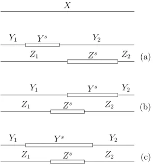
Let (Y1, Y2) and (Z1, Z2) be occurrences in a string X of substrings Ys and Zs,

respectively. We say that (Y1, Y2) and (Z1, Z2) are disjoint, if either |Y1|+|Ys| ≤ |Z1|

or |Z1|+|Zs| ≤ |Y1|. Intuitively, one of the substrings occurs (in its entirety) before

the other one.

If the two occurrences are not disjoint, hence if |Z1| < |Y1| + |Ys| and |Y1| <

|Z1|+|Zs|, then they are said to intersect. Note that, according to this formalization

of intersection, an occurrence of the empty string λ may intersect with an occurrence of a non-empty string. For example, in the string X = ACATGAT over the alpha-bet N, the third occurrence of λ (the occurrence (AC,ATGAT)) intersects with the (only) occurrence of CAT. In the remainder of this report, however, we will not come across intersections ofλ with other strings. Occurrrences of two non-empty substrings intersect, if and only if the substrings have at least one (occurrence of a) letter in common.

We say that (Y1, Y2) overlaps with (Z1, Z2), if either |Y1| < |Z1| < |Y1 +|Ys| <

|Z1|+|Zs|or|Z1|<|Y1|<|Z1|+|Zs|<|Y1|+|Ys|. Hence, one of the substrings starts

before and ends inside the other one.

Finally, the occurrence (Y1, Y2) ofYs contains (orincludes) the occurrence (Z1, Z2)

of Zs_{, if}_|_Y

1| ≤ |Z1| and |Z1|+|Zs| ≤ |Y1|+|Ys|.

If it is clear from the context which occurrences of Ys _and _Zs _in_X _{are considered,}

e.g., if these strings occur inX exactly once, then we may also say that the substrings Ys _and _Zs _themselves _{are disjoint, intersect or overlap, or that one contains the other.}

Note the difference between intersection and overlap. If (occurrences of) two sub-strings intersect, then either they overlap, or one contains the other, and these two possibilities are mutually exclusive For example, in the string X = ACATGAT over

N, the (only occurrence of the) substringYs _{= ATGA intersects with both occurrences}

of the substring Zs _{= AT. It contains the first occurrence of} _Zs _{and it overlaps with}

the second occurrence of Zs_.

In Figure 2.1, we have schematically depicted the notions of disjointness, intersec-tion, overlap and inclusion.

Functions on strings

Let Σ be an alphabet. A function h from Σ∗ to a set K with an operation ◦ is called ahomomorphism if h(X1X2) =h(X1)◦h(X2) for all X1, X2 ∈Σ∗. Hence, to specify h

if suffices to give its values for the letters from Σ.

The empty string λ is theidentity 1Σ∗ of Σ∗, i.e., the element satisfying X◦1_Σ∗ = 1Σ∗◦X = X for all X ∈ Σ∗. It follows from the definition of a homomorphism that h(λ) = 1K, where 1K is the identity of K.

(15)

2.1 Strings, N_{-words, trees, grammars and complexity} ₅

X

Y1 Ys Y2

Z1 Zs Z2 _(a)

Y1 Ys Y2

Z1 Zs Z2 _(b)

Y1 Ys Y2

Z1 Zs Z2 _(c)

Figure 2.1: Examples of disjoint and intersecting occurrences (Y1, Y2) of Ys and

(Z1, Z2) of Zs in a string X. (a) The occurrences are disjoint: |Y1|+|Ys| ≤ |Z1|. (b)

The occurrences overlap: |Z1|<|Y1|<|Z1|+|Zs|<|Y1|+|Ys|. (c) The occurrence of

Ys _{contains the occurrence of}_Zs_: _|_Y

1| ≤ |Z1| and |Z1|+|Zs| ≤ |Y1|+|Ys|.

Indeed, |λ|= 0, which is the identity for addition of numbers.

If a homomorphism h maps the elements of Σ∗ _{into Σ}∗ _{(i.e., if} _K _{= Σ}∗ _{and the}

operation is concatenation), then h is called an endomorphism.

The symbolcwill denote the complement function. It is an endomorphism on N∗_,

specified by

c(A) = T, c(C) = G, c(G) = C, c(T) = A.

Thus, for an N-word α,c(α) results by replacing each letter of α by its Watson-Crick complement. For example, c(ACATG) = TGTAC.

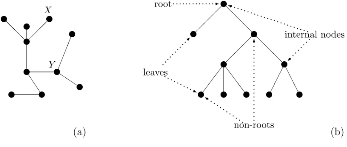
Directed trees

A tree is a non-empty graph such that for all nodes X and Y in the graph, there is exactly one path between X and Y. In particular, a tree is connected. Figure 2.2(a) shows an example of a tree. The distance between two nodes in a tree is the number of edges on the path between the two nodes. For example, the distance between nodes X and Y in the tree from Figure 2.2(a) is 3.

(16)

6 Ch. 2 Terminology and Notation v v v v v v v v v v J J @ @ @ Q Q Y X (a) v v v v v

v v v v v

@ @ @ @ @ @ S S S A A A -... k . . . . . . . . . . . . 6 .. .. .. .. .. .. .. .. .. .. . i . . . . . . . . . . . . . . . . . . . . . . . . . . . . . . . . ... ... j ..._.... root non-roots internal nodes leaves (b)

Figure 2.2: Examples of trees. (a) A tree with ten nodes. (b) A directed tree with ten nodes, in which the root and some non-roots, internal nodes and leaves have been indicated.

partition the nodes in a directed tree: either in a root and non-roots, or in leaves and internal nodes.

Usually, in a picture of a directed tree, the root is at the top, its children are one level lower, the children of the children are another level lower, and so on. An example is given in Figure 2.2(b). In this example we have also indicated the root and some of the non-roots, internal nodes and leaves.

Alevel of a directed tree is the set of nodes in the tree that are at the same distance from the root of the tree. The root is at level 1, the children of the root are at level 2, and so on. The height of a directed tree is the maximal non-empty level of the tree. Obviously, this maximal level only contains leaves. For example, the height of the tree depicted in Figure 2.2(b) is 4, level 2 contains a leaf and an internal node, and level 4 contains five leaves.

It follows immediately from the definition that the height of a tree can be recursively expressed in the heights of its subtrees:

Lemma 2.1 Lett be a directed tree, and let X1, . . . , Xn for somen ≥0 be the children

of the root of t.

1. If n = 0 (i.e., if t consists only of a root), then the height of t is 1.

2. If n ≥1, then the height of t is equal to

n

max

i=1 (height of the subtree of t rooted at Xi)+ 1.

A directed tree isordered if for each internal nodeX, the children ofX are linearly ordered (‘from left to right’). Finally, an ordered, directed, node-labelled tree is an ordered directed tree with labels at the nodes.

Grammars

(17)

2.1 Strings, N_{-words, trees, grammars and complexity} ₇

Acontext-free grammar is a 4-tupleG= (Σ,∆, P, S), where Σ is the total alphabet (the set of all symbols that may occur in an intermediate or final string in the grammar), ∆ is the alphabet ofterminal symbols(the set of symbols that may occur in the elements of the language described),P is a finite set of productions (rewriting rules for elements from Σ\∆) and S is theaxiom (the initial symbol). The elements of Σ\∆ are called non-terminal symbols. Every production is of the formA−→Z, where A∈Σ\∆ and Z ∈ Σ∗_{. It allows for rewriting the non-terminal symbol} _A _{into the string} _Z _{over Σ}

(which may contain both terminal and non-terminal symbols).

Let (X1, X2) be an occurrence of the non-terminal symbol A in a stringX over Σ.

Hence, X =X1AX2. When we apply the production A−→ Z to this occurrence of A

in X, we substituteA in X byZ. The result is the string X1ZX2.

A string that can be obtained from the axiom S by applying zero or more produc-tions from P, is called a sentential form. In particular, the string S (containing only the axiom) is a sentential form. It is the result of applying zero productions.

The language of G (or the language generated by G) is the set of all sentential forms that only contain terminal symbols, i.e., the set of all strings over ∆ that can be obtained from the axiom S by the application of zero or more1 _{productions. We use}

L(G) to denote the language of G.

A languageK is called context-free, if there exists a context-free grammar G such that K=L(G).

Let X be an arbitrary string over Σ. A derivation in G of a string Y from X is a sequence of strings starting with X and ending with Y, such that we can obtain a string in the sequence from the previous one by the application of one production from P. If we use X0, X1, . . . , Xk to denote the successive strings (with X0 = X and

Xk = Y), then the derivation is conveniently denoted as X0 =⇒ X1 =⇒ · · · =⇒ Xk.

If the initial string X in the derivation is equal to the axiom S of the grammar, then we often simply speak of a derivation of Y (and not mention S).

For arbitrary stringsX over Σ, the language LG(X) is the set of all strings over ∆

that can be derived inGfromX: LG(X) = {Y ∈∆∗ |there exists a derivation of Y in

G fromX}. If the grammarG is clear from the context, then we will also writeL(X). In particular, L(G) = LG(S) = L(S).

Example 2.2 Consider the context-free grammar G = ({S, A, B, a, b},{a, b}, P, S), where

P ={S −→ λ

S −→ ASB

A −→ a

B −→ b }.

A possible derivation in G is

S =⇒ ASB

=⇒ aSB

=⇒ aASBB

=⇒ aaSBB

=⇒ aaBB

=⇒ aabB

=⇒ aabb.

(2.1)

1

(18)

In this derivation, we successively applied the second, the third, the second, the third, the first, the fourth and once more the fourth production from P.

It is not hard to see that L(G) ={am_bm _|_m_≥₀_}_.

The notation

A −→ Z1 | Z2 | . . . | Zn

is short for the set of productions

A −→ Z1

A −→ Z2

... ... ...

A −→ Zn

For example, the set of productions from the grammarGin Example 2.2 can be written as

P ={S −→ λ | ASB

A −→ a

B −→ b }.

With this shorter notation for the productions, we will often use ‘production (i, j)’ to refer to the production with the jth _{right-hand side from line} _{i. In our example,}

production (1,2) is the production S −→ASB.

If a sentential form contains more than one non-terminal symbol, then we can choose which one to expand next. Different choices usually yield different derivations, which may still yield the same final string.

Example 2.3 LetGbe the context-free grammar from Example 2.2. Another deriva-tion of the string aabb in Gis

S =⇒ ASB

=⇒ AASBB

=⇒ AASBb

=⇒ aASBb

=⇒ aASbb

=⇒ aaSbb

=⇒ aabb.

(2.2)

If, in each step of a derivation, we expand the leftmost non-terminal symbol, then the derivation is called the leftmost derivation. Derivation (2.1) of aabb in our example context-free grammar is the leftmost derivation,

A right-linear grammar is a special type of context-free grammar, in which every production is either of the from A−→ λ or of the form A −→aB with A, B ∈Σ\∆ and a ∈ ∆. Hence, a production A −→ aB allows for rewriting the non-terminal symbol A into a terminal symbola followed by a non-terminal B.

A language K is called regular, if there exists a right-linear grammar G such that

K=L(G).

(19)

2.2 Formal DNA molecules 9

formal language theory, stating that a language generated by a context-free grammar with a particular property is regular.

Let G be a context-free grammar, let ∆ be the set of terminal symbols in G and let A be a non-terminal symbol in G. We say that A is self-embedding if there exist non-empty strings X1, X2 over ∆, such that the string X1AX2 can be derived from

A. Intuitively, we can ‘blow up’ A by rewriting it into X1AX2, rewriting the new

occurrence of A intoX1AX2, and so on.

Gitself is called self-embedding, if it contains at least one non-terminal symbol that is self-embedding. In other words: Gis not self-embedding, if none of its non-terminal symbols is self-embedding. Clearly, a right-linear grammar is not self-embedding. Hence, any regular language can be generated by a grammar that is not self-embedding. As was proved in [Chomsky, 1959], the reverse is also true: a context-free grammar that is not self-embedding generates a regular language. We thus have:

Proposition 2.4 A language K is regular, if and only if it can be generated by a context-free grammar that is not self-embedding.

Complexity of an algorithm

Analgorithm is a step-by-step description of an effective method for solving a problem or completing a task. There are, for example, a number of different algorithms for sorting a sequence of numbers. In this report, we describe a few algorithms to transform a given DNA expression into another DNA expression with some desired properties. In each of these cases, the input of the algorithm is a DNA expression E, which is in fact just a string over a certain alphabet, satisfying certain conditions.

Algorithms can, a.o., be classified by the amount of time or by the amount of memory space they require, depending on the size of the input. In particular, one is often interested in the time compexity (or space complexity) of an algorithm, which expresses the rate by which the time (space) requirements grow when the input grows. In our case, the size of the input is the length |E| of the DNA expression E. Hence, growing input means that we consider longer strings E.

For example, an algorithm is said to have linear time complexity, if its time re-quirements are roughly proportional to the size of its input: when the input size (the length|E|) grows with a certain factor, the time required by the algorithm grows with roughly the same factor. In this case, we may also say that this time is linear in the input size. An algorithm has quadratic time complexity, if its time requirements grow with a factor c2 _{when the input size grows with a factor}_c.

In the analysis of complexities, we will also use the big O notation. For example, we may say that the time spent in an algorithm for a given DNA expression E is in O(|E|). By this, we mean that this time grows at most linearly with the length

|E| of E. In this case, in order to conclude that the algorithm really has linear time complexity, we need to prove that |E|also provides a lower bound for the growth rate.

2.2 Formal DNA molecules

(20)

denote a base pair – two complementary nucleotides that are connected through a hy-drogen bond. In the formal semantics of our DNA expressions, a pair of corresponding elements in the upper strand and the lower strand is denoted by a composite symbol

x = x

+

x−

. Here x+ _{stands for the nucleotide in the upper strand and} _x− _{stands for}

the nucleotide in the lower strand. If we happen to have a gap in either of the strands, the missing nucleotide is denoted by −. Hence, x+_{, x}− _{∈ N ∪ {−}}_{. For convenience,}

we will speak of a base pair also if one of two complementary nucleotides is missing. If both nucleotides are present, we may call the base paircomplete.

Of course, the value of x+ _{restricts the value of} _x−_{, and vice versa. Because of}

the Watson-Crick complementarity and the fact that a missing nucleotide cannot face another missing nucleotide, only 12 out of the 25 possible composite symbols x

+

x−

are really allowed: A_T

, C_G

, G_C

, _AT

, A₋

, ₋C

, G₋

, T₋

, −_A

, −_C

, −_G

, −_T

. The set of these 12 composite symbols is denoted by A.

For the future use, we partitionA into three subsets: A± =

n _A

T

, _GC

, G_C

, T_A

o,

A+ =

n _A

−

, ₋C

, G₋

, T₋

o and A− =

n ₋

A

, −_C

, −_G

, −_T

o. The elements of A

are called A-letters, the elements of A± are called double A-letters, the elements of

A+ are called upper A-letters, and the elements of A− are called lower A-letters.

Consequently, a non-empty string overAis called anA-word, a non-empty string over

A± is called a double A-word, a non-empty string over A+ is called anupper A-word,

and a non-empty string over A− is called a lowerA-word.

We also need symbols to denote nicks. There are three possibilities for the connec-tion structure of two adjacent base pairs in a double stranded DNA molecule: there can be a nick in the upper strand, there can be a nick in the lower strand, or there can be no nick at all between the base pairs. Note that there cannot be both a nick in the upper strand and a nick in the lower strand between two adjacent base pairs. In such a situation, there would be no connection whatsoever between the base pairs, so they would be parts of different DNA molecules.

The case that there is no nick at all is the default; it is not denoted explicitly. A nick in the upper strand is denoted by ▽

and a nick in the lower strand by △. We call ▽

and △the nick letters – ▽

is theupper nick letter, and △ the lower nick letter. Now, a complete description of a linear DNA molecule possibly containing nicks and gaps can be given by a non-empty string X over A▽△ =A ∪ {

▽ ,△}.

Definition 2.5 (See [Van Vliet, 2004, Definition 2.1], [Van Vliet et al., 2005, Definition 1], [Van Vliet et al., 2006, Definition 1]) A formal DNA molecule is a string X =x1x2. . . xr with r≥1 and for i= 1, . . . , r, xi ∈ A▽△, satisfying

1. if xi ∈ A+, then xi+1 ∈ A/ − (i= 1,2, . . . , r−1),

if xi ∈ A−, then xi+1 ∈ A/ + (i= 1,2, . . . , r−1),

2. x1, xr ∈ A,

3. if xi ∈ {

▽

,△}, then x_i₋₁, x_i₊₁ ∈ A_± (i= 2,3, . . . , r−1).

(21)

2.2 Formal DNA molecules 11

x+_i and upper nick letters in X as the upper strand of X. The lower strand of X is defined analogously.

If a formal DNA molecule does not contain upper nick letters, then we say that its upper strand is nick free. Similarly, if a formal DNA molecule does not contain lower nick letters, then its lower strand is nick free. If a formal DNA molecule does not contain nick letters at all, then the molecule is called nick free.

When we build up a formal DNA molecule from left to right, the choice of a certain letter completely determines the possibilities for the next letter. For example: a nick letter must be succeeded by a double A-letter; an upper A-letter may be succeeded by either an other upperA-letter or a doubleA-letter, or it may terminate the formal DNA molecule (see Definition 2.5). With this in mind, it is easy to construct a right-linear grammar that generates the language F. We thus have:

Lemma 2.6 The language F of formal DNA molecules is regular.

Components of a formal DNA molecule

LetX =x1. . . xr be a formal DNA molecule, withxi ∈ A▽△ fori= 1, . . . , r. Aformal DNA submolecule ofX is a substringXs _of_X _{such that}_Xs _{is a formal DNA molecule.}

It is easy to see that

Lemma 2.7 A substring Xs _{of a formal DNA molecule} _X _{is a formal DNA molecule}

if and and only if |Xs_{| ≥}₁ _and _L(Xs_{), R(X}s₎_{∈ A}_.

Definition 2.8 (See [Van Vliet, 2004, Definition 2.3], [Van Vliet et al., 2005, Definition 2], [Van Vliet et al., 2006, page 130])LetX be a formal DNA molecule. Then the decomposition ofX is the sequencex′₁, . . . , x′k ofk ≥1non-empty strings over

A▽△ such that

• X =x′

1. . . x′k,

• for i = 1, . . . , k, x′

i is either an upper A-word, or a lower A-word, or a double

A-word, or a nick letter, and

• for i= 1, . . . , k−1, if x′

i is an upper A-word, then x′i+1 is not an upper A-word,

and similarly for lower A-words and double A-words.

Hence, the decomposition of X cannot be simplified any further. For the ease of notation, we will in general write x′

1. . . x′k instead of x′1, . . . , x′k.

Ifx′

1. . . x′k for somek ≥1 is the decomposition of a formal DNA molecule X, then

the substrings x′i are called the components of X. For i = 1, . . . , k, if x′i is an upper

A-word (lowerA-word or doubleA-word), thenx′

i is called anupper component (lower

component or double component, respectively) of X. If x′

i is not a double component,

then we may also call it a non-double component of X. Upper components and lower components of X are also called single-stranded components of X.

Corollary 2.9 (See [Van Vliet, 2004, Corollary 2.5]) LetX be a nick free formal DNA molecule and let x′₁. . . x′_k for some k ≥1 be the decomposition of X.

1. For i = 1, . . . , k, x′i is either an upper component, or a lower component, or a

(22)

2. Fori= 1, . . . , k−1,

• if x′

i is a single-stranded component, then x′i+1 is a double component, and

• if x′

i is a double component then x′i+1 is a single-stranded component.

2.3 Properties, relations and functions of formal

DNA molecules

Properties

LetX =x1. . . xr be a formal DNA molecule, withxi ∈ A▽△ fori= 1, . . . , r. Then the upper strand of X is said to cover the lower strand to the right if R(X) = xr ∈ A/ −,

hence, if x+

r 6=−; note that, since xr is not allowed to be a nick letter (condition 2 of

Definition 2.5),x+

r is well defined. Intuitively, the upper strand extends at least as far

to the right as the lower strand then.

If R(X) = xr ∈ A+, hence x−r = − (the upper strand extends even beyond the

lower strand to the right), then the upper strandstrictly covers the lower strand to the right. In an analogous way we can define ‘(strict) covering to the left’.

Of course, the definition of ‘(strict) covering’ can also be formulated for the lower strand.

Relations

We say that a formal DNA molecule X1 prefits a formal DNA molecule X2 by upper

strands, denoted by X1⊏X2, if the upper strand of X1 covers the lower strand to

the right and the upper strand of X2 covers the lower strand to the left, hence, if

R(X1) ∈ A/ − and L(X2) ∈ A/ −; we also say that X1 is an upper prefit for X2 then.

Intuitively, when we write X1 and X2 after each other in such a case, the respective

upper strands ‘make contact’.

Analogously, we defineX1 toprefit X2 by lower strands (to be alower prefit forX2)

if R(X1)∈ A/ + and L(X2)∈ A/ +, and write then X1⊏X2. If either X1⊏X2 or X1⊏X2,

we say that X1 prefits X2 or thatX1 is a prefit for X2, and write then X1 ⊏X2.

IfX1 prefitsX2 (by upper/lower strands), then, from the perspective ofX2, we say

that X2 postfits X1 (by upper/lower strands), or that X2 is an (upper/lower) postfit

for X1.

If the order of the formal DNA molecules is clear, then we may also say that X1

and X2 fit together (by upper/lower strands).

Functions

We define four endomorphisms on the setA∗

▽△: ν

+_, _ν−_, _ν _and _{κ. Let} _x_{∈ A}

▽△. Then

ν+(x) =

x if x∈ A ∪ {△}

λ if x=▽ (2.3)

ν−(x) =

x if x∈ A ∪ {▽

}

λ if x=△ (2.4)

ν(x) =

x if x∈ A

λ if x∈ {▽

(23)

2.4 Operators and DNA expressions 13

κ(x) =

    

x if x∈ A±∪ {▽,△}

a c(a)

if x= ₋a

for a∈ N

c(a)

a

if x= −_a

for a∈ N

(2.6)

It is easy to see (by inspecting the effect of the functions on the symbols fromA▽△), that applying the same function more than one time, does not change the result:

h(h(X)) =h(X) for each h∈ {ν+, ν−, ν, κ}and X ∈ A∗

▽△. (2.7)

For example, ν(ν(X)) =ν(X) for each X∈ A∗

▽△.

Lemma 2.10 (See [Van Vliet, 2004, Lemma 2.7])For each formal DNA molecule X,

L(ν+(X)) =L(ν−(X)) = L(ν(X)) =L(X), R(ν+(X)) =R(ν−(X)) =R(ν(X)) =R(X), L(κ(X)), R(κ(X))∈ A±.

2.4 Operators and DNA expressions

The formal DNA molecules constitute the foundation of our DNA language. They allow us to define the elements of the DNA language: the DNA expressions.

The basic building blocks of DNA expressions are N-words. DNA expressions result by applying operators toN-words. The operators we consider in this report are

↑, ↓ and l, to be pronounced as uparrow, downarrow and updownarrow, respectively. DNA expressions also contain opening and closing brackets: h and i, which delimit the scope of the operators – each (occurrence of an) operator acts only on the part of the expression that is contained between its opening and closing brackets. Hence, the set of all DNA expressions, denoted by D, is a language over the alphabet ΣD, where

ΣD =N ∪ {↑,↓,l,h,i}={A,C,G,T,↑,↓,l,h,i}.

We will use the symbol E (possibly with annotations like subscripts) to denote a DNA expression. If a string can be either an N-word or a DNA expression, then we use ε (possibly with annotations like subscripts) to denote it.

Informally, a DNA expression is a string of the form h↑ε1ε2. . . εni, h↓ε1ε2. . . εni

orhlε1i, wheren ≥1 and theεi’s are eitherN-words or DNA expressions themselves.

The εi’s are called the arguments of the operator involved. We say that an operator is

applied to its arguments. The arguments of the operators↑ and↓ must satisfy certain conditions, which will be explained shortly.

Clearly, not every string over ΣD is a DNA expression. In particular, every DNA

expression contains brackets and at least one operator, which implies that N-words are not DNA expressions.

(24)

SD

↑

C

G AT GCCG

▽ E

= CATGC

G CG S

D

↑

A

T TA

E

= AT TA△

(a)

SD

↓

T CATGC

G CG

AT TA△

E

= CATGCAT

TG CGTA

▽

(b)

SD

l

CATGCAT

TG CGTA

▽ E

= ACATGCAT TGTACGTA

▽

(c)

Figure 2.3: (See [Van Vliet, 2004, Figure 2.5], [Van Vliet et al., 2005, Fig-ure 1], [Van Vliet et al., 2006, FigFig-ure 1]) Examples of the effects of the three operators. (a) The effect of the operator ↑. (b) The effect of the operator ↓. (c) The effect of the operator l.

The operator ↑can have an arbitrary number n≥1 of arguments. Each argument εi (i= 1,2, . . . , n) must be either anN-wordα, or a DNA expression E. The resulting

DNA expression is h↑ε1ε2. . . εni.

From the molecular point of view, the effect of the operator ↑ is threefold: (1) it produces upper strands corresponding to arguments that are N-words α (as in the basic DNA expressionh↑αi), (2) it repairs all nicks occurring in the upper strands of its arguments by establishing the missing phosphodiester bonds and (3) it fixes such connections between the upper strands of consecutive arguments. In short, ↑connects all pairs of adjacent nucleotides in the upper strands of its arguments.

The third type of effect imposes a (semantical) restriction on the arguments of

↑: consecutive arguments must prefit each other by upper strands. Otherwise, there would be a gap in the upper strand ‘between’ two arguments, and we would not be able to connect the upper strands. Since we have defined ‘prefitting each other by upper strands’ only for formal DNA molecules and for DNA expressions, we consider an N-word α here as the DNA expression h↑αi, which represents the upper A-word

α

−

.

The three types of effect of ↑ are illustrated by the first example in Figure 2.3(a). Nicks that are present in the lower strands of the arguments are not repaired by the operator ↑. As a matter of fact, ↑ introduces nicks between the lower strands of consecutive arguments if these consecutive arguments happen to prefit each other by lower strands, i.e., if they have a blunt edge at each other’s side. The second example in Figure 2.3(a) shows such a situation.

The operator↓is the dual of↑. It can have an arbitrary numbern≥1 of arguments, with each argument εi (i = 1, . . . , n) being either an N-word or a DNA expression.

The resulting DNA expression is h↓ε1ε2. . . εni.

The effect of this operator is similar to that of↑; the only difference is that the roles of the upper strands and the lower strands of the arguments are changed. Consequently, also the requirement on consecutive arguments is changed: for i = 1,2, . . . , n−1, εi

must prefit εi+1 by lower strands. Here, when an argument εi is an N-word α, it is

interpreted as the DNA expression h↓αi, which denotes the lower A-word −_α

. The effect of ↓ is illustrated by Figure 2.3(b).

Unlike the other two operators, l can have only one argument ε1. It is either an

N-word or an (arbitrary) DNA expression. The resulting DNA expression is hlε1i.

Ifε1 is a DNA expression E, then, intuitively, in the DNA molecule denoted by E,

(25)

establishes phosphodiester bonds between the nucleotides added and their respective neighbours in the strand. Hence, it does not introduce new nicks. On the other hand, if the DNA molecule denoted by E has nicks already, then these nicks are not repaired by l. The effect of this operator is illustrated in Figure 2.3(c).

Definition 2.11 (See [Van Vliet, 2004, Definition 2.8 and Definition 2.9], [Van Vliet et al., 2005, pages 378-380], [Van Vliet et al., 2006, pages 131-133]) A DNA expression is a string in any of the following forms:

• h↑ε1ε2. . . εni,

where n ≥ 1, for i = 1,2, . . . , n, εi is either an N-word or a DNA expression,

and for i= 1,2, . . . , n−1, S+_(ε

i)⊏S+(εi+1), where the functionS+ is defined by

S+(ε) =

( _α

−

if ε is an N-word α

S(ε) if ε is a DNA expression . (2.8)

Further,

S(h↑ε1ε2. . . εni) =ν+(S+(ε1))y1ν+(S+(ε2))y2. . . yn−1ν+(S+(εn)) (2.9)

with

yi =

      

△ if S+(ε_i)⊏S+(ε_i₊₁), i.e., if both R(S+(ε_i))∈ A_± and L(S+_(ε

i+1))∈ A±

λ otherwise, i.e., if either R(S+_(ε

i))∈ A+

or L(S+_(ε

i+1))∈ A+ (or both)

(i= 1,2, . . . , n−1).

(2.10)

• h↓ε1ε2. . . εni,

where n ≥ 1, for i = 1,2, . . . , n, εi is either an N-word or a DNA expression,

and for i= 1,2, . . . , n−1, S−_(ε

i)⊏S−(εi+1), where the functionS− is defined by

S−(ε) =

−

α

if ε is an N-word α

S(ε) if ε is a DNA expression . (2.11)

Further,

S(h↓ε1ε2. . . εni) =ν−(S−(ε1))y1ν−(S−(ε2))y2. . . yn−1ν−(S−(εn))

with

yi =

      

▽

if S−_(ε

i)⊏S−(εi+1), i.e., if both R(S−(εi))∈ A±

and L(S−_(ε

i+1))∈ A±

λ otherwise, i.e., if either R(S−_(ε

i))∈ A−

or L(S−_(ε

i+1))∈ A− (or both)

(26)

• hlε1i,

where ε1 is either an N-word or a DNA expression.

Further,

S(hlε1i) =κ(S+(ε1)).

for the function S+ _{defined above.}

Example 2.12 (See [Van Vliet, 2004, Equation (2.17)]) (Cf. [Van Vliet et al., 2005, Equation (4)], [Van Vliet et al., 2006, Equation (4)]) The DNA expression

E =h↓Th↑ hlCiATh↓ hlGi hlCiii h↑ hlAi hlTiii,

uses all three operators. It is easily verified that E denotes the DNA molecule from Figure 2.3(b).

We call a DNA expression of the form h↑ε1. . . εni an ↑-expression, one of the form

h↓ε1. . . εni a ↓-expression, and one of the form hlε1i an l-expression. Hence, the

DNA expression in Example 2.12 is a ↓-expression.

Theorem 2.13 (See [Van Vliet, 2004, Theorem 2.10]) Let E = h↑ε1. . . εi0−1

εi0. . . εj0εj0+1. . . εnibe a DNA expression where for i= 1, . . . , i0−1, j0+ 1, . . . , n, εi is

either an N-word or a DNA expression, and for i= i0, . . . , j0, εi =αi is an N-word.

Let α = αi0. . . αj0. Then S(E) is the same, regardless of the interpretation of α as

one argument or as a sequence of separate arguments αi0, . . . , αj0.

By the above, we are free to interpret consecutiveN-words in a DNA expression as one

N-word. This motivates the definition of a maximalN-word occurrence in a string X (e.g., a DNA expression E) as an occurrence (X1, X2) of an N-word α inX such that

(1) ifX1 6=λ thenR(X1)∈ N/ and (2) if X2 6=λ thenL(X2)∈ N/ . Hence, the N-word

α ‘cannot be extended either to the left or to the right’.

Additional terminology

We say that an operatorgovernsits argument(s) and everything inside its argument(s). In every DNA expression we can identify an outermost operator. This is the operator which has been performed last. It governs the entire DNA expression.

Because of the 1–1 correspondence between a DNA expression and its outermost operator, we will sometimes interchange the terms. In particular, we may speak of the arguments of a DNA expression, while we actually mean the arguments of the outer-most operator of a DNA expression. For example, the (three) arguments of the DNA expression from Example 2.12 are T,h↑ hlCiATh↓ hlGi hlCiiiand h↑ hlAi hlTii. We call (an occurrence of) an operator in a DNA expression E which is not the outermost operator, an inner occurrence of this operator inE.

An operator may occur more than once in a DNA expression. To denote a specific occurrence of an operator, we may provide the operator with an index. For example, we may have↑0 or↓1.

ADNA subexpressionEs _{of a DNA expression}_E _{is a substring of}_E _{which is itself a}

(27)

the outermost operator of a proper DNA subexpression of E is an inner occurrence of this operator in E.

We will use the term ↑-subexpression of E to refer to a DNA subexpression of E which is an ↑-expression. Analogously, we may have a ↓-subexpression and an l -subexpression of E.

For every N-word α occurring in a DNA expression E and for every proper DNA subexpression Es _of _E _{we define its} _{parent operator} _{to be the operator which has}

the N-word or DNA subexpression as an immediate argument. For example, in the DNA expression from Example 2.12, the parent operator of the N-word AT is the first occurrence of the operator ↑ in the DNA expression; for the second occurrence of the

N-word C it is clearly the operator l standing in front of it; and the parent operator of the DNA subexpression hlGi is the second occurrence of the operator ↓.

An occurrence of an operator is an ancestor operator of an N-word or a DNA subexpression ε occurring inE, if ε is contained in an argument of the operator. For example, the ancestor operators of the second occurrence of theN-word C in the DNA expression from Example 2.12 are: the first occurrence of ↓ (the outermost operator), the first occurrence of ↑, the second occurrence of↓ and the third occurrence of l(the parent operator of C).

If an argument of a certain (occurrence of an) operator is anN-word, then we may call it an N-word-argument of the operator. If, on the other hand, the argument is a DNA expression, then we may call it an expression-argument of the operator. In particular, if it is an↑-expression, then we may call it an↑-argument. In an analogous way, we define a ↓-argument and an l-argument of an operator. At some point in this report, it will be useful to have a single term for arguments that are not l-expressions, i.e., for N-word-arguments, ↑-arguments and ↓-arguments. We call such arguments non-l-arguments.

We say that an↑-expression or a↓-expressionE isalternating, if its arguments are maximalN-word occurrences and DNA expressions, alternately. Because by definition, a maximal N-word occurrence cannot be preceded or succeeded by another N -word-argument, this is equivalent to saying that E does not have consecutive expression-arguments. An occurrence of an operator ↑ or ↓ is alternating, if the corresponding DNA subexpression is alternating. Examples of alternating DNA expressions are

E1 = h↑α1i,

E2 = h↑ hlα1ii,

E3 = h↓ h↑α1hlα2iiα3α4hlα5ii,

E4 = h↓α1h↓ hlα2i h↑ hlα3iα4iii.

Both E1 and E2 have exactly one argument, and are by definition alternating. The

N-word-arguments α3 and α4 of E3 together form a maximal N-word occurrence.

This makes E3 alternating. Finally, E4 is alternating, although its second argument

h↓ hlα2i h↑ hlα3iα4ii is not alternating. The ↓-expression in Example 2.12 is not

al-ternating, because both its second argument h↑ hlCiATh↓ hlGi hlCiii and its third argument h↑ hlAi hlTii are DNA expressions.

Let E be a DNA expression, and let α1, . . . , αk for some k ≥ 1 be the maximal

N-word occurrences in E, in the order of their occurrence from left to right. Then we will sometimes write E as a function of these maximal N-word occurrences, hence E =E(α1, . . . , αk). Clearly, α1, . . . , αk also show up in the corresponding formal DNA

(28)

Note, however, that different maximal N-word occurrences αi in E may occur in

the same component of S(E). Moreover, if the parent operator of a maximal N-word occurrence αi is ↓ (which implies that a lower A-word _α−

i

is introduced into the semantics), then this lowerA-word may be complemented by an occurrence ofl. This would result in a double A-word c(_ααi)

i

. Hence, the component of S(E) in which a maximalN-word occurrenceαi ofE appears, is not necessarily an element of WA(αi)

For example, if E =E(α1, α2) =hl h↓α1hlα2iii, thenS(E) = c_α(α1)α2

1c(α2)

.

2.5 Nesting level of the brackets

The brackets in a DNA expression determine a structure with different levels. An opening bracket h corresponds to an increase of the level by 1, a closing bracket i to a decrease of the level by 1. The resulting levels are called the nesting levels of the brackets.

Initially, before the first letter of a DNA expression, the nesting level is 0. Since every opening bracket precedes the corresponding closing bracket, the nesting level is non-negative at any position in a DNA expression. Further, because the number of opening brackets equals the number of closing brackets, the nesting level is back at 0 at the end of a DNA expression.

The maximal nesting level of a DNA expression is of particular interest. For exam-ple, the maximal nesting level of the DNA expression from Example 2.12 is 4.

A DNA expression consists of an opening bracket, an operator, one or more argu-ments and a closing bracket. Hence, the nesting level structure of a DNA expression is determined by the nesting level structure of its arguments. In particular, the maximal nesting level of a DNA expression is determined by the maximal nesting levels of those arguments that are DNA expressions themselves:

Lemma 2.14 Let E be a DNA expression and let E1, . . . , Er for some r ≥ 0 be the

expression-arguments of E.

1. If r = 0 (i.e., if E only has N-word-arguments), then the maximal nesting level of E is 1.

2. If r≥1, then the maximal nesting level of E is equal to

r

max

j=1 (maximal nesting level of Ej)+ 1.

Of course, in the expression in Claim 2, the expression-arguments Ej are viewed as

independent DNA expressions, which start at level 0.

2.6 The functions

L

and

R

for arguments of DNA

expressions

An important requirement on the argumentsε1, . . . , εn of an↑-expression (or↓

-expres-sion) is that they must fit together by upper strands (lower strands, respectively). The requirement for ↑-expressions can be expressed formally in terms of R(S+_(ε

i))

and L(S+_(ε

(29)

2.7 A context-free grammar for D ₁₉

arguments of an operator fit together by upper strands, then we are not interested in the complete semantics of these arguments. Therefore, it would be desirable if we could computeL(S+_(ε

i)) andR(S+(εi)) for anN-word or DNA expressionεiwithout having

to compute S+_(ε

i) explicitly. Actually, we only need to know which of the subsets

A+, A− and A± the A-letters L(S+(εi)) and R(S+(εi)) belong to. For consecutive

arguments εi and εi+1, both R(S+(εi)) and L(S+(εi+1)) must be inA+∪ A±.

Of course, to check if the argumentsε1, . . . , εnof an operator↓fit together by lower

strands, we need to answer a similar question for L(S−_(ε

i)) andR(S−(εi)). Note that

if εi is a DNA expression Ei, then S+(εi) = S−(εi) = S(Ei). Hence, in that case,

L(S+_(ε

i)) =L(S−(εi)) and R(S+(εi) =R(S−(εi)).

We can use the following result to recursively determine the subsets thatL(S+_(ε

i)),

R(S+_(ε

i)),L(S−(εi)) andR(S−(εi)) are an element of:

Lemma 2.15 (See [Van Vliet, 2004, Lemma 2.16]) Let εi be an N-word or a

DNA expression.

1. If εi is an N-word α, then

L(S+_(ε

i)), R(S+(εi))∈ A+,

L(S−(εi)), R(S−(εi))∈ A−.

2. If εi is an l-expression, then

L(S+_(ε

i)) =L(S−(εi)) =L(S(εi))∈ A±,

R(S+(εi)) = R(S−(εi)) =R(S(εi))∈ A±.

3. If εi is an ↑-expression h↑εi,1. . . εi,mi for some m ≥ 1 and N-words and DNA

expressions εi,1, . . . , εi,m then

L(S+_(ε

i)) =L(S−(εi)) =L(S(εi)) =L(S+(εi,1)),

R(S+_(ε

i)) = R(S−(εi)) =R(S(εi)) =R(S+(εi,m)).

4. If εi is a ↓-expression h↓εi,1. . . εi,mi for some m ≥ 1 and N-words and DNA

expressions εi,1, . . . , εi,m then

L(S+(εi)) =L(S−(εi)) =L(S(εi)) =L(S−(εi,1)),

R(S+_(ε

i)) = R(S−(εi)) =R(S(εi)) =R(S−(εi,m)).

2.7 A context-free grammar for

D

As we have established in Lemma 2.6, the language F of formal DNA molecules is regular. This is not the case with the language D of all DNA expressions. This is intuitively clear from the fact that every DNA expression contains matching brackets h

(30)

Lemma 2.16 The language D of DNA expressions is not regular.

Proof: Let α be an arbitrary N-word. Then E1 = hlαi is a DNA expression, and

S(E1) = _c₍α_α₎

. By definition, also E2 = hl hlαii is a DNA expression, with the

same semantics. Using induction, one can easily prove that for arbitrary l ≥ 1, El =

hllα il is a DNA expression, with S(El) = _c₍α_α₎

. By the pumping lemma for regular languages, a language requiring brackets to match and containing such DNA expressions is not regular.

The languageDis, however, context-free, because it can be generated by a context-free grammar. We will give such a grammar, here. It is a 4-tuple G1 = (Σ1,∆1, P1, S1),

which is based on three types of non-terminal symbols: E (which denotes a DNA expression), U (a sequence of one or more arguments of an ↑-expression) and L (a sequence of one or more arguments of a↓-expression).

The crucial issue in the construction of a context-free grammar generating D, is that we must somehow incorporate the requirement that consecutive arguments of an operator ↑ or ↓ fit together by upper strands or lower strands, respectively. For this, the non-terminal symbolsE,U and Lhave two subscripts. The first subscript denotes whether or not one of the strands of the (sub)molecule represented by the non-terminal has to cover the other strand to the left. If it is +, then the upper strand must cover the lower strand to the left; if it is −, then the lower strand must cover the upper strand to the left; if it is ⋆, then it does not matter if either strand strictly covers the other strand to the left. The second subscript has the same meaning, however, with respect to covering to the right. For example, the symbol U+,− denotes a sequence of

arguments of↑, for which the upper strand (of the first argument) must cover the lower strand to the left, and the lower strand (of the last argument) must cover the upper strand to the right.

In addition to the above,G1has one more non-terminal symbol: α, which represents

an arbitrary N-word. We thus have the following set of non-terminal symbols:

{Ex,y, Ux,y, Lx,y |x, y ∈ {⋆,+,−}} ∪ {α}.

The axiom is S1 =E⋆,⋆, which denotes a DNA expression without restrictions on the

two strands. The alphabet ∆1 of terminal symbols is equal to ΣD: ∆1 ={A,C,G,T,↑

,↓,l,h,i}.

Before we present the productions in G1 (i.e., the elements of P1) we discuss why

we have exactly those productions.

We first consider the productions for (rewriting) a non-terminal symbol Ex,y with

x, y ∈ {⋆,+,−}, which represents a DNA expression.

By Lemma 2.15(2), for any l-expression E, we have L(S(E)), R(S(E)) ∈ A±.

Hence, the upper strand of E covers the lower strand to both the left and the right, and vice versa. This implies that, regardless of the subscriptsx and y, we may rewrite Ex,yinto anyl-expression. Therefore, we have productionsEx,y −→ hlαiandEx,y −→

hlE⋆,⋆i. Indeed, the non-terminal α occurring in the former production represents an

arbitrary N-word, and the non-terminal E⋆,⋆ of l occurring in the latter production

represents an arbitrary DNA expression, without restrictions on the strands.

(31)

2.7 A context-free grammar for D ₂₁

simply carry over to the non-terminalU representing the arguments of the↑-expression. We thus have a production Ex,y −→ h↑Ux,yi. Analogously, we have Ex,y −→ h↓Lx,yi.

Next, consider a non-terminal symbolUx,yfor some subscriptsx, y ∈ {⋆,+,−}. This

non-terminal must be rewritten into a sequence ofn ≥1 arguments for an occurrence of

↑. We do this in a right-linear, recursive way: we rewriteUx,y into a non-terminalα or

E (with some subscripts) representing the first argument, possibly followed by another non-terminal U (with some subscripts), representing the second and later arguments.

Ifn ≥2, so that we indeed need a new non-terminal symbol U for the second and later arguments, then the subscripts in the right-hand side of the production reflect the requirement that the arguments of↑fit together by upper strands. In particular, if the first argument is a DNA expression, then the second subscript of the non-terminal symbol E representing it must be +. Further, the first subscript of the new non-terminal symbol U must be +.

Example 2.17 The non-terminal symbolU⋆,+represents a sequence of arguments of↑

with no restrictions on the left-hand side of the first argument, but for which the upper strand of the last argument must cover the lower strand on the right. We have four productions for this symbol: U⋆,+ −→ α (indeed, the upper strand of S+(α) = ₋α

covers the lower strand on the right), U⋆,+ −→ E⋆,+, U⋆,+ −→ αU+,+ and U⋆,+ −→

E⋆,+U+,+ (see the productions in line 11 below).

Example 2.18 The non-terminal symbol U−,⋆ represents a sequence of arguments of

↑ for which the lower strand of the first argument must cover the upper strand on the left, and for which there are no restrictions on the right-hand side of the last argument. Because the lower strand of S+_{(α) =} α

−

does not cover the upper strand on the left, the first argument cannot be an N-word α. Hence, we have only two productions for this symbol: U−,⋆ −→ E−,⋆ and U−,⋆ −→ E−,+U+,⋆ (see the productions in line 16

below).

There is, of course, an analogous explanation for the productions for a non-terminal Lx,y with x, y ∈ {⋆,+,−}.

The grammatical structure of anN-word (represented by the non-terminal symbol α) is similar to that of the sequence of arguments of↑or↓. AnN-word is an arbitrary sequence of r ≥ 1 N-letters. We obtain this sequence from the non-terminal symbol α by recursively rewriting this symbol into an N-letter, possibly followed by another non-terminal α.

Thus, the set P1 consists of the following productions:

1. E⋆,⋆ −→ hlαi | hlE⋆,⋆i | h↑U⋆,⋆i | h↓L⋆,⋆i

2. E⋆,+ −→ hlαi | hlE⋆,⋆i | h↑U⋆,+i | h↓L⋆,+i

3. E⋆,− −→ hlαi | hlE⋆,⋆i | h↑U⋆,−i | h↓L⋆,−i

4. E+,⋆ −→ hlαi | hlE⋆,⋆i | h↑U+,⋆i | h↓L+,⋆i

5. E+,+ −→ hlαi | hlE⋆,⋆i | h↑U+,+i | h↓L+,+i

6. E+,− −→ hlαi | hlE⋆,⋆i | h↑U+,−i | h↓L+,−i

7. E−,⋆ −→ hlαi | hlE⋆,⋆i | h↑U−,⋆i | h↓L−,⋆i

8. E−,+ −→ hlαi | hlE⋆,⋆i | h↑U−,+i | h↓L−,+i

(32)

10. U⋆,⋆ −→ α | E⋆,⋆ | αU+,⋆ | E⋆,+U+,⋆

11. U⋆,+ −→ α | E⋆,+ | αU+,+ | E⋆,+U+,+

12. U⋆,− −→ E⋆,− | αU+,− | E⋆,+U+,−

13. U+,⋆ −→ α | E+,⋆ | αU+,⋆ | E+,+U+,⋆

14. U+,+ −→ α | E+,+ | αU+,+ | E+,+U+,+

15. U+,− −→ E+,− | αU+,− | E+,+U+,−

16. U−,⋆ −→ E−,⋆ | E−,+U+,⋆

17. U−,+ −→ E−,+ | E−,+U+,+

18. U−,− −→ E−,− | E−,+U+,−

19. L⋆,⋆ −→ α | E⋆,⋆ | αL−,⋆ | E⋆,−L−,⋆

20. L⋆,+ −→ E⋆,+ | αL−,+ | E⋆,−L−,+

21. L⋆,− −→ α | E⋆,− | αL−,− | E⋆,−L−,−

22. L+,⋆ −→ E+,⋆ | E+,−L−,⋆

23. L+,+ −→ E+,+ | E+,−L−,+

24. L+,− −→ E+,− | E+,−L−,−

25. L−,⋆ −→ α | E−,⋆ | αL−,⋆ | E−,−L−,⋆

26. L−,+ −→ E−,+ | αL−,+ | E−,−L−,+

27. L−,− −→ α | E−,− | αL−,− | E−,−L−,−

28. α −→ A | C | G | T | Aα | Cα | Gα | Tα

Note that the first nine lines of the above list can be summarized by

Ex,y −→ hlαi | hlE⋆,⋆i | h↑Ux,yi | h↓Lx,yi (x, y ∈ {⋆,+,−}).

The description by nine separate lines, however, makes it easier to refer to a particular production, as we do in the following example.

Example 2.19 The DNA expression from Example 2.12 is the result of many different derivations in G1. The leftmost derivation is

E⋆,⋆

1,4

=⇒ h↓L⋆,⋆i

19,3

=⇒ h↓αL−,⋆i

28,4

=⇒ h↓TL−,⋆i

25,4

=⇒ h↓TE−,−L−,⋆i

9,3

=⇒ h↓Th↑U−,−iL−,⋆i

18,2

=⇒ h↓Th↑E−,+U+,−iL−,⋆i

8,1

=⇒ h↓Th↑ hlαiU+,−iL−,⋆i

28,2

=⇒ h↓Th↑ hlCiU+,−iL−,⋆i

15,2

=⇒ h↓Th↑ hlCiαU+,−iL−,⋆i

28,5

(33)

2.8 The structure tree of a DNA expression 23

28,4

=⇒ h↓Th↑ hlCiATU+,−iL−,⋆i

15,1

=⇒ h↓Th↑ hlCiATE+,−iL−,⋆i

6,4

=⇒ h↓Th↑ hlCiATh↓L+,−iiL−,⋆i

24,2

=⇒ h↓Th↑ hlCiATh↓E+,−L−,−iiL−,⋆i

6,1

=⇒ h↓Th↑ hlCiATh↓ hlαiL−,−iiL−,⋆i

28,3

=⇒ h↓Th↑ hlCiATh↓ hlGiL−,−iiL−,⋆i

27,2

=⇒ h↓Th↑ hlCiATh↓ hlGiE−,−iiL−,⋆i

9,1

=⇒ h↓Th↑ hlCiATh↓ hlGi hlαiiiL−,⋆i

28,2

=⇒ h↓Th↑ hlCiATh↓ hlGi hlCiiiL−,⋆i

25,2

=⇒ h↓Th↑ hlCiATh↓ hlGi hlCiiiE−,⋆i

7,3

=⇒ h↓Th↑ hlCiATh↓ hlGi hlCiii h↑U−,⋆ii

16,2

=⇒ h↓Th↑ hlCiATh↓ hlGi hlCiii h↑E−,+U+,⋆ii

8,1

=⇒ h↓Th↑ hlCiATh↓ hlGi hlCiii h↑ hlαiU+,⋆ii

28,1

=⇒ h↓Th↑ hlCiATh↓ hlGi hlCiii h↑ hlAiU+,⋆ii

13,2

=⇒ h↓Th↑ hlCiATh↓ hlGi hlCiii h↑ hlAiE+,⋆ii

4,1

=⇒ h↓Th↑ hlCiATh↓ hlGi hlCiii h↑ hlAi hlαiii

28,4

=⇒ h↓Th↑ hlCiATh↓ hlGi hlCiii h↑ hlAi hlTiii.

Here, numbers i, j above an arrow =⇒indicate that we have used production (i, j) for the corresponding derivation step.

Because the definition ofG1 closely follows the definition of DNA expressions, we have

Theorem 2.20 L(G1) =LG1(E⋆,⋆) is the language D of all DNA expressions.

and

Corollary 2.21 The language D of DNA expressions is context-free.

2.8 The structure tree of a DNA expression

Let E be an arbitrary DNA expression. We define the structure tree of E as follows. For each N-word α and each operator occurring inE we have a node, labelled by this

N-word or operator. Recall that there is a 1–1 correspondence between (occurrences of) DNA subexpressions and operators in E. Therefore, every node labelled by an operator corresponds to a DNA subexpression of E.

In the structure tree we draw arcs from (nodes labelled by) operators to their arguments. By definition, these arguments are N-words and DNA subexpressions of E. Indeed, for every occurrence of an N-word or a DNA subexpression of E, there is a corresponding node. Hence, the arcs are well defined.

(34)

n

n n

n n n n

n n

" " " " "

PPP PPP

PPP @

@_@ JJJ

JJJ

↓

T ↑ ↑

l AT ↓ l l

C l l A T

G C

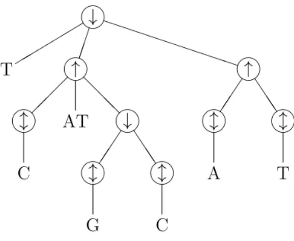
Figure 2.4: The structure tree of the DNA expression from Example 2.12.

has two or more arguments, then its children in the structure tree are arranged from left to right in the same order as the corresponding arguments in the DNA expression. Because every N-word and every proper DNA subexpression of E has exactly one parent operator, we indeed obtain a tree. The leaves of the tree are labelled by the

N-words αoccurring inE, and the internal nodes by the operators. The node labelled by the outermost operator of E is the root of the tree. It corresponds to the entire DNA expression. As an example, in Figure 2.4 we have drawn the structure tree of the DNA expression from Example 2.12.

There is a very close relation between the maximal nesting level of a DNA expression and the height of the corresponding structure tree:

Lemma 2.22 Let E be a DNA expression, let l be the maximal nesting level of E, and let t be the structure tree of E. Then the height of t is l+ 1.

As we observed in § 2.5, the maximal nesting level of the DNA expression from Ex-ample 2.12 is 4. Indeed, the height of the corresponding structure tree in Figure 2.4 is 4 + 1 = 5.

Proof: By induction on the number p of operators occurring in E.

• If p = 1, then E is equal to h↑αi, h↓αi or hlαi for an N-word α. By Lemma 2.14(1), the maximal nesting level of E is l = 1. The structure tree t of E consists of a root, labelled by an operator, with one child node, labelled byα. Indeed, the height of t is 2 =l+ 1.

• Letp≥1, and suppose that the claim holds for all DNA expressions containing at mostp operators (induction hypothesis). Now, assume that E contains p+ 1 operators.

Let E1, . . . , Er for some r ≥ 0 be the expression-arguments of E. Because E

contains p+ 1 ≥ 2 operators, we must have r ≥ 1. Each Ej contains at most p

operators. For j = 1, . . . , r, let lj be the maximal nesting level ofEj.

All about A Minimal Normal Form for DNA Expressions

Technical Report 2011-03

July 2011

Universiteit Leiden

Leiden Institute of Advanced Computer Science

All about a Minimal Normal Form

for DNA Expressions

Rudy van Vliet

Leiden Institute of Advanced Computer Science

Leiden University

Technical Report 2011-03

July 2011

Universiteit Leiden

Leiden Institute of Advanced Computer Science

All about a Minimal Normal Form

for DNA Expressions

Rudy van Vliet

Leiden Institute of Advanced Computer Science

Leiden University

Contents

Preface

Chapter 1

Introduction

Chapter 2

Terminology and Notation

2.1

Strings,

N

-words, trees, grammars and

com-plexity

2.2

Formal DNA molecules

2.3

Properties, relations and functions of formal

DNA molecules

2.4

Operators and DNA expressions

↑

↑

↓

l

2.5

Nesting level of the brackets

2.6

The functions

L

and

R

for arguments of DNA

expressions

2.7

A context-free grammar for

D

2.8

The structure tree of a DNA expression

_{-words, trees, grammars and}