Tony Lindeberg∗
Computational Vision and Active Perception Laboratory (CVAP) Department of Numerical Analysis and Computing Science
KTH (Royal Institute of Technology) S-100 44 Stockholm, Sweden. http://www.nada.kth.se/˜tony
Email: [email protected]
Technical report ISRN KTH/NA/P–96/18–SE, May 1996, Revised August 1998. Int. J. of Computer Vision, vol 30, number 2, 1998. (In press).
Abstract
The fact that objects in the world appear in different ways depending on the scale of observation has important implications if one aims at describing them. It shows that the notion ofscale is of utmost importance when processing unknown measurement data by automatic methods. In their seminal works, Witkin (1983) and Koenderink (1984) proposed to approach this problem byrepresentingimage structures at different scales in a so-called scale-space representation. Traditional scale-space theory building on this work, however, does not address the problem of how toselect local appropriate scales for further analysis.
This article proposes a systematic methodology for dealing with this problem. A framework is proposed forgenerating hypotheses about interesting scale levels in image data, based on a general principle stating thatlocal extrema over scales of different combinations of γ-normalized derivatives are likely candidates to correspond to interesting structures. Specifically, it is shown how this idea can be used as a major mechanism in algorithms for automatic scale selection, which adapt the local scales of processing to the local image structure.
Support for the proposed approach is given in terms of a general theoretical investigation of the behaviour of the scale selection method under rescalings of the input pattern and by experiments on real-world and synthetic data. Support is also given by a detailed analysis of how different types of feature detectors perform when integrated with a scale selection mechanism and then applied to characteristic model patterns. Specifically, it is described in detail how the pro-posed methodology applies to the problems of blob detection, junction detection, edge detection, ridge detection and local frequency estimation.
In many computer vision applications, the poor performance of the low-level vision modules constitutes a major bottle-neck. It will be argued that the inclu-sion of mechanisms for automatic scale selection is essential if we are to construct vision systems to analyse complex unknown environments.
Keywords:scale, scale-space, scale selection, normalized derivative, feature detec-tion, blob detecdetec-tion, corner detecdetec-tion, frequency estimadetec-tion, Gaussian derivative, scale-space, multi-scale representation, computer vision
∗
This work was partially performed under the BRA project INSIGHT and the ESPRIT-NSF collaboration DIFFUSION. The support from the Swedish Research Council for Engineering Sciences, TFR, is gratefully acknowledged. The three-dimensional illustrations in figure 5 and fig-ure 11 have been generated with the kind assistance of Pascal Grostabussiat.
Contents
1 Introduction 1
1.1 Outline of the presentation . . . 2
2 Scale-space representation: Review 3 3 Normalized derivatives and intuitive idea for scale selection 3 4 Proposed methodology for scale selection 5 4.1 General scaling property of local maxima over scales . . . 6
4.2 The scale selection mechanism in practice . . . 8
4.3 Experiments: Scale-space signatures from real data . . . 9
4.4 Simultaneous detection of interesting points and scales . . . 9
5 Blob detection with automatic scale selection 11 5.1 Analysis of scale-space maxima for idealized model patterns . . . 11
5.2 Comparisons with fixed-scale blob detection . . . 14
5.3 Applications of blob detection with automatic scale selection . . . 15
6 Junction detection with automatic scale selection 15 6.1 Selection of detection scales from normalized scale-space maxima . . . 16
6.2 Analysis of scale-space maxima for diffuse junction models . . . 18
6.3 Experiments: Scale-space signatures in junction detection . . . 19
7 Feature localization with automatic scale selection 21 7.1 Corner localization by local consistency . . . 21
7.2 Automatic selection of localization scales . . . 23
7.3 Experiments: Choice of localization scale . . . 25
7.4 Composed scheme for junction detection and localization . . . 27
7.5 Further experiments . . . 28
7.6 Applications of corner detection with automatic scale selection . . . . 32
7.7 Extensions of the junction detection method . . . 32
7.8 Extensions to edge detection . . . 33
8 Dense frequency estimation 34 9 Analysis and interpretation of normalized derivatives 38 9.1 Interpretation ofγ-normalized derivatives in terms of Lp-norms . . . . 38
9.2 Interpretation in terms of self-similar Fourier spectrum . . . 38
9.3 Relations to previous work . . . 40
10 Summary and discussion 40 10.1 Technical contributions . . . 41
A Appendix 42 A.1 Necessity of the form of the γ-parameterized derivative operator . . . 42
A.2 Lp-normalization interpretation of γ-normalized derivatives . . . 44
A.3 Normalized derivative responses to self-similar power spectra . . . 44
1 Introduction
One of the very fundamental problems that arises when analysing real-world mea-surement data originates from the fact that objects in the world may appear in different ways depending upon the scale of observation. This fact is well-known in physics, where phenomena are modelled at several levels of scale, ranging from parti-cle physics and quantum mechanics at fine scales, through thermodynamics and solid mechanics dealing with every-day phenomena, to astronomy and relativity theory at scales much larger than those we are usually dealing with. Notably, the type of phys-ical description that is obtained may be strongly dependent on the scale at which the world is modelled, and this is in clear contrast to certain idealized mathematical entities, such as “point” or “line”, which are independent of the scale of observation. In certain controlled situations, appropriate scales for analysis may be known a priori. For example, a desirable property of a good physicist is his intuitive ability to select appropriate scales to model a given situation. Under other circumstances, however, it may not be obvious at all to determine in advance what are the proper scales. One such example is a vision system with the task of analysing unknown scenes. Besides the inherent multi-scale properties of real world objects (which, in general, are unknown), such a system has to face the problems that the perspective mapping gives rise to size variations, that noise is introduced in the image formation process, and that the available data are two-dimensional data sets reflecting only indirect properties of a three-dimensional world. To be able to cope with these problems, an image representation that explicitly incorporates the notion of scale is a crucially important tool whenever we attempt to interpret sensory data, such as images, by automatic methods.
In computer vision and image processing, these insights have lead to the con-struction of multi-scale representations of image data, obtained by embedding any given signal into a one-parameter family of derived signals (Burt 1981; Crowley 1981; Witkin 1983; Koenderink 1984; Yuille and Poggio 1986; Floracket al.1992; Lin-deberg 1994d; Haar Romeny 1994). This family should be parameterized by a scale parameter and be generated in such a way that fine-scale structures are successively suppressed when the scale parameter is increased. A main intention behind this con-struction is to obtain a separation of the image structures in the original image, such that fine scale image structures only exist at the finest scales in the multi-scale representation. Thereby, the task of operating on the image data will be simplified, provided that the operations are performed at sufficiently coarse scales where unnec-essary and irrelevant fine-scale structures have been suppressed. Empirically, this idea has proved to be extremely useful, and multi-scale representations such as pyramids, scale-space representation and non-linear diffusion methods are commonly used as preprocessing steps to a large number of early visual operations, including feature detection, stereo matching, optic flow, and the computation of shape cues.
A multi-scale representation by itself, however, contains no explicit information about what image structures should be regarded as significant or what scales are ap-propriate for treating those. Hence, unless early judgements can be made about what image structures should be regarded as important, we obtain a substantial expansion of the amount of data to be interpreted by later stage processes. In most previous works, this problem has been handled by formulating algorithms which rely on the information present in the data at a small set of manually chosen scales (or even a single scale). Alternatively, coarse-to-fine algorithms have been expressed, which start at a given coarse scale and propagate down to a given finer scale. Determining such
scales in advance, however, leads to the introduction of free parameters. If one aims at autonomous algorithms which are to operate in a complex environment without need for external parameter tuning, we therefore argue that it is essential to complement traditional multi-scale processing by explicit mechanisms for scale selection. Notably, image descriptors can be highly unstable if computed at inappropriately chosen scales, whereas a proper tuning of the scale parameter can improve the quality of an image descriptor substantially. As will be demonstrated later, local scale information can also constitute an important to in its own right.
Early work addressing this problem was presented in (Lindeberg 1991, 1993a) for blob-like image structures. The basic idea was to study the behaviour of image structures over scales, and to measure the saliency of image structures from the stability properties and the lifetime of these structures in scale-space. Scale levels were selected from the scales at which a measure of blob strength assumed local maxima over scales and significant image structures from the stability of the blob structures in scale-space. Experimentally, it was shown that this approach could be used for extracting regions of interest with associated scale levels, which in turn could serve as to guide various early visual processes.
The subject of this article is to address the problem of automatic scale selection in a more general setting, for wider classes of image descriptors. We shall be con-cerned with the problem of extracting image features and computing filter-like image descriptors, and present a scale selection principle for image descriptors which can be expressed in terms of Gaussian derivative filters. The general idea for scale selection that will be proposed is to study theevolution properties over scalesof normalized dif-ferential descriptors. Specifically, it will be suggested thatlocal extrema over scales of suchnormalized differential entities, which arise in this way, are likely to correspond to interesting image structures. By theoretical considerations and experiments it will be shown that this approach gives rise to intuitively reasonably results in different situations and that it provides a unified framework for scale selection for detecting image features such as blobs, corners, edges and ridges.
1.1 Outline of the presentation
The presentation is organized as follows: Section 2 reviews the main concepts from scale-space theory we build upon. Section 3 introduces the notion of normalized derivatives and illustrates how maxima over scales of normalized Gaussian deriva-tives reflect the frequency content in sine wave patterns. This material serves as a preparation for section 4, which presents the proposed scale selection methodology and shows how it applies generally to a large class of differential descriptors. Sec-tion 4 also proposes a general extension of the common idea of defining features as zero-crossings of spatial differential descriptors. If a scale selection mechanism is inte-grated into such a feature detector, this corresponds to adding another zero-crossing requirement over the scale dimension in the differential feature definition.
Then, section 5 and section 6 show in detail how these ideas can be used for for-mulating blob detectors and corner detectors with automatic scale selection. Section 8 shows an example of how this approach applies to the computation of dense feature maps. Section 9 describes different ways of interpreting the normalized derivative con-cept. Finally, section 10 summarizes the main results and ideas of the approach. In a complementary paper (Lindeberg 1996a) it is developed in detail how this approach applies to edge detection and ridge detection.
Earlier presentations of different parts of this material have appeared elsewhere (Lindeberg 1993b, 1994a, 1994d, 1996b) as well as applications of the general ideas to
various problem domains (Lindeberg and G˚arding 1993, 1997; G˚arding and Lindeberg 1996; Lindeberg and Li 1995, 1997; Bretzner and Lindeberg 1998, 1997; Almansa and Lindeberg 1996; Wiltschi et al.1997; Lindeberg 1997). The subject of this paper is to present a coherent description of the proposed scale selection methodology in journal form, including the developments and refinements that have been performed since the earliest presented manuscripts.
2 Scale-space representation: Review
Given any continuous signals f: RD → R, the (linear) scale-space representation
L:RD×R+→Rof f is defined as the solution to the diffusion equation
∂tL= 1 2∇
2L= 1
2 D X
i=1
∂xixiL (1)
with initial condition L(·; 0) = f(·). Equivalently, this family can be defined by convolution with Gaussian kernels of various widtht
L(·; t) =g(·; t)∗f(·), (2) whereg: RD ×R+→Ris given by
g(x; t) = 1 (2πt)N/2e
−(x21+...+x2D)/(2t), (3)
and x = (x1, ..., xD)T. There are several mathematical results (Koenderink 1984; Babaud et al. 1986; Yuille and Poggio 1986; Lindeberg 1990, 1994d, 1994b; Koen-derink and van Doorn 1990, 1992; Florack et al. 1992; Florack 1993; Florack et al. 1994; Pauwels et al.1995) stating that within the class of linear transformations the Gaussian kernel is the unique kernel for generating a scale-space. The conditions that specify the uniqueness are essentially linearity and shift invariance combined with different ways of formalizing the notion that new structures should not be created in the transformation from a finer to a coarser scale.
Interestingly, the results from these theoretical considerations are in qualitative agreement with the results of biological evolution. Neurophysiological studies by (Young 1985, 1987) have shown that there are receptive fields in the mammalian retina and visual cortex, whose measured response profiles can be well modelled by Gaussian derivatives up to order four. In these respects, the scale-space representa-tion with its associated Gaussian derivative operators (whereα denotes the order of differentiation)
Lxα(·; t) = (∂xαL)(·,·; t) =∂xα(g∗f) = (∂xαg)∗f =g∗(∂xαf), (4)
can be seen as a canonical idealized model of a visual front-end. It is for this multi-scale representation concept we will develop the multi-scale selection methodology.
3 Normalized derivatives and intuitive idea for scale selection A well-known property of the scale-space representation is that the amplitude of spatial derivatives
Lxα(·; t) =∂xαL(·; t) =∂
in generaldecrease with scale, i.e., if a signal is subject to scale-space smoothing, then the numerical values of spatial derivatives computed from the smoothed data can be expected to decrease. This is a direct consequence of the non-enhancement property of local extrema, which states that the value at a local maximum cannot increase, and the value at a local minimum cannot decrease. In practice, it means that the amplitude of the variations in a signal will always decrease with scale.
As a simple example of this, consider a sinusoidal input signal1 of some given frequencyω0; for simplicity in one dimension,
f(x) = sinω0x. (6)
It is straightforward to show that the solution of the diffusion equation is given by
L(x; t) =e−ω20t/2sinω0x. (7) Hence, the amplitude of the scale-space representation,Lmax, as well as the amplitude of the mth order smoothed derivative, Lxm,max, decrease exponentially with scale
Lmax(t) =e−ω02t/2, Lxm,max(t) =ωm0 e−ω
2
0t/2. (8)
Let us next introduce aγ-normalized derivative operator defined by
∂ξ,γ−norm =tγ/2∂x, (9) which corresponds to the change of variables
ξ= x
tγ/2. (10)
In the special case when γ = 1, these ξ-coordinates and their associated normalized derivative operator are dimensionless. The property of perfect scale invariance has been used by (Florack et al. 1992) as a main requirement in an axiomatic scale-space formulation (see also (Pauwels et al.1995; Lindeberg 1994b)). As we shall see later, however, values ofγ <1 will be highly useful when formulating scale selection mechanisms for edge detection and ridge detection.
For the sinusoidal signal, the amplitude of anmth order normalized derivative as function of scale is then given by
Lξm,max(t) =tmγ/2ω0me−ω20t/2, (11)
i.e., it first increases and then decreases. Moreover, it assumes a unique maximum at
tmax,Lξm =γ m/ω
2
0. If we define a scale parameterσ of dimension length byσ =
√
t
and introduce the wavelength λ0 of the signal by λ0 = 2π/ω0, we can see that the
scale at which the amplitude of the γ-normalized derivative assumes its maximum over scales isproportional to the wavelength, λ0, of the signal:
σmax,Lξm =
√γ m
2π λ0. (12)
The maximum value over scales is
Lξm,max(tmax,Lξm) =
(γm)γm/2
eγm/2 ω
(1−γ)m
0 . (13)
1An analysis of scale-space like responses to sine waves corresponding to the case whenγ= 1 in this section has also been performed in wavelet analysis by (Mallat and Hwang 1992); see section 9.3.
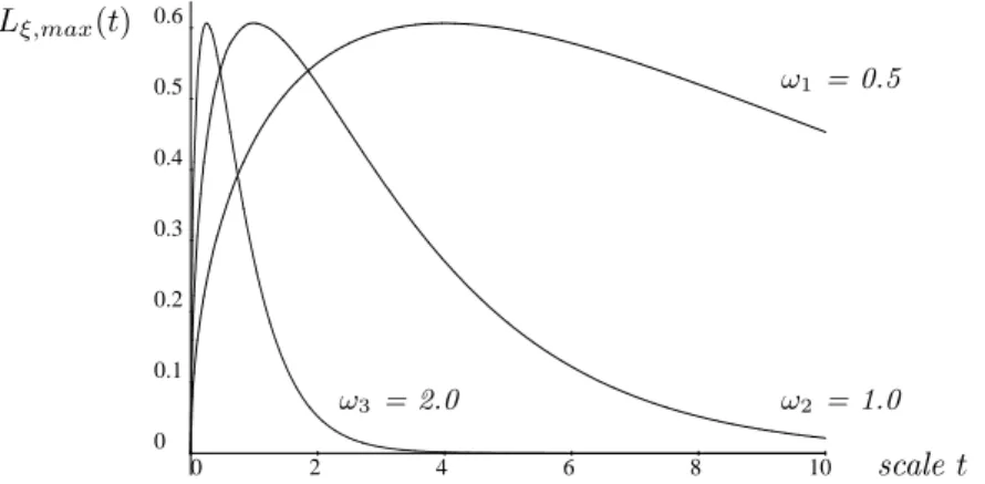
In the case when γ = 1, this maximum value is independent of the frequency of the signal (see figure 1), and the situation is highly symmetric, i.e., given any scale t0,
the maximally amplified frequency is given by ωmax = pm/t0, and for any ω0 the
scale with maximum amplification is tmax = m/ω20. In other words, for normalized
derivatives with γ = 1 it holds that sinusoidal signals are treated in a similar (scale invariant) way independent of their frequency (see figure 1). The situation is a bit different whenγ 6= 1. We shall return to this subject in section 4.1.
4 Proposed methodology for scale selection
The example above shows that the scale at which a normalized derivative assumes its maximum over scales is for a sinusoidal signal proportional to the wavelength of the signal. In this respect, maxima over scales of normalized derivatives reflect the scales over which spatial variations take place in the signal.
Yhis operation corresponds to an interesting computational structure, since it constitutes a way of estimating length based on local measurements performed at only a single spatial point in the scale-space representation, and without explicitly laying out a ruler. Moreover, compared to a local windowed Fourier transform there is no need for making any explicit settings of window size for computing the Fourier transform. Instead, the propagation of length information over space is performed via the diffusion equation, and the decisions about the contents in the data are made by studying the output of derivative operators as the diffusion process evolves.
Alternatively, we can view such a measurement procedure as a pattern matcher, which matches Gaussian derivative kernels of different size to the given image pattern, based on a specific normalization of the primitive templates. By using the proposedγ -normalized derivative concept for normalization, we obtain one-to-one correspondence between the matching response of the Gaussian derivative kernels and the wavelength of the signal. Selecting the scale at which the maximum over scale is assumed cor-responds to selecting the pattern (or the scale) for which the operator response is strongest.
This property is, however, not restricted to sine wave patterns or to image mea-surements in terms of linear derivative operators of a certain order. Contrary, it applies to a large class of image descriptors which can be formulated as multi-scale differen-tial invariants expressed in terms of Gaussian derivatives (this notion will be made more precise next). A main message of this article is that this property can be used as
0 2 4 6 8 10
0 0.1 0.2 0.3 0.4 0.5 0.6
scale t Lξ,max(t)
ω3 = 2.0 ω2 = 1.0
ω1 = 0.5
Figure 1:The amplitude of first order normalized derivatives as function of scale for sinu-soidal input signals of different frequencies (ω1= 0.5,ω2= 1.0 andω3= 2.0).
a major mechanism in algorithms for automatic scale selection, which automatically adapt the local scales of processing to image data. Let us hence generalize the above-mentioned observation to more complex signals and state the following principle for scale selection, to be applied in situations when no other information is available. In its most general form, it can be expressed as follows:
Principle for scale selection:
In the absence of other evidence, assume that a scale level, at which some (possibly non-linear) combination of normalized derivatives assumes a local maximum over scales, can be treated as reflecting a characteristic length of a corresponding structure in the data.
This principle is closely related to although not equivalent to the method for scale selection in previously proposed in (Lindeberg 1991, 1993a), where interesting scale levels were determined from maxima over scales of a normalized blob measure. It can be theoretically justified under a number of different assumptions and for a number of specific brightness models (see next). Its general usefulness, however, must be verified empirically, and with respect to the type of problem it is to be applied to.
4.1 General scaling property of local maxima over scales
A basic justification for the abovementioned arguments can be obtained from the fact that for a large class of (possibly non-linear) combinations of normalized derivatives it holds that maxima over scales have a nice behaviour under rescalings of the intensity pattern. If the input image is rescaled by a constant scaling factors, then the scale at which the maximum is assumed will be multiplied by the same factor (if measured in units ofσ =√t). This is a fundamental requirement on a scale selection mechanism, since it guarantees that the image operations will commute with size variations. Transformation properties under rescalings: To give a formal characterization of this scaling property, consider two signalsf and f0 related by
f(x) =f0(sx), (14) and define the scale-space representations off and f0 in the two domains by
L(·; t) =g(·; t)∗f, (15)
L0(·; t0) =g(·; t0)∗f0, (16) where the spatial variables and the scale parameters are transformed according to
x0 =sx, (17)
t0 =s2t. (18)
Then,L andL0 are related by
L(x; t) =L0(x0; t0), (19) and the mth order spatial derivatives satisfy
∂xmL(x; t) =sm∂x0mL0(x0; t0). (20)
Finally, for γ-normalized derivatives defined in the two domains by
∂ξ =tγ/2∂x, (21)
we have that
∂ξmL(x; t) =sm(1−γ)∂ξ0mL0(x0; t0). (23)
Perfect scale invariance when γ = 1: From this relation it can be seen that, when
γ = 1 the normalized derivative concept leads to perfect scale invariance. The nor-malized derivatives are equal in the two domains, provided that the scale parameters and the spatial positions are matched according to (17) and (18). More specifically, local maxima over scales are always assumed at corresponding positions, and this scaling property holds for any differential expression defined from the localN-jet. Sufficient scale invariance when γ 6= 1: The case when γ 6= 1 leads to a different type of structure, since we cannot preserve a scaling property for arbitrary combi-nations of normalized derivatives. Let us hence restrict the analysis to polynomial differential invariants which are homogeneous in the sense that the sum of the orders of differentiation is the same for each term in the polynomial. To express this no-tion compactly, introduce multi-index notano-tion for derivatives byLxα =L
xα11xα22...xαDD where x= (x1, x2, . . . xD),α = (α1, α2, . . . αD) and |α|=α1+α2+· · ·+αD. Then, consider a homogeneous polynomial differential invariant DLof the form
DL=
I X
i=1
ci J Y j=1
Lxαij, (24)
where the sum of the orders of differentiation in a certain term J
X j=1
|αij|=M (25)
does not depend on the indexiof that term. For a differential expression of this form, the corresponding normalized differential expression in each domain is given by
Dγ−normL=tM γ/2DL, (26)
D0
γ−normL0 =t0M γ/
2D0
L0. (27)
From (23) it follows that these normalized differential expressions are related by
Dγ−normL=sM(1−γ)Dγ0−normL0. (28)
Clearly, by γ-normalization with γ = 1, the magnitude of the derivative is not scale invariant. Local maxima over scales will, however, still be preserved, since
∂t(Dγ−normL) = 0 ⇔ ∂t0 Dγ0−normL0= 0 (29) and the type of critical points are preserved under this transformation. Hence, even when γ 6= 1, we can achieve sufficient scale invariance to support the proposed scale selection methodology.
Scale compensated magnitude measures when γ 6= 1: When basing a scale selection methodology onγ 6= 1, there is, however, a minor complication which needs attention. When performing feature detection in practice, it is natural to associate a measure of feature strength with each detected feature. Specifically, the magnitude of the response at the local maximum over scales constitutes a natural entity to include in
such a measure. From the the transformation property (23), it is, however, apparent that this magnitude measure will be strongly dependent on the scale at which the maximum over scales is assumed. Hence, the magnitude measure will depend on the feature size. In view of the scale invariant magnitude measure obtained usingγ = 1, it is, however, straightforward to correct for this phenomenon by multiplying the response by a correction factor and to define a compensated magnitude measure by
Mγ−normL=tM(1−γ)/2Dγ−normL. (30)
Then, the magnitude measures in the two domains will satisfy
Mγ−normL(x; t) =M0γ−normL0(x0; t0). (31) Necessity of theγ-normalization: More generally, one may ask what choices of nor-malization factors are possible, provided that we would like to state this scaling property as a fundamental constraint on a scale selection mechanism based on local maxima over scales of normalized differential entities. Then, in fact, it can be shown that theγ-normalized derivative concept according to (9) arises by necessity.
In other words, the γ-normalized derivative concept comprises the most general class of normalization factors for which detection of local maxima over scales com-mutes with rescalings of the input pattern. A more precise formulation of this state-ment as well as the details of the necessity proof can be found in appendix A.1. Summary: Scale selection properties: To conclude, this analysis shows that if a γ -normalized homogeneous differential expression assumes a maximum over scales at (x0;t0) in the scale-space representation of f, then there will be a corresponding
maximum over scales in the scale-space representation off0 at (s x0;s2t0). Moreover,
although the magnitude of a normalized derivative at a local maximum over scales is not scale invariant unlessγ = 1, it is possible to compensate for this phenomenon and to define scale invariant magnitude descriptors also whenγ 6= 1.
4.2 The scale selection mechanism in practice
So far we have proposed a general methodology for scale selection by detecting local maxima in feature responses over scales. Whereas this approach constitutes an exten-sion of the traditional way in which spatial features are detected from spatial maxima of feature responses, there is a fundamental difference. Since the image operators at different scales by necessity have to be of different size, the problem of normalizing the filter responses is of crucial importance. In section 4.1, we analysed this prob-lem in detail and investigated the feasibility of capturing image structures under size variations. Specifically, we characterized general classes of differential invariants as well as normalization approaches, which allow for scale selection within the proposed computational structure. A fundamental problem that remains to be solved in this context concerns what differential expressions to use. Is any differential invariant fea-sible? Here, we shall not attempt to answer this question. Let us instead contend that the differential expression should at least be determined so as to capture the types of image structures under consideration.
The general approach to scale selection that will be proposed is to use these maximal responses over scales in the stage of detecting image features,i.e., when es-tablishing the existence of different types of image structures. Basically, the scale at which a maximum over scales is attained will be assumed to give information about how large a feature is, in analogy with the common approach of taking the spatial
position at which the maximum operator response is assumed as an estimate of the spatial location of a feature. In certain situations, and as we shall see more specific examples of later, this implies that image features may be detected at quite coarse scales, and the localization properties may not be the best. Therefore, we propose to complement this framework by a second processing stage, in which more refined pro-cessing is invoked for computing more accurate localization estimates. In this respect, the suggested framework naturally gives rise to two-stage algorithms, with feature detection at coarse scales followed by feature localization at finer scales. Whereas coarse-to-fine approaches are common practice in several computer vision problems, a notable aspect of this approach will be that we include explicit mechanisms for automatic selection of all scale parameters.
In the following, we shall shift attention to the application of the abovementioned general ideas to specific problems. A series of theoretical and experimental results will be presented showing how the proposed approach applies to different types of feature detectors expressed as polynomial combinations of Gaussian derivatives.
4.3 Experiments: Scale-space signatures from real data
Figure 2 shows the variations over scales of two simple differential expressions formu-lated in terms of normalized derivatives. It shows the result of computing the trace and the determinant of the normalized Hessian matrix by (with γ = 1)
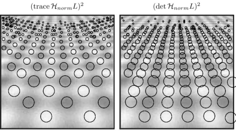
traceHnormL=tγ∇2L=tγ(Lxx+Lyy), (32) detHnormL=t2γ(LxxLyy−L2xy), (33) for two details in an image of a field of sunflowers. (To avoid the sensitivity to sign of these entities, and hence the polarity of the signal, traceHnormLand detHnormLhave been squared before presentation.) These graphs are called thescale-space signatures of (traceHnormL)2 and (detHnormL)2, respectively.
As can be seen, the maximum over scales in the top row of figure 2 is assumed at a finer scale than in the bottom row. A more detailed examination the ratio between the scale values2 where the graphs attain their maxima over scales shows that when the scale parameter is measured in dimension length this scale ratio is roughly equal to the ratio of the diameters of the sunflowers in the centers of the two images, respectively. This example illustrates that results in agreement with the proposed scale selection principle can be obtained also for real-world data (and for signals having a much richer frequency content than a single sine wave).
The reason why these particular differential expressions have been selected here is because they constitute differential entities useful for blob detection; seee.g.(Marr 1982; Voorhees and Poggio 1987; Blostein and Ahuja 1989). Before we turn to the problem of expressing an integrated blob detector with automatic scale selection, however, let us describe a further extension of the general scale selection idea. 4.4 Simultaneous detection of interesting points and scales
In figure 2, the signatures of the normalized differential entities were computed at the central point in each image. These points were deliberately chosen to coincide 2 In the graphs in figure 2 the scale parameter (on the horizontal axis) is measured in terms ofeffective scale,τ. For continuous signals, this parameter is essentially the logarithm of the scale parameter τ =C1logt+C2 for some C1,C2 >0. To avoid the singularity at zero scale, however, all experiments are based on an effective scale concept especially developed for discrete signals and defined such thatτ∼logtat coarse scales andτ∼tat fine scales see (Lindeberg 1994d).
(traceHnormL)2 (detHnormL)2
0 1 2 3 4 5 6 7
0 200 400 600 800 1000 1200 1400
0 1 2 3 4 5 6 7
0 20000 40000 60000 80000 100000
0 1 2 3 4 5 6 7
0 500 1000 1500 2000
0 1 2 3 4 5 6 7
0 50000 100000 150000 200000
Figure 2: Scale-space signatures of the trace and the determinant of the normalized Hes-sian matrix computed for two details of a sunflower image; (left) grey-level image, (middle) signature of (traceHnormL)2, (right) signature of (detHnormL)2. (The signature have been computed at the central point in each image. The horizontal axis shows effective scale (essen-tially the logarithm of the scale parameter), whereas the scaling of the vertical axis is linear in the normalized operator response.)
with the centers of the sunflowers, where the blob response can be expected to be maximal under spatial perturbations. In a real-world vision situation, however, we cannot assume such points to be known a priori. Moreover, we can expect that the spatial maximum of the operator response is assumed at different positions at different scales. This is one example of the well-known fact that scale-space smoothing leads to shape distortions.
Therefore, a more general approach to scale selection from local extrema in the scale-space signature is by accumulating the signature of any normalized differential entityDnormLalong the pathr:R+→RNthat a local extremum inDnormLdescribes across scales. The mathematical framework for describing such paths is described in (Lindeberg 1994d). Formally, an extremum path of a differential entity DnormL is defined (from the implicit function theorem) as a set of points (r(t); t) ∈RN ×R+
in scale-space such that for any t ∈ R+ the point r(t) is a local extremum of the
mappingx7→(DnormL)(x; t),
{(x; t)∈RN×R+}={(r(t); t)∈RN ×R+: (∇(DnormL))(r(t); t) = 0}.
At the point at which an extremum in the signature is assumed, the derivative along the scale direction is zero as well. Hence, it is natural to define a normalized scale-space extremum of a differential entity DnormL as a point (x0; t0) ∈ RN ×R+ in
coordinates and the scale parameter.3 In terms of derivatives, such points satisfy
(∇(DnormL))(x0; t0) = 0,
(∂t(DnormL))(x0; t0) = 0.
(34) These normalized scale-space extrema constitute natural generalizations of extrema with respect to the spatial coordinates, and can serve as natural interest points for feature detectors formulated in terms of spatial maxima of differential operators, such as blob detectors, junction detectors, symmetry detectors, etc. Specific examples of this idea will be worked out in more detail in the following sections.4
Referring to the invariance properties of local maxima over scales under rescalings of the input signal, we can observe that they transfer trivially to scale-space maxima. Hence, if a normalized scale-space maximum is assumed at (x0; t0) in the scale-space
representation of a signal f, then in a rescaled signal f0 defined by f0(sx) = f(x), a corresponding scale-space maximum is assumed at (sx0; s2t0) in the scale-space
representation of f0.
5 Blob detection with automatic scale selection
Figure 3 shows the result of detecting normalized scale-space extrema of the normal-ized Laplacian in an image of a sunflower field. Every scale-space maximum has been graphically illustrated by a circle centered at the point at which the spatial maxi-mum is assumed, and with the size determined such that the radius (measured in pixel units) is proportional to the scale at which the maximum is assumed (measured in dimension length). To reduce the number of blobs, a threshold on the maximum normalized response has been selected such that the 250 blobs having the maximum normalized responses according to (30) remain.
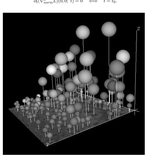
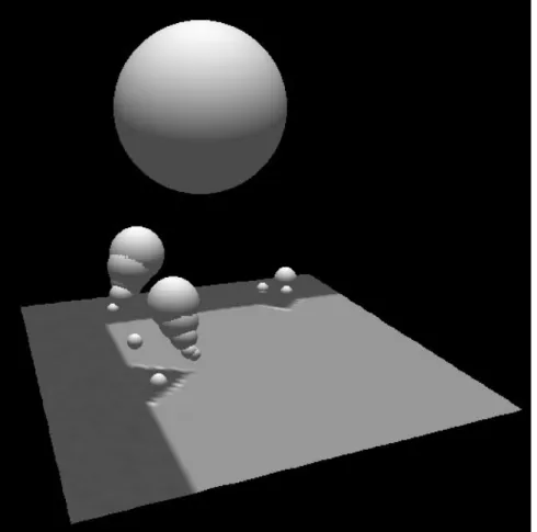
The bottom row shows the result of superimposing these circles onto a bright copy of the original image, as well as corresponding results for the normalized scale-space extrema of the square of the determinant of the Hessian matrix. Corresponding experiments for a synthetic pattern (analysed in section 5.1) are given in figure 4. Observe how these conceptually very simple differential geometric descriptors give a very reasonable description of the blob-like structures in the image (in particular concerning the blob size) considering how little information is used in the processing. Figure 5 shows a three-dimensional illustration of the multi-scale blob descrip-tors computed from the sunflower image. Here, each scale-space maximum has been visualized by a sphere centered at the position (x0; t0) in scale-space at which the
maximum was assumed, with the radius proportional to the selected scale, and the brightness increasing with the significance of the blob. Observe how the size variations in the image data are reflected in the spatial variations of the image descriptors. 5.1 Analysis of scale-space maxima for idealized model patterns
Whereas the theoretical analysis in section 4.1 applies generally to large classes of differential invariants and input signals, one may ask how the scale selection method for blob detection performs in specific situations. In this section, we shall study two 3When detecting scale-space maxima in practice, there is, of course, no need to explicitly track the extrema along the extremum path in scale-space. It is sufficient to detect three-dimensional maxima over space and scale (as described in more detail in section A.4.3).
4Further extensions of this idea are also explored in (Lindeberg 1996a), where differential defini-tions of edges and ridges are expressed in such a way that scale selection constitutes an integrated part of the feature definition.
original image scale-space maxima of(∇2normL)2
(traceHnormL)2 (detHnormL)2
Figure 3:Normalized scale-space maxima computed from an image of a sunflower field: (top left): Original image. (top right): Circles representing the 250 normalized scale-space maxima of (traceHnormL)2having the strongest normalized response. (bottom left): Circles represent-ing scale-space maxima of (traceHnormL)2 superimposed onto a bright copy of the original image. (bottom right): Corresponding results for scale-space maxima of (detHnormL)2.
(traceHnormL)2 (detHnormL)2
Figure 4:The 250 most significant normalized scale-space extrema detected from the per-spective projection of a sine wave of the form (with 10% added Gaussian noise).
model patterns for which a closed-form solution of diffusion equation can be calculated and a complete analytical study hence is feasible.
Example 1. Consider first a non-symmetric Gaussian function
f(x1, x2) =g(x1; t1)g(x2; t2) =
1
√
2πt1
e−x21/2t1 √1 2πt2
e−x22/2t2
as a model of a two-dimensional blob with characteristic lengths√t1and
√
t2along the
coordinate directions. From the semi-group property of the Gaussian kernelg(·; tA)∗
g(·; tB) =g(·; tA+tB) it follows that the scale-space representation Lof f is
L(x1, x2; t) =g(x1; t1+t)g(x2; t2+t). (35)
After a few algebraic manipulations it can be shown that for any t1, t2 >0 there is a
unique maximum over scales in
|(∇2normL)(0,0; t)|= t(t1+t2+ 2t) 2π(t1+t)3/2(t2+t)3/2
. (36)
In the case whent1 =t2=t0, this maximum over scales is given by
∂t(∇2normL)(0,0; t) = 0 ⇐⇒ t=t0. (37)
Figure 5: Three-dimensional view of the 150 strongest scale-space maxima of the square of the normalized Laplacian of the Gaussian computed from the sunflower image. (A dark copy of the original grey-level image is shown in the ground plane, and the vertical dimension represents scale.)
The closed-form solution for the maximum over scales in
|detHnorm(0,0; t)|=
t2
4π2(t
1+t)2(t2+t)2
(38) is simple. It is assumed at
tdetHL=
√
t1t2, (39)
verifying that for both traceHnormL and detHnormL the scale at which the scale-space maximum is assumed reflects a characteristic size of the blob.
Example 2. Another interesting special case to consider is a periodic signal defined as the sum of two perpendicular sine waves,
f(x, y) = sinω1x+ sinω2y (ω1≤ω2). (40)
Its scale-space representation is
L(x, y; t) =e−ω12t/2sinω1x+e−ω22t/2sinω2y, (41) and∇2normLand detHnormL assume their spatial maxima at (π/2, π/2). Setting the derivative ∂t|(∇2
normL)(π2,π2; t)|=∂t(t(ω12e−ω
2
1t/2+ω2
2e−ω
2
2t/2)) to zero gives
ω12(2−ω21t)e−ω21t/2+ω22(2−ω22t)e−ω22t/2= 0. (42) There is a unique solution when the ratio ω2/ω1 is close to one, and three solutions
when the ratio is sufficiently large. Hence, there is a unique maximum over scales whenω2/ω1 is close to one, and two maxima when the ratio is sufficiently large. (The
bifurcation occurs when ω2/ω1 ≈ 2.4.) In the special case when ω1 = ω2 = ω0, the
maximum over scales is assumed at
ttraceHL=
2
ω20. (43)
Similarly, setting ∂t|(detHnormL)(π/2, π/2; t)| = ∂t(t2ω21e−ω
2
1t/2ω22e−ω22t/2) to zero gives that the maximum over scales in detHnormLis assumed at
tdetHL= 4
ω21+ω22. (44)
Hence, for both the Gaussian blob model and the periodic sine waves, these specific results agree with the suggested general scale selection principle. When the scale parameter is measured in units ofσ =√t, the scale levels, at which the maxima over scales are assumed, reflect the characteristic length of the structures in the signal. 5.2 Comparisons with fixed-scale blob detection
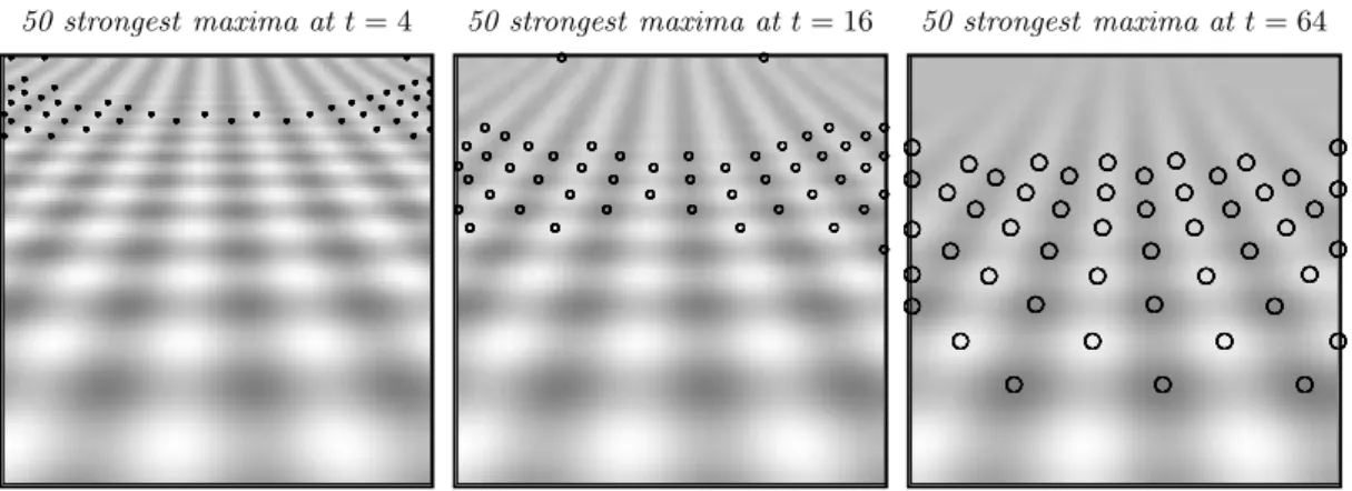
In view of the results presented so far, it is interesting to compare this blob detector with automatic scale selection to a standard multi-scale blob detector operating at a fixed scale. Figure 6 shows the result of computing spatial maxima at different scales in the response of the Laplacian operator from the sine wave pattern in figure 4. At each scale, the 50 strongest responses have been extracted.
As can be seen, small blobs are given the highest relative ranking at fine scales, whereas large blobs are given the highest relative ranking at coarse scales. Hence, a
50 strongest maxima att= 4 50 strongest maxima att= 16 50 strongest maxima att= 64
Figure 6:The 50 strongest spatial responses to the Laplacian operator computed at the scale levels: (a)t= 4.0, (b) t= 16.0, and (c)t= 64.0. Observe how this blob detector leads to a bias towards image structures of a certain size.
blob detector of this type (operating at a single predetermined scale) induces a bias towards image structures of a certain size. On the other hand, if we use the proposed methodology for blob detection based on the detection of scale-space maxima, we obtain a conceptually clean way of handling image structures of all sizes (between the inner scale and the outer scale of the analysis) in a similar manner. (As was shown above, the associated measure of blob strength is strictly scale invariant.)
5.3 Applications of blob detection with automatic scale selection
Following the previously presented arguments, we argue that a scale selection mech-anism is an essential complement to any blob detector aimed at handling large size variations in the image structures. In addition, scale information associated with such adaptively computed image descriptors may serve as an important cue in its own right. In (Bretzner and Lindeberg 1996, 1998) an application to feature tracking is pre-sented, where (i) the scale information constitutes a key component in the criterion for matching image features over time, and (ii) the scale selection mechanism is es-sential for the vision system to be able to capture objects under large size variations over time.
In (Lindeberg and G˚arding 1993; G˚arding and Lindeberg 1996) an extension of this general blob detection idea is presented, where: (i) each scale-space maximum is used for guiding the computation of a regional image texture descriptor (a second moment matrix) as a pre-processing stage to shape-from-texture, (ii) the shape of each blob is represented by an ellipse with its shape determined from the local statistics of image gradient directions, and (iii) the scale information is used as a cue to three-dimensional surface shape when it can be assumed that the texture elements on the surface have the same size.
6 Junction detection with automatic scale selection
A similar approach as was used for blob detection in previous section can be used for detecting corners in grey-level images. In this section, it will be shown how a multi-scale junction detector can be formulated in terms of the scale-space maxima of a normalized differential invariant.
6.1 Selection of detection scales from normalized scale-space maxima
A commonly used entity for junction detection is the curvature of level curves in intensity data multiplied by the gradient magnitude (Kitchen and Rosenfeld 1982; Dreschler and Nagel 1982; Koenderink and Richards 1988; Noble 1988; Deriche and Giraudon 1990; Blom 1992; Florack et al.1992; Lindeberg 1994d). A special choice is to multiply the level curve curvature by the gradient magnitude raised to the power of three. This is the smallest value of the exponent that leads to a polynomial expression
˜
κ=L2vLuu=L2x2Lx1x1−2Lx1Lx2Lx1x2 +L2x1Lx2x2. (45) Moreover, the spatial maxima of this operator are invariant under affine transforma-tions. The corresponding normalized differential expression is obtained by replacing each derivative operator ∂xi by tγ/2∂xi, which gives
˜
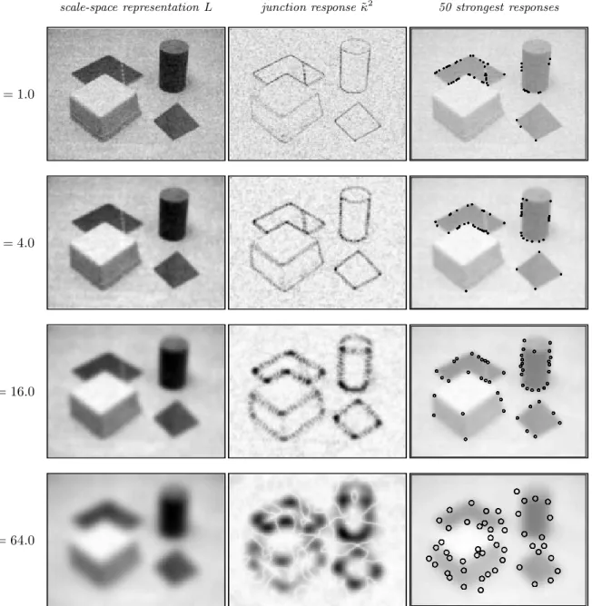
κnorm =t2γ˜κ. (46) Figure 7 shows the results of applying this operator to a grey-level image at a number of different scales. The results are displayed in two ways; (i) in terms of grey-level images showing the scale-space representation L as well as the junction response ˜κ2
computed at each scale, and (ii) in terms of the 50 strongest spatial maxima of ˜κ2, respectively, extracted at the same scale levels. As can be seen, qualitatively different responses are obtained at different scales. At fine scales, the strongest responses are obtained for the sharp corners and for a number of spurious fine-scale perturbations along edges. Then, with increasing values of the scale parameter, the selectivity to junction-like structures increases. In particular, the diffuse (non-sharp) and strongly rounded corners only give rise to strong responses at coarse scales. In summary, this example illustrates the following fundamental aspects of multi-scale corner detection:
• If we are only interested in sharp ideal corners, i.e., corners which can be well approximated by straight lines and for which the intensity contrast across the edge is high and corresponds to a step edge, then it is often sufficient to use a fine scale in the detection stage. The main motivation for using coarser scales on such data is to reduce the number of false positives.
• If we are interested in capturing rounded corners and corners for which the intensity variations across the edges around the junction are slow (diffuse cor-ners), then it is essentially necessary to use a coarse scale if we want to have strong spatial maxima in the response of ˜κ2 at such image structures.
Specifically, this example shows that if noa priori information is available about what can be expected to be in the scene, then a mechanism for automatic scale selection is essential to capture corner structures at different scales.
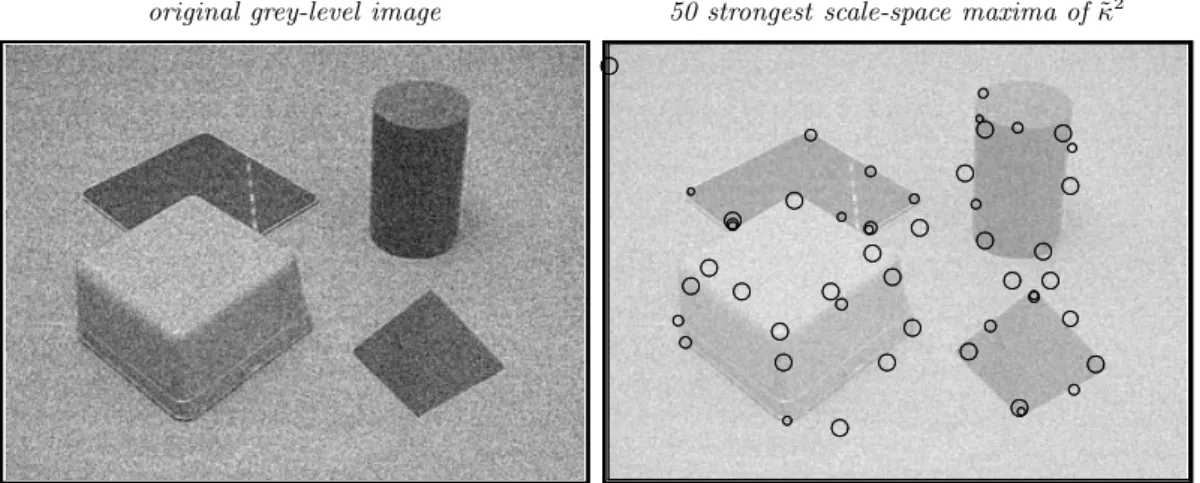
Figure 8 shows the result of including such a scale selection mechanism in the junction detector. It shows the result of detecting the 50 strongest normalized scale-space maxima of ˜κ2norm from the same grey-level image. Each scale-space maximum has been graphically illustrated by a circle centered at the point at which the maximum is assumed, and with the size determined such that the radius is proportional to the scale at which the maximum over scales was assumed (measured in dimension length). To reduce the number of junction candidates, the scale-space maxima have been sorted with respect to a saliency measure. This measure has been determined as the magnitude of the normalized response according to (30) multiplied by the scale parameter measured in dimension area, so as to approximate the area of the spatial
scale-space representation L junction response ˜κ2 50 strongest responses
t= 1.0
t= 4.0
t= 16.0
t= 64.0
Figure 7: Junction responses at different scales computed from a noisy image containing a number of ideal sharp corners as well as rounded and diffuse corners. As can be seen, different types of junction structures give rise to different types of responses at different scales. Notably, certain diffuse junction structures fail to give rise to dominant responses at the finest levels of scale. (Image size: 320*240 pixels.)
original grey-level image 50 strongest scale-space maxima of˜κ2
Figure 8:Junction detection with automatic scale selection: The result of computing the 50 most significant normalized scale-space extrema of ˜κ2normfrom a grey-level image containing sharp straight edges as well as diffuse and rounded edges (withγ= 1). Compare with figure 7 and observe how corner structures at different scales are captured by this operation.
support region of each scale-space maximum. Finally, the 50 most significant blobs according to this ranking have been displayed.
Of course, thresholding on the magnitude of the operator response constitutes a coarse selective mechanism for feature detection. Nevertheless, note that this opera-tion gives rise to a set of juncopera-tion candidates with reasonable interpretaopera-tions in the scene. Moreover, observe that the circles representing the scale-space extrema con-stitute natural regions of interest around the candidate junctions. In particular, the selected scales reflect the diffuseness and the spatial extent of the corners, such that coarser scales are, in general, selected for the diffuse corners than for sharp ones. 6.2 Analysis of scale-space maxima for diffuse junction models
To obtain an intuitive understanding of the qualitative behaviour of the scale selection method in this case, let us analyse a simple junction model for which a closed-form analysis can be carried out without too much effort.
Diffuse step junction. Consider
f(x1, x2) = Φ(x1; t0) Φ(x2; t0) (47)
as a simple model of adiffuseL-junction, where Φ(·; t0) describes adiffuse step edge
Φ(xi; t0) =
Z xi x0=−∞
g(x0; t0)dx0 (48)
with diffuseness t0. From the semi-group property of the Gaussian kernel it follows
that the scale-space representationL of f is
L(x1, x2; t) = Φ(x1; t0+t) Φ(x2; t0+t). (49)
After differentiation, and using the fact that Lx1x1 = 0 and Lx2x2 = 0 at the origin, as well as Φ(0; t) = 1/2,∀tand g(0; t) = 1/√2πt, we obtain
|˜κnorm(0,0; t)|=|2t2γLx1Lx2Lx1x2|= t
2γ
8π2(t
0+t)2
When γ = 1, this entity increases monotonically with scale, whereas for γ ∈]0,1[, ˜
κnorm(0,0; t) assumes a unique maximum over scales at
tκ˜ =
γ
1−γ t0. (51)
Non-uniform Gaussian blob. A limitation of the abovementioned analysis is that the signature is computed at a fixed point, whereas the maximum in ˜κ2 can be expected
to drift due to scale-space smoothing. Unfortunately, the equation that determines the position of the spatial maximum in ˜κ2 over scales is non-trivial to handle (it contains a non-linear combination of the Gaussian function, the primitive function of the Gaussian, and polynomials). Carrying out a closed-form analysis along vertical extremum paths is, however, straightforward for the previously treated non-uniform Gaussian blob model. This function can be regarded as a coarse model of the behaviour at so coarse scales in scale-space that the shape distortions are substantial and the overall shape of a finite-size object is severely affected. From (35) we have that the scale-space representation of the non-uniform Gaussian blob is
L(x1, x2; t) =g(x1; t1+t)g(x2; t2+t). (52)
Differentiation and insertion into (45) shows that the absolute value of the rescaled level curve curvature assumes assumes its spatial maximum
|˜κnorm|max=
t2γ
12eπ3(t
1+t)5/2(t2+t)5/2
(53)
on the ellipse 3x21
2(t1+t)+
3x22
2(t2+t) = 1. In the special case whenγ = 1, the maximum over
scales is assumed at
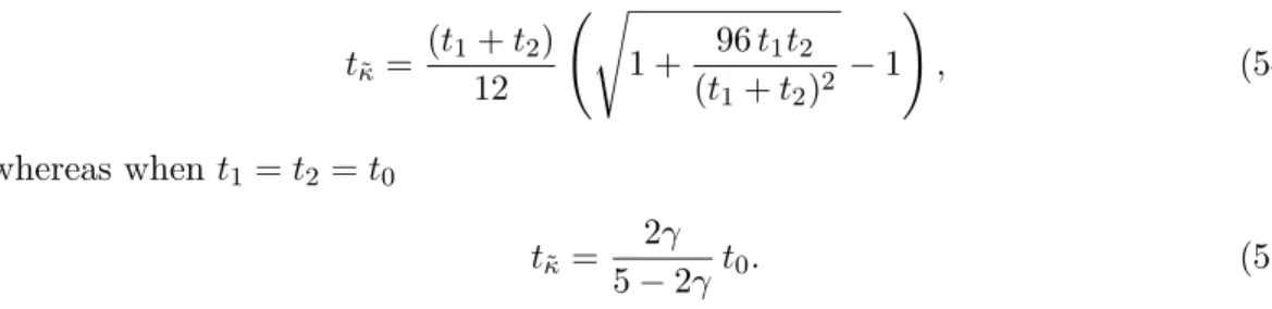
t˜κ=
(t1+t2)
12
s
1 + 96t1t2 (t1+t2)2 −
1 !
, (54)
whereas when t1=t2 =t0
tκ˜ =
2γ
5−2γ t0. (55)
Interpretation of the qualitative behaviour. To conclude, the junction response ˜κ2norm
can forγ = 1 be expected to increase with scales when a single corner model of infinite extent constitutes a reasonable approximation. On the other hand, ˜κ2norm can be expected to decrease with scales when so much smoothing is applied that the overall shape of the object is substantially distorted (and neighbouring junctions interfere with each other or disappear altogether).
Hence, selecting scale levels (and spatial points) where ˜κ2norm assumes maxima over scales can be expected to give rise to scale levels in the intermediate scale range (where a finite extent junction model constitutes a reasonable approximation). In particular, this approach will lead to larger scale values for corners having large spatial extent, and prevent too fine scales from being selected at rounded junctions. 6.3 Experiments: Scale-space signatures in junction detection
Figure 9 illustrates these effects for syntheticL-junctions with varying degrees of dif-fuseness. It shows simulation experiments with scale-space signatures of ˜κnorm accu-mulated in two different ways: (i) a vertical signature obtained by computing ˜κnorm
diffuseL-junction path signatureκ˜norm vertical signatureκ˜norm
t0= 4.0
0 1 2 3 4 5 6
0 100000 200000 300000 400000 500000
0 1 2 3 4 5 6
0 50000 100000 150000 200000 250000
t0= 64.0
0 1 2 3 4 5 6
0 50000 100000 150000 200000 250000
0 1 2 3 4 5 6
0 20000 40000 60000 80000 100000 120000
Figure 9: Scale-space signatures of ˜κnorm for synthetic L-junctions with different degrees of diffuseness (top t= 4.0, bottomt = 64.0). (left) original grey-level image, (middle) path signature of ˜κnormaccumulated by tracking a spatial maximum in ˜κnormacross scales, (right) vertical signature of ˜κnormaccumulated at the central point.
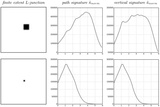
finite extent L-junction path signatureκ˜norm vertical signatureκ˜norm
0 1 2 3 4 5 6
0 100000 200000 300000 400000 500000
0 1 2 3 4 5 6
50000 100000 150000 200000 250000 300000
0 1 2 3 4 5 6
0 50000 100000 150000 200000 250000 300000
0 1 2 3 4 5 6
0 50000 100000 150000 200000 250000 300000
Figure 10: Scale-space signatures of ˜κnorm for diffuse L-junctions (t0 = 1.0) of different spatial extent (1/4 and 1/16 of the image size). (left) original grey-level image, (middle) path signature of ˜κnormaccumulated by tracking a spatial maximum in ˜κnormacross scales, (right) vertical signature of ˜κnormaccumulated at the central point.
at the fixed central point at different scales, and (ii) a path signature obtained by tracking the spatial extremum in ˜κnorm across scales. As can be seen, the qualitative behaviour is in agreement with the approximate analysis in previous section—with increasing degree of diffuseness the values of ˜κnorm become smaller at fine scales.
Figure 10 shows the result of replacing the infinite extent L-junction model by junction models of finite size. Observe that the peak in the signature is assumed at finer scales when the spatial extent of the junction is decreased. In other words, the scale at which the maximum over scales is assumed indicates the spatial extent (the size) of the region for which a junction model is consistent with the grey-level data (in agreement with the suggested scale selection principle).
Figure 11 gives a three-dimensional illustration of this junction detector with automatic scale selection. It shows scale-space maxima of ˜κ2norm computed from a synthetic image containing corner structures at different scales. The original grey-level image is shown in the ground plane, and each scale-space maximum has been graphically visualized by a sphere centered at the position (x0; t0) in scale-space
at which the scale-space maximum was assumed. (Hence, the height over the image plane reflects the selected scale.) Observe how the large scale corner as a whole gives rise to a response at coarse scales, whereas the superimposed corner structures of smaller size give rise to scale-space maxima at finer scales.
More results on corner detection, including a complementary mechanism for ac-curate corner localization, are presented in section 7.
7 Feature localization with automatic scale selection
The scale selection methodology presented so far applies to the detection of image features, and the role of the scale selection mechanism is to estimate the approxi-mate size of the image structures the feature detector responds to. Whereas this ap-proach provides a conceptually simple way to express various feature detectors, such as a junction detector, which automatically adapts its scale levels to the local image structure, it is not guaranteed that the spatial positions of the scale-space maxima constitute accurate estimates of the corner locations. The local maxima over scales may be assumed at rather coarse scales, where the drift due to scale-space smoothing is substantial and adjacent features may interfere with each other. For this reason, it is natural to complement the initial feature detection step by an explicit feature localization stage.
The subject of this section is show how mechanism for automatic scale selection can be formulated in this context,by minimizing normalized measures of inconsistency over scales.
7.1 Corner localization by local consistency
Second stage computation of localization estimate. Given an approximate estimate
x0 of the location and the size s of a corner (computed according to section 6),
an improved estimate of the corner position can be computed as follows: Following (F¨orstner and G¨ulch 1987), consider at every pointx0 ∈R2 in a neighbourhood of a junction candidate x0, the line lx0 perpendicular to the gradient vector (∇L)(x0) = (Lx1, Lx2)T(x0) at that point:
Figure 11: Three-dimensional view of scale-space maxima of ˜κ2norm computed for a large scale corner with superimposed corner structures at finer scales. Observe that a coarse scale response is obtained for the large scale corner structure as a whole, whereas the superimposed corner structures of smaller size give rise to scale-space maxima at finer scales.
Then, minimize the perpendicular distance to all lines lx0 in a neighbourhood of x0,
i.e.determine the pointx∈R2 that minimizes min
x∈R2 Z
x0∈R2
(Dx0(x))2wx0(x0)dx0 (57)
for some window function wx0:R2 →Rcentered at the candidate junction x0.
Mini-mizing this expression corresponds to finding the pointxthat minimizes the weighted integral of the squares of the distances from x to all lx0 in the neighbourhood, see figure 12. (Dx0(x) is distance fromx tolx0 multiplied by the gradient magnitude, and the window function implies that stronger weights are given to points in a neighbour-hood of x0.) The overall intention of this formulation is that for an image pattern
containing a junction, the point x that minimizes (57) should constitute a better estimate of the projection of the physical junction than x0.
Explicit solution in terms of local image statistics. An attractive property of the for-mulation in (57) is that it allows for a compact closed-form solution. After expansion, it can be written
min x∈R2
Z x0∈R2
new estimate, x
candidate junction,x0
n(x0) =∇L(x0) x0
Figure 12:Minimizing (57) basically corresponds to finding the pointxthat minimizes the distance to all edge tangents in a neighbourhood of the given candidate junction pointx0.
and the minimization problem be expressed as a standard least squares problem min
x∈R2 x
TA x−2xTb+c ⇐⇒ A x=b, (59)
where x = (x1, x2)T, and A, b, and c are determined by the local statistics of the
gradient directions in a neighbourhood ofx0,
A= Z
x0∈R2
(∇L)(x0) (∇L)T(x0)wx0(x0)dx0, (60)
b= Z
x0∈R2
(∇L)(x0) (∇L)T(x0)x0wx0(x0)dx0, (61)
c= Z
x0∈R2
x0T (∇L)(x0) (∇L)T(x0)x0wx0(x0)dx0. (62) Provided that the 2×2 matrix A is non-singular, the minimum value is given by
dmin = min x∈R2 x
TA x−2xTb+c=c−bTA−1b, (63)
and the point x that minimizes (57) is x = A−1b. Hence, an improved localization estimate can be computed directly from image measurements.
7.2 Automatic selection of localization scales
The formulation in previous section however, leaves two major problems open: How to choose the window functionwx0, and the scale(s) for computing the gradient vectors.
• The problem of choosing the weighting function is a special case of a common scale problem in least squares estimation: Over what spatial region should the fitting be performed? Clearly, it should be large enough such that statistics of gradient directions is accumulated over a sufficiently large neighbourhood around the candidate junction. Nevertheless, the region must not be so large that interfering structures corresponding to other junctions are included.
• The second scale problem, on the other hand, is of a slightly different nature than the previous ones—it concerns what scales should be used for localizing image structures. Previously, in this paper, only the problem ofdetecting image structures has been treated.