A First Course
in Structural
Equation Modeling
T
ENKO
R
AYKOV
• G
EORGE
A. M
ARCOULIDES
A First Course
in Structural
Equation Modeling
A First Course
in
Structural Equation Modeling
Second Edition
A First Course
in
Structural Equation Modeling
Second Edition
Tenko Raykov
Michigan State University
and
George A. Marcoulides
California State University, Fullerton
LAWRENCE ERLBAUM ASSOCIATES, PUBLISHERS
All rights reserved. No part of this book may be reproduced in any form, by photostat, microform, retrieval system, or any other means, without prior written permission of the publisher.
Lawrence Erlbaum Associates, Inc., Publishers 10 Industrial Avenue
Mahwah, New Jersey 07430 www.erlbaum.com
Cover design by Kathryn Houghtaling Lacey Library of Congress Cataloging-in-Publication Data Raykov, Tenko.
A first course in structural equation modeling—2nd ed. / Tenko Raykov and George A. Marcoulides.
p. cm.
Includes bibliographical references and index. ISBN 0-8058-5587-4 (cloth : alk. paper)
ISBN 0-8058-5588-2 (pbk. : alk. paper)
1. Multivariate analysis. 2. Social sciences—Statistical methods. I. Marcoulides, George A. II. Title.
2006
—dc22 2005000000
CIP Books published by Lawrence Erlbaum Associates are printed on acid-free paper, and their bindings are chosen for strength and durability. Printed in the United States of America
Contents
Preface
vii1
Fundamentals of Structural Equation Modeling
1What Is Structural Equation Modeling? 1 Path Diagrams 8
Rules for Determining Model Parameters 17 Parameter Estimation 22
Parameter and Model Identification 34 Model-Testing and -Fit Evaluation 38 Appendix to Chapter 1 52
2
Getting to Know the EQS, LISREL, and M
plus
Programs
55Structure of Input Files for SEM Programs 55 Introduction to the EQS Notation and Syntax 57 Introduction to the LISREL Notation and Syntax 64 Introduction to the MplusNotation and Syntax 73
3
Path Analysis
77What Is Path Analysis? 77 Example Path Analysis Model 78 EQS, LISREL, and MplusInput Files 80 Modeling Results 84
Testing Model Restrictions in SEM 100
Model Modifications 109 Appendix to Chapter 3 114
4
Confirmatory Factor Analysis
116What Is Factor Analysis? 116
An Example Confirmatory Factor Analysis Model 118 EQS, LISREL, and MplusCommand Files 120
Modeling Results 124
Testing Model Restrictions: True Score Equivalence 140 Appendix to Chapter 4 145
5
Structural Regression Models
147What Is a Structural Regression Model? 147 An Example Structural Regression Model 148 EQS, LISREL, and MplusCommand Files 150 Modeling Results 153
Factorial Invariance Across Time In Repeated Measure Studies 162
Appendix to Chapter 5 173
6
Latent Change Analysis
175What is Latent Change Analysis? 175
Simple One-Factor Latent Change Analysis Model 177 EQS, LISREL, and MplusCommand Files for a One-Factor LCA
Model 181
Modeling Results, One-Factor LCA Model 187 Level and Shape Model 192
EQS, LISREL, and MplusCommand Files, Level and Shape
Model 195
Modeling Results for a Level and Shape Model 197 Studying Correlates and Predictors of Latent Change 201 Appendix to Chapter 6 222
Epilogue
225References
227Author Index
233Preface to the Second Edition
The idea when working on the second edition of this book was to provide a current text for an introductory structural equation modeling (SEM) course similar to the ones we teach for our departments at Michigan State Univer-sity and California State UniverUniver-sity, Fullerton. Our goal is to present an up-dated, conceptual and nonmathematical introduction to the increasingly popular in the social and behavioral sciences SEM methodology. The read-ership we have in mind with this edition consists of advanced undergradu-ate students, graduundergradu-ate students, and researchers from any discipline, who have limited or no previous exposure to this analytic approach. Like before, in the past six years since the appearance of the first edition we could not lo-cate a book that we thought would be appropriate for such an audience and course. Most of the available texts have what we see as significant limita-tions that may preclude their successful use in an introductory course. These books are either too technical for beginners, do not cover in suffi-cient breadth and detail the fundamentals of the methodology, or intermix fairly advanced issues with basic ones.
This edition maintains the previous goal of providing an alternative at-tempt to offer a first course in structural equation modeling at a coherent introductory level. Similarly to the first edition, there are no special prereq-uisites beyond a course in basic statistics that included coverage of regres-sion analysis. We frequently draw a parallel between aspects of SEM and their apparent analogs in regression, and this prior knowledge is both help-ful and important. In the main text, there are only a few mathematical for-mulas used, which are either conceptual or illustrative rather than computational in nature. In the appendixes to most of the chapters, we give the readers a glimpse into some formal aspects of topics discussed in the
pertinent chapter, which are directed at the mathematically more sophisti-cated among them. While desirable, the thorough understanding and mastery of these appendixes are not essential for accomplishing the main aims of the book.
The basic ideas and methods for conducting SEM as presented in this text are independent of particular software. We illustrate discussed model classes using the three apparently most widely circulated programs—EQS, LISREL, and Mplus. With these illustrations, we only aim at providing read-ers with information as to how to use these software, in terms of setting up command files and interpreting resulting output; we do not intend to imply any comparison between these programs or impart any judgment on rela-tive strengths or limitations. To emphasize this, we discuss their input and output files in alphabetic order of software name, and in the later chapters use them in turn.
The goal of this text, however, is going well beyond discussion of com-mand file generation and output interpretation for these SEM programs. Our primary aim is to provide the readers with an understanding of fundamental aspects of structural equation modeling, which we find to be of special rele-vance and believe will help them profitably utilize this methodology. Many of these aspects are discussed in Chapter 1, and thus a careful study of it before proceeding with the subsequent chapters and SEM applications is strongly recommended especially for newcomers to this field.
Due to the targeted audience of mostly first-time SEM users, many impor-tant advanced topics could not be covered in the book. Anyone interested in such topics could consult more advanced SEM texts published throughout the past 15 years or so (information about a score of them can be obtained from http://www.erlbaum.com/) and the above programs’ manuals. We view our book as a stand-alone precursor to these advanced texts.
Our efforts to produce this book would not have been successful without the continued support and encouragement we have received from many scholars in the SEM area. We feel particularly indebted to Peter M. Bentler, Michael W. Browne, Karl G. Jöreskog, and Bengt O. Muthén for their path-breaking and far-reaching contributions to this field as well as helpful dis-cussions and instruction throughout the years. In many regards they have profoundly influenced our understanding of SEM. We would also like to thank numerous colleagues and students who offered valuable comments and criticism on earlier drafts of various chapters as well as the first edition. For assistance and support, we are grateful to all at Lawrence Erlbaum Asso-ciates who were involved at various stages in the book production process. The second author also wishes to extend a very special thank you to the fol-lowing people for their helpful hand in making the completion of this pro-ject a possibility: Dr. Keith E. Blackwell, Dr. Dechen Dolkar, Dr. Richard E. Loyd, and Leigh Maple along with the many other support staff at the UCLA
and St. Jude Medical Centers. Finally, and most importantly, we thank our families for their continued love despite the fact that we keep taking on new projects. The first author wishes to thank Albena and Anna; the second author wishes to thank Laura and Katerina.
—Tenko Raykov East Lansing, Michigan —George A. Marcoulides Fullerton, California
Fundamentals of Structural
Equation Modeling
WHAT IS STRUCTURAL EQUATION MODELING?
Structural equation modeling (SEM) is a statistical methodology used by so-cial, behavioral, and educational scientists as well as biologists, economists, marketing, and medical researchers. One reason for its pervasive use in many scientific fields is that SEM provides researchers with a comprehen-sive method for the quantification and testing of substantive theories. Other major characteristics of structural equation models are that they explicitly take into account measurement error that is ubiquitous in most disciplines, and typically contain latent variables.
Latent variablesare theoretical or hypothetical constructs of major im-portance in many sciences, or alternatively can be viewed as variables that do not have observed realizations in a sample from a focused population. Hence, latent are such variables for which there are no available observa-tions in a given study. Typically, there is no direct operational method for measuring a latent variable or a precise method for its evaluation. Neverthe-less, manifestations of a latent construct can be observed by recording or measuring specific features of the behavior of studied subjects in a particu-lar environment and/or situation. Measurement of behavior is usually car-ried out using pertinent instrumentation, for example tests, scales, self-reports, inventories, or questionnaires. Once studied constructs have been assessed, SEM can be used to quantify and test plausibility of hypothetical assertions about potential interrelationships among the constructs as well as their relationships to measures assessing them. Due to the mathematical complexities of estimating and testing these relationships and assertions,
computer software is a must in applications of SEM. To date, numerous programs are available for conducting SEM analyses. Software such as AMOS (Arbuckle & Wothke, 1999), EQS (Bentler, 2004), LISREL (Jöreskog & Sörbom, 1993a, 1993b, 1993c, 1999), Mplus(Muthén & Muthén, 2004), SAS PROC CALIS (SAS Institute, 1989), SEPATH (Statistica, 1998), and RAMONA (Browne & Mels, 2005) are likely to contribute in the coming years to yet a further increase in applications of this methodology. Although these programs have somewhat similar capabilities, LISREL and EQS seem to have historically dominated the field for a number of years (Marsh, Balla, & Hau, 1996); in addition, more recently Mplushas substantially gained in popularity among social, behavioral, and educational researchers. For this reason, and because it would be impossible to cover every program in rea-sonable detail in an introductory text, examples in this book are illustrated using only the LISREL, EQS, and Mplussoftware.
The termstructural equation modelingis used throughout this text as a generic notion referring to various types of commonly encountered mod-els. The following are some characteristics of structural equation modmod-els. 1. The models are usually conceived in terms of not directly measur-able, and possibly not (very) well-defined, theoretical or hypothetical constructs. For example, anxiety, attitudes, goals, intelligence, motiva-tion, personality, reading and writing abilities, aggression, and socioeco-nomic status can be considered representative of such constructs.
2. The models usually take into account potential errors of measure-ment in all observed variables, in particular in the independent (predic-tor, explanatory) variables. This is achieved by including an error term for each fallible measure, whether it is an explanatory or predicted vari-able. The variances of the error terms are, in general, parameters that are estimated when a model is fit to data. Tests of hypotheses about them can also be carried out when they represent substantively meaningful asser-tions about error variables or their relaasser-tionships to other parameters.
3. The models are usually fit to matrices of interrelationship indices— that is, covariance or correlation matrices—between all pairs of ob-served variables, and sometimes also to variable means.1
1
It can be shown that the fit function minimized with the maximum likelihood (ML) method used in a large part of current applications of SEM, is based on the likelihood function of the raw data (e.g., Bollen, 1989; see also section “Rules for Determining Model Parame-ters”). Hence, with multinormality, a structural equation model can be considered indirectly fitted to the raw data as well, similarly to models within the general linear modeling frame-work. Since this is an introductory book, however, we emphasize here the more direct process of fitting a model to the analyzed matrix of variable interrelationship indices, which can be viewed as the underlying idea of the most general asymptotically distribution-free method of model fitting and testing in SEM. The maximization of the likelihood function for the raw data is equivalent to the minimization of the fit function with the ML method,FML, which quantifies
This list of characteristics can be used to differentiate structural equation models from what we would like to refer to in this book as classical linear modeling approaches. These classical approaches encompass regression analysis, analysis of variance, analysis of covariance, and a large part of multivariate statistical methods (e.g., Johnson & Wichern, 2002; Marcoulides & Hershberger, 1997). In the classical approaches, typically models are fit to raw data and no error of measurement in the independent variables is assumed.
Despite these differences, an important feature that many of the classical approaches share with SEM is that they are based on linear models. There-fore, a frequent assumption made when using the SEM methodology is that the relationships among observed and/or latent variables are linear (al-though modeling nonlinear relationships is increasingly gaining popularity in SEM; see Schumacker & Marcoulides, 1998; Muthén & Muthén, 2004; Skrondal & Rabe-Hesketh, 2004). Another shared property between classi-cal approaches and SEM is model comparison. For example, the well-knownFtest for comparing a less restricted model to a more restricted model is used in regression analysis when a researcher is interested in test-ing whether to drop from a considered model (prediction equation) one or more independent variables. As discussed later, the counterpart of this test in SEM is the difference in chi-square values test, or its asymptotic equiva-lents in the form of Lagrange multiplier or Wald tests (e.g., Bentler, 2004). More generally, the chi-square difference test is used in SEM to examine the plausibility of model parameter restrictions, for example equality of factor loadings, factor or error variances, or factor variances and covariances across groups.
Types of Structural Equation Models
The following types of commonly used structural equation models are con-sidered in this book.
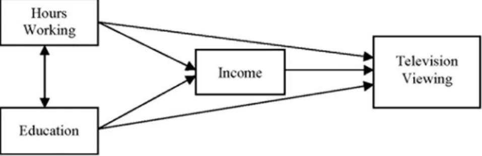
1.Path analysis models.Path analysis models are usually conceived of only in terms of observed variables. For this reason, some researchers do not consider them typical SEM models. We believe that path analysis models are worthy of discussion within the general SEM framework be-cause, although they only focus on observed variables, they are an im-portant part of the historical development of SEM and in particular use the same underlying idea of model fitting and testing as other SEM mod-els. Figure 1 presents an example of a path analysis model examining the effects of several explanatory variables on the number of hours spent
the distance between that matrix and the one reproduced by the model (see section “Rules for Determining Model Parameters” and the Appendix to this chapter).
watching television (see section “Path Diagrams” for a complete list and discussion of the symbols that are commonly used to graphically repre-sent structural equation models).
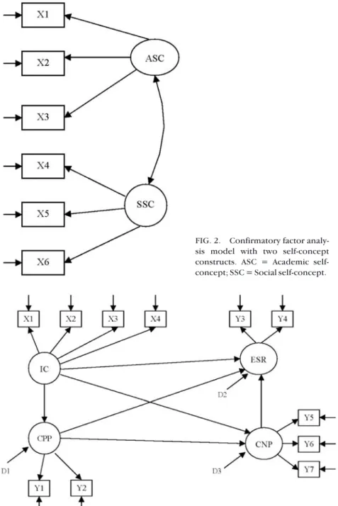
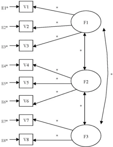
2.Confirmatory factor analysis models.Confirmatory factor analy-sis models are frequently employed to examine patterns of interrela-tionships among several latent constructs. Each construct included in the model is usually measured by a set of observed indicators. Hence, in a confirmatory factor analysis model no specific directional relation-ships are assumed between the constructs, only that they are poten-tially correlated with one another. Figure 2 presents an example of a confirmatory factor analysis model with two interrelated self-concept constructs (Marcoulides & Hershberger, 1997).
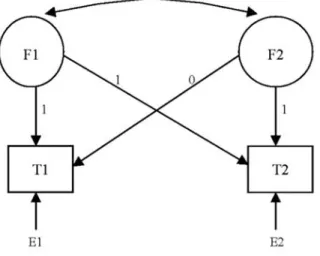
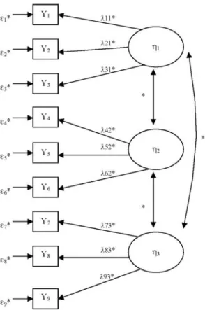
3.Structural regression models.Structural regression models resem-ble confirmatory factor analysis models, except that they also postulate particular explanatory relationships among constructs (latent regres-sions) rather than these latent variables being only interrelated among themselves. The models can be used to test or disconfirm theories about explanatory relationships among various latent variables under investi-gation. Figure 3 presents an example of a structural regression model of variables assumed to influence returns of promotion for faculty in higher education (Heck & Johnsrud, 1994).
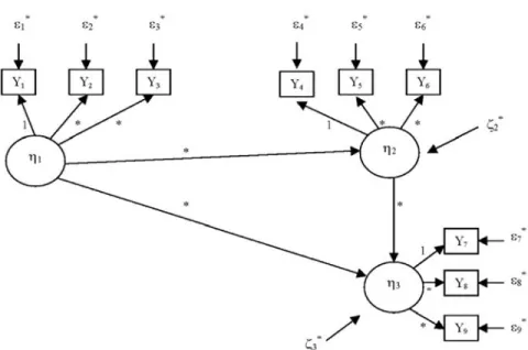
4.Latent change models.Latent change models, often also called la-tent growth curve models or lala-tent curve analysis models (e.g., Bollen & Curran, 2006; Meredith & Tisak, 1990), represent a means of studying change over time. The models focus primarily on patterns of growth, de-cline, or both in longitudinal data (e.g., on such aspects of temporal change as initial status and rates of growth or decline), and enable
re-FIG. 1. Path analysis model examining the effects of some variables on television viewing. Hours Working = Average weekly working hours; Education = Number of completed school years; Income = Yearly gross income in dollars; Television Viewing = Average daily number of hours spent watching television.
5
sis model with two self-concept constructs. ASC = Academic self-concept; SSC = Social self-concept.
FIG. 3. Structural regression model of variables influencing return to promotion. IC = Individual characteristics; CPP = Characteristics of prior positions; ESR = Eco-nomic and social returns to promotion; CNP = Characteristics of new positions.
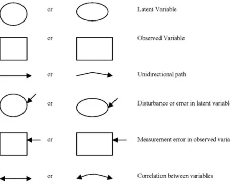
searchers to examine both intraindividual temporal development and interindividual similarities and differences in its patterns. The models can also be used to evaluate the relationships between patterns of change and other personal characteristics. Figure 4 presents the idea of a simple example of a two-factor growth model for two time points, al-though typical applications of these models occur in studies with more than two repeated assessments as discussed in more detail in Chapter 6.
When and How Are Structural Equation Models Used?
Structural equation models can be utilized to represent knowledge or hy-potheses about phenomena studied in substantive domains. The models are usually, and should best be, based on existing or proposed theories that describe and explain phenomena under investigation. With their unique feature of explicitly modeling measurement error, structural equation models provide an attractive means for examining such phenomena. Once a theory has been developed about a phenomenon of interest, the theory can be tested against empirical data using SEM. This process of testing is of-ten calledconfirmatory modeof SEM applications.
A related utilization of structural models is construct validation. In these applications, researchers are interested mainly in evaluating the ex-tent to which particular instruments actually measure a laex-tent variable they are supposed to assess. This type of SEM use is most frequently employed when studying the psychometric properties of a given measurement device (e.g., Raykov, 2004).
Structural equation models are also used for theory development pur-poses. Intheory development, repeated applications of SEM are carried
FIG. 4. A simple latent change model.
out, often on the same data set, in order to explore potential relationships between variables of interest. In contrast to the confirmatory mode of SEM applications, theory development assumes that no prior theory exists—or that one is available only in a rudimentary form—about a phenomenon under investigation. Since this utilization of SEM contributes both to the clarification and development of theories, it is commonly referred to as
exploratory mode of SEM applications. Due to this development fre-quently occurring based on a single data set (single sample from a studied population), results from such exploratory applications of SEM need to be interpreted with great caution (e.g., MacCallum, 1986). Only when the findings are replicated across other samples from the same population, can they be considered more trustworthy. The reason for this concern stems mainly from the fact that results obtained by repeated SEM applica-tions on a given sample may be capitalizing on chance factors having lead to obtaining the particular data set, which limits generalizability of results beyond that sample.
Why Are Structural Equation Models Used?
A main reason that structural equation models are widely employed in many scientific fields is that they provide a mechanism for explicitly taking into account measurement error in the observed variables (both depend-ent and independdepend-ent) in a given model. In contrast, traditional regression analysis effectively ignores potential measurement error in the explanatory (predictor, independent) variables. As a consequence, regression results can be incorrect and possibly entail misleading substantive conclusions.
In addition to handling measurement error, SEM also enables researchers to readily develop, estimate, and test complex multivariable models, as well as to study both direct and indirect effects of variables involved in a given model.
Direct effectsare the effects that go directly from one variable to another vari-able.Indirect effectsare the effects between two variables that are mediated by one or more intervening variables that are often referred to as a mediating vari-able(s) or mediator(s). The combination of direct and indirect effects makes up thetotal effectof an explanatory variable on a dependent variable. Hence, if an indirect effect does not receive proper attention, the relationship between two variables of concern may not be fully considered. Although regression analysis can also be used to estimate indirect effects—for example by regress-ing the mediatregress-ing on the explanatory variable, then the effect variable on the mediator, and finally multiplying pertinent regression weights—this is strictly appropriate only when there are no measurement errors in the involved pre-dictor variables. Such an assumption, however, is in general unrealistic in em-pirical research in the social and behavioral sciences. In addition, standard errors for relevant estimates are difficult to compute using this sequential
ap-plication of regression analysis, but are quite straightforwardly obtained in SEM applications for purposes of studying indirect effects.
What Are the Key Elements of Structural Equation Models?
The key elements of essentially all structural equation models are their param-eters (often referred to as model paramparam-eters or unknown paramparam-eters). Model parameters reflect those aspects of a model that are typically unknown to the researcher, at least at the beginning of the analyses, yet are of potential interest to him or her.Parameteris a generic term referring to a characteristic of a pop-ulation, such as mean or variance on a given variable, which is of relevance in a particular study. Although this characteristic is difficult to obtain, its inclusion into one’s modeling considerations can be viewed as essential in order to facili-tate understanding of the phenomenon under investigation. Appropriate sam-ple statistics are used to estimate parameter(s). In SEM, the parameters are unknown aspects of a phenomenon under investigation, which are related to the distribution of the variables in an entertained model. The parameters are estimated, most frequently from the sample covariance matrix and possibly observed variable means, using specialized software.
The presence of parameters in structural equation models should not pose any difficulties to a newcomer to the SEM field. The well-known regres-sion analysis models are also built upon multiple parameters. For example, the partial regression coefficients (or slope), intercept, and standard error of estimate are parameters in a multiple (or simple) regression model. Simi-larly, in a factorial analysis of variance the main effects and interaction(s) are model parameters. In general, parameters are essential elements of statistical models used in empirical research. The parameters reflect unknown aspects of a studied phenomenon and are estimated by fitting the model to sampled data using particular optimality criteria, numeric routines, and specific soft-ware. The topic of structural equation model parameters, along with a com-plete description of the rules that can be used to determine them, are discussed extensively in the following section “Parameter Estimation.”
PATH DIAGRAMS
One of the easiest ways to communicate a structural equation model is to draw a diagram of it, referred to aspath diagram, using special graphical notation. A path diagram is a form of graphical representation of a model under consideration. Such a diagram is equivalent to a set of equations de-fining a model (in addition to distributional and related assumptions), and is typically used as an alternative way of presenting a model pictorially. Path diagrams not only enhance the understanding of structural equation mod-els and their communication among researchers with various backgrounds,
but also substantially contribute to the creation of correct command files to fit and test models with specialized programs. Figure 5 displays the most commonly used graphical notation for depicting SEM models, which is de-scribed in detail next.
Latent and Observed Variables
One of the most important initial issues to resolve when using SEM is the distinction between observed variables and latent variables.Observed vari-ablesare the variables that are actually measured or recorded on a sample of subjects, such as manifested performance on a particular test or the answers to items or questions in an inventory or questionnaire. The term manifest variables is also often used for observed variables, to stress the fact that these are the variables that have actually been measured by the re-searcher in the process of data collection. In contrast,latent variablesare typically hypothetically existing constructs of interest in a study. For exam-ple, intelligence, anxiety, locus of control, organizational culture, motiva-tion, depression, social support, math ability, and socioeconomic status can all be considered latent variables. The main characteristic of latent
ables is that they cannot be measured directly, because they are not directly observable . Hence, only proxies for them can be obtained using specifically developed measuring instruments, such as tests, inventories, self-reports, testlets, scales, questionnaires, or subscales. These proxies are the indica-tors of the latent constructs or, in simple terms, their measured aspects. For example, socioeconomic status may be considered to be measured in terms of income level, years of education, bank savings, type of occupation. Simi-larly, intelligence may be viewed as manifested (indicated) by subject per-formance on reasoning, figural relations, and culture-fair tests. Further, mathematical ability may be considered indicated by how well students do on algebra, geometry, and trigonometry tasks. Obviously, it is quite com-mon for manifest variables to be fallible and unreliable indicators of the un-observable latent constructs of actual interest to a social or behavioral researcher. If a single observed variable is used as an indicator of a latent variable, it is most likely that the manifest variable will generally contain quite unreliable information about that construct. This information can be considered to be one-sided because it reflects only one aspect of the sured construct, the side captured by the observed variable used for its mea-surement. It is therefore generally recommended that researchers employ multiple indicators (preferably more than two) for each latent variable in order to obtain a much more complete and reliable picture of it than that provided by a single indicator. There are, however, instances in which a sin-gle observed variable may be a fairly good indicator of a latent variable, e.g., the total score on the Stanford-Binet Intelligence Test as a measure of the construct of intelligence.
The discussed meaning of latent variable could be referred to as a tradi-tional, classical, or ‘psychometric’ conceptualization. This treatment of latent variable reflects a widespread understanding of unobservable constructs across the social and behavioral disciplines as reflecting proper subject charac-teristics that cannot be directly measured but (a) could be meaningfully as-sumed to exist separately from their measures without contradicting observed data, and (b) allow the development and testing of potentially far-reaching substantive theories that contribute significantly to knowledge accumulation in these sciences. This conceptualization of latent variable can be traced back perhaps to the pioneering work of the English psychologist Charles Spearman in the area of factor analysis around the turn of the 20th century (e.g., Spearman, 1904), and has enjoyed wide acceptance in the social and behav-ioral sciences over the past century. During the last 20 years or so, however, de-velopments primarily in applied statistics have suggested the possibility of extending this traditional meaning of the concept of latent variable (e.g., Muthén, 2002; Skrondal & Rabe-Hesketh, 2004). According to what could be referred to as its modern conceptualization, any variable without observed re-alizations in a studied sample from a population of interest can be considered
a latent variable. In this way, as we will discuss in more detail in Chapter 6, pat-terns of intraindividual change (individual growth or decline trajectories) such as initial true status or true change across the period of a repeated measure study, can also be considered and in fact profitably used as latent variables. As another, perhaps more trivial example, the error term in a simple or multiple regression equation or in any statistical model containing a residual, can also be viewed as a latent variable. A common characteristic of these examples is that individual realizations (values) of the pertinent latent variables are con-ceptualized in a given study or modeling approach—e.g., the individual initial true status and overall change, or error score—which realizations however are not observed (see also Appendix to this chapter).2
This extended conceptualization of the notion of latent variable obvi-ously includes as a special case the traditional, ‘psychometric’ understand-ing of latent constructs, which would be sufficient to use in most chapters of this introductory book. The benefit of adopting the more general, modern understanding of latent variable will be seen in the last chapter of the book. This benefit stems from the fact that the modern view provides the opportu-nity to capitalize on highly enriching developments in applied statistics and numerical analysis that have occurred over the past couple of decades, which allow one to consider the above modeling approaches, including SEM, as examples of a more general, latent variable modeling methodology (e.g., Muthén, 2002).
Squares and Rectangles, Circles and Ellipses
Observed and latent variables are represented in path diagrams by two dis-tinct graphical symbols. Squares or rectangles are used for observed vari-ables, and circles or ellipses are employed for latent variables. Observed variables are usually labeled sequentially (e.g., X1,X2,X3), with the label centered in each square or rectangle. Latent variables can be abbreviated ac-cording to the construct they present (e.g.,SESfor socioeconomic status) or just labeled sequentially (e.g.,F1,F2;Fstanding for “factor”) with the name or label centered in each circle or ellipse.
Paths and Two-Way Arrows
Latent and observed variables are connected in a structural equation model in order to reflect a set of propositions about a studied phenomenon,
2Further, individual class or cluster membership in a latent class model or cluster analysis
can be seen as a latent variable. Membership to a constituent in a finite mixture distribution may also be viewed as a latent variable. Similarly, the individual values of random effects in multi-level (hierarchical) or simpler variance component models can be considered scores on latent dimensions as well.
which a researcher is interested in examining (testing) using SEM. Typi-cally, the interrelationships among the latent as well as the latent and ob-served variables are the main focus of study. These relationships are represented graphically in a path diagram by one-way and two-way arrows. The one-way arrows, also frequently called paths, signal that a variable at the end of the arrow is explained in the model by the variable at the begin-ning of the arrow. One-way arrows, or paths, are usually represented by straight lines, with arrowheads at the end of the lines. Such paths are often interpreted as symbolizing causal relationships—the variable at the end of the arrow is assumed according to the model to be the effect and the one at the beginning to be the cause. We believe that such inferences should not be made from path diagrams without a strong rationale for doing so. For in-stance, latent variables are oftentimes considered to be causes for their indi-cators; that is, the measured or recorded performance is viewed to be the effect of the presence of a corresponding latent variable. We generally ab-stain from making causal interpretations from structural equation models except possibly when the variable considered temporally precedes another one, in which case the former could be interpreted as the cause of the one occurring later (e.g., Babbie, 1992, chap. 1; Bollen, 1989, chap. 3). Bollen (1989) lists three conditions that should be used to establish a causal rela-tion between variables—isolarela-tion, associarela-tion, and direcrela-tion of causality. While association may be easier to examine, it is quite difficult to ensure that a cause and effect have been isolated from all other influences. For this reason, most researchers consider SEM models and the causal relations within them only as approximations to reality that perhaps can never really be proved, but rather only disproved or disconfirmed.
In a path diagram, two-way arrows (sometimes referred to as two-way paths) are used to represent covariation between two variables, and signal that there is an association between the connected variables that is not as-sumed in the model to be directional. Usually two-way arrows are graphi-cally represented as curved lines with an arrowhead at each end. A straight line with arrowheads at each end is also sometimes used to symbolize a cor-relation between variables. Lack of space may also force researchers to even represent a one-way arrow by a curved rather than a straight line, with an ar-rowhead attached to the appropriate end (e.g., Fig. 5). Therefore, when first looking at a path diagram of a structural equation model it is essential to determine which of the straight or curved lines have two arrowheads and which only one.
Dependent and Independent Variables
In order to properly conceptualize a proposed model, there is another dis-tinction between variables that is of great importance—the differentiation
between dependent and independent variables. Dependent variables are those that receive at least one path (one-way arrow) from another variable in the model. Hence, when an entertained model is represented as a set of equations (with pertinent distributional and related assumptions), each de-pendent variable will appear in the left-hand side of an equation. Independ-ent variables are variables that emanate paths (one-way arrows), but never receive a path; that is, no independent variable will appear in the left-hand side of an equation, in that system of model equations. Independent vari-ables can be correlated among one another, i.e., connected in the path dia-gram by two-way arrows. We note that a dependent variable may act as an independent variable with respect to another variable, but this does not change its dependent-variable status. As long as there is at least one path (one-way arrow) ending at the variable, it is a dependent variable no matter how many other variables in the model are explained by it.
In the econometric literature, the terms exogenous variables and endo-genous variables are also frequently used for independent and dependent variables, respectively. (These terms are derived from the Greek words exo and endos, for being correspondingly of external origin to the system of variables under consideration, and of internal origin to it.) Regardless of the terms one uses, an important implication of the distinction between de-pendent and indede-pendent variables is that there are no two-way arrows connecting any two dependent variables, or a dependent with an inde-pendent variable, in a model path diagram. For reasons that will become much clearer later, the variances and covariances (and correlations) be-tween dependent variables, as well as covariances bebe-tween dependent and independent variables, are explained in a structural equation model in terms of its unknown parameters.
An Example Path Diagram of a Structural Equation Model
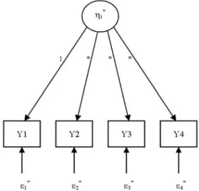
To clarify further the discussion of path diagrams, consider the factor analy-sis model displayed in Fig. 6. This model represents assumed relationships among Parental dominance, Child intelligence, and Achievement motiva-tion as well as their indicators.
As can be seen by examining Fig. 6, there are nine observed variables in the model. The observed variables represent nine scale scores that were ob-tained from a sample of 245 elementary school students. The variables are denoted by the labelsV1throughV9(usingVfor ‘observed Variable’). The la-tent variables (or factors) are Parental dominance, Child intelligence, and Achievement motivation. As latent variables (factors), they are denotedF1,
F2, andF3, respectively. The factors are each measured by three indicators, with each path in Fig. 6 symbolizing the factor loading of the observed vari-able on its pertinent latent varivari-able.
The two-way arrows in Fig. 6 designate the correlations between the la-tent variables (i.e., the factor correlations) in the model. There is also a re-sidual term attached to each manifest variable. The rere-siduals are denoted by
E (for Error), followed by the index of the variable to which they are at-tached. Each residual represents the amount of variation in the manifest variable that is due to measurement error or remains unexplained by varia-tion in the corresponding latent factor that variable loads on. The unex-plained variance is the amount of indicator variance unshared with the other measures of the particular common factor. In this text, for the sake of convenience, we will frequently refer to residuals as errors or error terms.
As indicated previously, it is instrumental for an SEM application to de-termine the dependent and the independent variables of a model under consideration. As can be seen in Fig. 6, and using the definition of error, there are a total of 12 independent variables in this model—these are the
FIG. 6. Example factor analysis model.F1= Parental dominance;F2= Child intelli-gence;F3= Achievement motivation.
three latent variables and nine residual terms. Indeed, if one were to write out the 9 model definition equations (see below), none of these 12 vari-ables will ever appear in the left-hand side of an equation. Note also that there are no one-way paths going into any independent variable, but there are paths leaving each one of them. In addition, there are three two-way ar-rows that connect the latent variables—they represent the three factor cor-relations. The dependent variables are the nine observed variables labeled
V1throughV9. Each of them receives two paths—(i) the path from the latent variable it loads on, which represents its factor loading; and (ii) the one from its residual term, which represents the error term effect.
First let us write down themodel definition equations. These are the re-lationships between observed and unobserved variables that formally de-fine the proposed model. Following Fig. 6, these equations are obtained by writing an equation for each observed variable in terms of how it is ex-plained in the model, i.e., in terms of the latent variable(s) it loads on and corresponding residual term. The following system of nine equations is ob-tained in this way (one equation per dependent variable):
V1=l1F1+E1,
V2=l2F1+E2,
V3=l3F1+E3,
V4=l4F2+E4,
V5=l5F2+E5, (1)
V6=l6F2+E6,
V7=l7F3+E7,
V8=l8F3+E8,
V9=l9F3+E9,
wherelltol9(Greek letterlambda) denote the nine factor loadings. In ad-dition, we make the usual assumptions of uncorrelated residuals among themselves and with the three factors, while the factors are allowed to be in-terrelated, and that the nine observed variables are normally distributed, like the three factors and the nine residuals that possess zero means. We note the similarity of these distributional assumptions with those typically made in the multiple regression model (general linear model), specifically the normality of its error term, having zero mean and being uncorrelated with the predictors (e.g., Tabachnick & Fidell, 2001).
According to the factor analysis model under consideration, each of the nine Equations in (1) represents the corresponding observed variable as the sum of the product of that variable’s factor loading with its pertinent fac-tor, and a residual term. Note that on the left-hand side of each equation there is only one variable, the dependent variable, rather than a combina-tion of variables, and also that no independent variable appears there.
Model Parameters and Asterisks
Another important feature of path diagrams, as used in this text, are the as-terisks associated with one-way and two-way arrows and independent vari-ables (e.g., Fig. 6). These asterisks are symbols of the unknown parameters and are very useful for understanding the parametric features of an enter-tained model as well as properly controlling its fitting and estimation pro-cess with most SEM programs. In our view, a satisfactory understanding of a given model can only then be accomplished when a researcher is able to lo-cate the unknown model parameters. If this is done incorrectly or arbi-trarily, there is a danger of ending up with a model that is unduly restrictive or has parameters that cannot be uniquely estimated. The latter problem-atic parameter estimation feature is characteristic of models that are un-identified—a notion discussed in greater detail in a later section—which are in general useless means of description and explanation of studied phe-nomena. The requirement of explicit understanding of all model parame-ters is quite unique to a SEM analysis but essential for meaningful utilization of pertinent software as well as subsequent model modification that is fre-quently needed in empirical research.
It is instructive to note that in difference to SEM, in regression analysis one does not really need to explicitly present the parameters of a fitted model, in particular when conducting this analysis with popular software. Indeed, suppose a researcher were interested in the following regression model aiming at predicting depression among college students:
Depression =a+b1Social-Support +
b2Intelligence +b3Age + Error,
(2)
where a is the intercept and b1, b2, and b3 are the partial regression weights (slopes), with the usual assumption of normal and homoscedas-tic error with zero mean, which is uncorrelated with the predictors. When this model is to be fitted with a major statistical package (e.g., SAS or SPSS), the researcher is not required to specifically definea,b1,b2and
b3, as well as the standard error of estimate, as the model parameters. This is due to the fact that unlike SEM, a regression analysis is routinely conducted in only one possible way with regard to the set of unknown parameters. Specifically, when a regression analysis is carried out, a re-searcher usually only needs to provide information about which mea-sures are to be used as explanatory variables and which as the dependent variables; the utilized software automatically determines then the model parameters, typically one slope per predictor (partial regression weight) plus an intercept for the fitted regression equation and the standard er-ror of estimate.
This automatic or default determination of model parameters does not generally work well in SEM applications and in our view should not be en-couraged when the aim is a meaningful utilization of SEM. We find it particu-larly important in SEM to explicitly keep track of the unknown parameters in order to understand and correctly set up the model one is interested in fitting as well as subsequently appropriately modify it if needed. Therefore, we strongly recommend that researchers always first determine (locate) the pa-rameters of a structural equation model they consider. Using default settings in SEM programs will not absolve a scientist from having to think carefully about this type of details for a particular model being examined. It is the re-searcher who must decide exactly how the model is defined, not the default features of a computer program used. For example, if a factor analytic model similar to the one presented in Fig. 6 is being considered in a study, one re-searcher may be interested in having all factor loadings as model parameters, whereas others may have reasons to view only a few of them as unknown. Furthermore, in a modeling session one is likely to be interested in several versions of an entertained model, which differ from one another only in the number and location of their parameters (see chapters 3 through 6 that also deal with such models). Hence, unlike routine applications of regression analysis, there is no single way of assuming unknown parameters without first considering a proposed structural equation model in the necessary de-tail that would allow one to determine its parameters. Since determination of unknown parameters is in our opinion particularly important in setting up structural equation models, we discuss it in detail next.
RULES FOR DETERMINING MODEL PARAMETERS
In order to correctly determine the parameters that can be uniquely esti-mated in a considered structural equation model, six rules can be used (cf. Bentler, 2004). The specific rationale behind them will be discussed in the next section of this chapter, which deals with parameter estimation. When the rules are applied in practice, for convenience no distinction needs to be made between the covariance and correlation of two independent variables (as they can be viewed equivalent for purposes of reflecting the degree of linear interrelationship between pairs of variables). For a given structural equation model, these rules are as follows.
Rule 1.All variances of independent variables are model parameters. For example, in the model depicted in Fig. 6 most of the variances of in-dependent variables are symbolized by asterisks that are associated with each error term (residual). Error terms in a path diagram are gen-erally attached to each dependent variable. For a latent dependent vari-able, an associated error term symbolizes the structural regression
disturbance that represents the variability in the latent variable unex-plained by the variables it is regressed upon in the model. For example, the residual terms displayed in Fig. 3,D1toD3, encompass the part of the corresponding dependent variable variance that is not accounted for by the influence of variables explicitly present in the model and im-pacting that dependent variable. Similarly, for an observed dependent variable the residual represents that part of the variance of the former, which is not explained in terms of other variables that dependent vari-able is regressed upon in the model. We stress that all residual terms, whether attached to observed or latent variables, are (a) unobserved entities because they cannot be measured and (b) independent vari-ables because they are not affected by any other variable in the model. Thus, by the present rule, the variances of all residuals are, in general, model parameters. However, we emphasize that this rule identifies as a parameter the variance of any independent variable, not only of residu-als. Further, if there were a theory or hypothesis to be tested with a model, which indicated that some variances of independent variables (e.g., residual terms) were 0 or equal to a pre-specified number(s), then Rule 1 would not apply and the corresponding independent vari-able variance will be set equal to that number.
Rule 2. All covariances between independent variables are model pa-rameters (unless there is a theory or hypothesis being tested with the model that states some of them as being equal to 0 or equal to a given constant(s)). In Fig. 6, the covariances between independent variables are the factor correlations symbolized by the two-way arrows connecting the three constructs. Note that this model does not hypothesize any cor-relation between observed variable residuals—there are no two-way ar-rows connecting any of the error terms—but other models may have one or more such correlations (e.g., see models in Chap. 5).
Rule 3. All factor loadings connecting the latent variables with their in-dicators are model parameters (unless there is a theory or hypothesis tested with the model that states some of them as equal to 0 or to a given constant(s)). In Fig. 6, these are the parameters denoted by the asterisks attached to the paths connecting each latent variable to its indicators.
Rule 4. All regression coefficients between observed or latent variables are model parameters (unless there is a theory or hypothesis tested with the model that states that some of them should be equal to 0 or to a given constant(s)). For example, in Fig. 3 the regression coefficients are repre-sented by the paths going from some latent variables and ending at other latent variables. We note that Rule 3 can be considered a special case of Rule 4, after observing that a factor loading can be conceived of as a regres-sion coefficient (slope) of the observed variable when regressed on the pertinent factor. However, performing this regression is typically
impossi-ble in practice because the factors are not observed variaimpossi-bles to begin with and, hence, no individual measurements of them are available.
Rule 5. The variances of, and covariances between, dependent vari-ables as well as the covariances between dependent and independent variables are never model parameters. This is due to the fact that these variances and covariances are themselves explained in terms of model parameters. As can be seen in Fig. 6, there are no two-way arrows con-necting dependent variables in the model or concon-necting dependent and independent variables.
Rule 6. For each latent variable included in a model, the metric of its latent scale needs to be set. The reason is that, unlike an observed variable there is no natural metric underlying any latent variable. In fact, unless its metric is defined, the scale of the latent variable will re-main indeterminate. Subsequently, this will lead to model-estimation problems and unidentified parameters and models (discussed later in this chapter). For any independent latent variable included in a given model, the metric can be fixed in one of two ways that are equivalent for this purpose. Either its variance is set equal to a constant, usually 1, or a path going out of the latent variable is set to a constant (typi-cally 1). For dependent latent variables, this metric fixing is achieved by setting a path going out of the latent variable to equal a constant, typically 1. (Some SEM programs, e.g., LISREL and Mplus, offer the op-tion of fixing the scales for both dependent and independent latent variable).
The reason that Rule 6 is needed stems from the fact that an application of Rule 1 on independent latent variables can produce a few redundant and not uniquely estimable model parameters. For example, the pair consisting of a path emanating from a given latent independent variable and this vari-able’s variance, contains a redundant parameter. This means that one can-not distinguish between these two parameters given data on the observed variables; that is, based on all available observations one cannot come up with unique values for this path and latent variance, even if the entire popu-lation of interest were examined. As a result, SEM software is not able to es-timate uniquely redundant parameters in a given model. Consequently, one of them will be associated with an arbitrarily determined estimate that is therefore useless. This is because both parameters reflect the same aspect of the model, although in a different form, and cannot be uniquely esti-mated from the sample data, i.e., are not identifiable. Hence, an infinite number of values can be associated with a redundant parameter, and all of these values will be equally consistent with the available data. Although the notion of identification is discussed in more detail later in the book, we note here that unidentified parameters can be made identified if one of
them is set equal to a constant, usually 1, or involved in a relationship with other parameters. This fixing to a constant is the essence of Rule 6. A Summary of Model Parameters in Fig. 6
Using these six rules, one can easily summarize the parameters of the model depicted in Fig. 6. Following Rule 1, there are nine error term pa-rameters, viz. the variances ofE1toE9, as well as three factor variances (but they will be set to 1 shortly, to follow Rule 6). Based on Rule 2, there are three factor covariance parameters. According to Rule 3, the nine fac-tor loadings are model parameters as well. Rule 4 cannot be applied in this model because no regression-type relationships are assumed be-tween latent or bebe-tween observed variables. Rule 5 states that the rela-tionships between the observed variables, which are the dependent variables of the model, are not parameters because they are supposed to be explained in terms of the actual model parameters. Similarly, the rela-tionships between dependent and independent variables are not model parameters.
Rule 6 now implies that in order to fix the metric of the three latent vari-ables one can set their variances to unity or fix to 1 a path going out of each one of them. If a particularly good, that is, quite reliable, indicator of a latent variable is available, it may be better to fix the scale of that latent variable by setting to 1 the path leading from it to that indicator. Otherwise, it may be better to fix the scale of the latent variables by setting their variances to 1. We note that the paths leading from the nine error terms to their corre-sponding observed variables are not considered to be parameters, but in-stead are assumed to be equal to 1, which in fact complies with Rule 6 (fixing to 1 a loading on a latent variable, which an error term formally is, as mentioned above). For the latent variables in Fig. 6, one simply sets their variances equal to 1, because all their loadings on the pertinent observed variables are already assumed to be model parameters. This setting latent variances equal to 1 means that these variances are no more model parame-ters, and overrides the asterisks that would otherwise be attached to each latent variable circle in Fig. 6 to enhance pictorially the graphical represen-tation of the model.
Therefore, applying all six rules, the model in Fig. 6 has altogether 21 pa-rameters to be estimated—these are its nine error variances, nine factor loadings, and three factor covariances. We emphasize that testing any spe-cific hypotheses in a model, e.g., whether all indicator loadings on the Child intelligence factor have the same value, places additional parameter restric-tions and inevitably decreases the number of parameters to be estimated, as discussed further in the next section. For example, if one assumes that the three loadings on the Child intelligence factor in Fig. 6 are equal to one an-other, it follows that they can be represented by a single model parameter.
In that case, imposing this restriction decreases by two the number of un-known parameters to 19, because the three factor loadings involved in the constraint are not represented by three separate parameters anymore but only by a single one.
Free, Fixed, and Constrained Parameters
There are three types of model parameters that are important in conducting SEM analyses—free, fixed, and constrained. All parameters that are deter-mined based on the above six rules are commonly referred to asfree pa-rameters(unless a researcher imposes additional constraints on some of them; see below), and must be estimated when fitting the model to data. For example, in Fig. 6 asterisks were used to denote the free model parame-ters in that factor analysis model.Fixed parameters have their value set equal to a given constant; such parameters are called fixed because they do not change value during the process of fitting the model, unlike the free pa-rameters. For example, in Fig. 6 the covariances (correlations) among error terms of the observed variablesV1toV9are fixed parameters since they are all set equal to 0; this is the reason why there are no two-way arrows con-necting any pair of residuals in Fig. 6. Moreover, following Rule 6 one may decide to set a factor loading or alternatively a latent variance equal to 1. In this case, the loading or variance in question also becomes a fixed parame-ter. Alternatively, a researcher may decide to fix other parameters that were initially conceived of as free parameters, which might represent substan-tively interesting hypotheses to be tested with a given model. Conversely, a researcher may elect to free some initially fixed parameters, rendering them free parameters, after making sure of course that the model remains identi-fied (see below).
The third type of parameters are called constrained parameters, also sometimes referred to as restricted or restrained parameters. Con-strained parametersare those that are postulated to be equal to one an-other—but their value is not specified in advance as is that of fixed parameters—or involved in a more complex relationship among them-selves. Constrained parameters are typically included in a model if their restriction is derived from existing theory or represents a substantively in-teresting hypothesis to be tested with the model. Hence, in a sense, con-strained parameters can be viewed as having a status between that of free and of fixed parameters. This is because constrained parameters are not completely free, being set to follow some imposed restriction, yet their value can be anything as long as the restriction is preserved, rather than locked at a particular constant as is the case with a fixed parameter. It is for this reason that both free and constrained parameters are frequently re-ferred to as model parameters. Oftentimes in the literature, all free param-eters plus a representative(s) for the paramparam-eters involved in each
restriction in a considered model, are called independent model parame-ters. Therefore, whenever we refer to number of model parameters in the remainder, we will mean the number of independent model parameters (unless explicitly mentioned otherwise).
For example, imagine a situation in which a researcher hypothesized that the factor loadings of the Parental dominance construct associated with the measuresV1,V2, andV3in Fig. 6 were all equal; such indicators are usually referred to in the psychometric literature as tau-equivalent mea-sures (e.g., Jöreskog, 1971). This hypothesis amounts to the assumption that these three indicators measure the same latent variable in the same unit of measurement. Hence, by using constrained parameters, a researcher can test the plausibility of this hypothesis. If constrained parameters are in-cluded in a model, however, their restriction should be derived from exist-ing theory or formulated as a substantively meanexist-ingful hypothesis to be tested. Further discussion concerning the process of testing parameter re-strictions is provided in a later section of the book.
PARAMETER ESTIMATION
In any structural equation model, the unknown parameters are estimated in such a way that the model becomes capable of “emulating” the analyzed sample covariance or correlation matrix, and in some circumstances sam-ple means (e.g., Chap. 6). In order to clarify this feature of the estimation process, let us look again at the path diagram in Fig. 6 and the associated model definition Equations 1 in the previous section. As indicated in earlier discussions the model represented by this path diagram, or system of equa-tions, makes certain assumptions about the relationships between the in-volved variables. Hence, the model has specific implications for their variances and covariances. These implications can be worked out using a few simple relations that govern the variances and covariances of linear combinations of variables. For convenience, in this book these relations are referred to as the four laws of variances and covariances; they follow straightforwardly from the formal definition of variance and covariance (e.g., Hays, 1994).
The Four Laws for Variances and Covariances
Denote variance of a variable under consideration by ‘Var’ and covariance between two variables by ‘Cov.’ For a random variableX(e.g., an intelli-gence test score), the first law is stated as follows:
Law 1:
Law 1 simply says that the covariance of a variable with itself is that variable’s vari-ance. This is an intuitively very clear result that is a direct consequence of the defi-nition of variance and covariance. (This law can also be readily seen in action by looking at the formula for estimation of variance and observing that it results from the formula for estimating covariance when the two variables involved coin-cide; e.g., Hays, 1994.)
The second law allows one to find the covariance of two linear combina-tions of variables. Assume thatX,Y,Z, andUare four random variables—for example those denoting the scores on tests of depression, social support, intelligence, and a person’s age (see Equation 2 in the section “Rules for De-termining Model Parameters”). Suppose thata,b,c, anddare four con-stants. Then the following relationship holds:
Law 2:
Cov(aX+bY,cZ+dU) =acCov(X,Z) +
adCov(X,U) +bcCov(Y,Z) +bdCov(Y,U).
This law is quite similar to the rule of disclosing brackets used in elementary al-gebra. Indeed, to apply Law 2 all one needs to do is simply determine each re-sulting product of constants and attach the covariance of their pertinent variables. Note that the right-hand side of the equation of this law simplifies markedly if some of the variables are uncorrelated, that is, one or more of the involved covariances is equal to 0. Law 2 is extended readily to the case of covarying linear combinations of any number of initial variables, by including in its right-hand side all pairwise covariances pre-multiplied with products of pertinent weights.3
Using Laws 1 and 2, and the fact that Cov(X,Y) = Cov(Y,X) (since the covariance does not depend on variable order), one obtains the next equa-tion, which, due to its importance for the remainder of the book, is formu-lated as a separate law:
3
Law 2 reveals the rationale behind the rules for determining the parameters for any model once the definition equations are written down (see section “Rules for Determining Model Pa-rameters” and Appendix to this chapter). Specifically, Law 2 states that the covariance of any pair of observed measures is a function of (i) the covariances or variances of the variables in-volved and (ii) the weights by which these variables are multipled and then summed up in the equations for these measures, as given in the model definition equations. The variables men-tioned in (i) are the pertinent independent variables of the model (their analogs in Law 2 areX,
Y,Z, andU); the weights mentioned in (ii) are the respective factor loadings or regression coef-ficients in the model (their analogs in Law 2 are the constantsa,b,c, andd). Therefore, the pa-rameters of any SEM model are (a) the variances and covariances of the independent variables, and (b) the factor loadings or regression coefficients (unless there is a theory or hypothesis tested within the model that states that some of them are equal to constants, in which case the parameters are the remaining of the quantities envisaged in (a) and (b)).
Law 3:
Var(aX+bY) = Cov(aX+bY,aX+bY) =a2
Cov(X,X) +b2
Cov(Y,Y) +abCov(X,Y) +abCov(X,Y),
or simply
Var(aX + bY) =a2
Var(X) +b2
Var(Y) + 2abCov(X,Y).
A special case of Law 3 that is used often in this book involves uncorrelated variablesXandY(i.e., Cov(X,Y) = 0), and for this reason is for-mulated as another law:
Law 4: If X and Y are uncorrelated, then
Var(aX+bY) =a2
Var(X) +b2
Var(Y).
We also stress that there are no restrictions in Laws 2, 3, and 4 on the values of the constantsa,b,c, andd—in particular, they could take on the values 0 or 1, for example. In addition, we emphasize that these laws generalize straight-forwardly to the case of linear combinations of more than two variables. Model Implications and Reproduced Covariance Matrix
As mentioned earlier in this section, any considered model has certain im-plications for the variances and covariances (and means, if included in the analysis) of the involved observed variables. In order to see these implica-tions, the four laws for variances and covariances can be used. For example, consider the first two manifest variablesV1andV2presented in Equations 1
(see the section “Rules for Determining Model Parameters” and Fig. 6). Be-cause both variables load on the same latent factorF1, we obtain the
follow-ing equality directly from Law 2 (see also the first two of Equations (1)):
Cov(V1,V2) = Cov(llF1+E1,l2F1+E2)
=l1l2Cov(F1,F1) +llCov(F1,E2) +l2Cov(E1,F1) + Cov(E1,E2) =l1l2Cov(F1,F1)
=l1l2Var(F1)
=l1l2. (3)
To obtain Equation 3, the following two facts regarding the model in Fig. 6 are also used. First, the covariance of the residuals E1 and E2, and the covariance of each of them with the factorF1, are equal to 0 according to our earlier assumptions when defining the model (note that in Fig. 6 there are no two-headed arrows connecting the residuals or any of them withF1); second, the variance ofF1has been set equal to 1 according to Rule 6 (i.e., Var(F1) = 1).