A PPM-like, tag-based branch predictor
Pierre Michaud [email protected]
IRISA/INRIA
Campus de Beaulieu, Rennes 35000, France
Abstract
This paper describes cbp1.5, the tag-based, global-history predictor derived from PPM that was rank five at the first Championship Branch Prediction competition. This predictor is a particular instance of a family of predictors which we call GPPM. We introduce GPPM-ideal, an ideal GPPM predictor. It is possible to derive cbp1.5 from GPPM-ideal by introducing a series of degradations corresponding to real-life constraints. We characterize cbp1.5 by quantifying the impact of each degradation on the distributed CBP traces.
1. Introduction
This paper describes the predictor whose final ranking was five at the first Championship Branch Prediction competition. In the remainder of this paper, we refer to this predictor as cbp1.5. Predictor cbp1.5 is a particular instance of a family of predictors which we call GPPM, for global-history PPM-like predictors. GPPM predictors feature two tables, a bimodal table and a global table. The bimodal table is indexed with the branch PC, and each bimodal entry contains a prediction associated with the branch. The global table consists of several banks. Each bank is indexed with a different global-history length. Each global entry contains a tag for identifying the global-history value owning the entry, and a prediction associated with this global history value. The prediction is given by the longest matching global-history value, or by the bimodal table if there is a tag miss in all the global banks. Predictor cbp1.5 can be viewed as a degraded version of an ideal GPPM predictor which we call GPPM-ideal. One can go from GPPM-ideal to cbp1.5 by introducing successive “degradations” corresponding to real-life constraints. We call degradation a modification that increases the number of mispredictions. By quantifying each degradation, one can get insight on the behavior of the application and on potential ways to improve the predictor. The paper is organized as follows. Section 2 describes predictor cbp1.5. Section 3 describes GPPM-ideal. Section 4 studies a degradation path from GPPM-ideal to cbp1.5. 2. Description of predictor cbp1.5
2.1 Overview
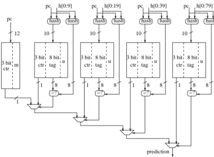
Predictor cbp1.5 is a global-history based predictor derived from PPM. PPM was originally introduced for text compression [1], and it was used in [2] for branch prediction. Figure 1 shows a synopsis of cbp1.5, which features 5 banks. It can be viewed as a 4th order approximation to PPM [3], while YAGS [4], which is a GPPM predictor too, can be viewed as a 1st order approximation. The leftmost bank on Figure 1 is a bimodal predictor [5]. We refer to this bank as bank 0. It has 4k entries, and is indexed with the 12 least significant
h[0:19] h[0:39] h[0:79] h[0:9]
=? hash hash
3 bit tag 8 bit
u
8 8
pc
hash
=? hash
ctr 10
pc
ctr 3 bit
tag 8 bit
u
8 8
10
hash
=? hash
ctr 3 bit
tag 8 bit
u
8 8
10
hash
=? hash pc
ctr 3 bit
tag 8 bit
u
8 8
10 pc
m ctr 3 bit
pc 12
prediction
1 1 1
1
1
Figure 1: Predictor cbp1.5 features 5 banks. The “bimodal” bank on the left has 4k entries, with 4 bits per entry. Each of the 4 other banks has 1k entries, with 12 bits per entry. The rightmost bank is the one using the most global history bits (80 bits).
bits of the branch PC. Each entry of bank 0 contains a 3-bit up-down saturating counter, and anmbit (mstands formeta-predictor) whose function is described in Section 2.3. Bank 0 uses a total of 4k×(3 + 1) = 16 Kbits of storage.
The 4 other banks are indexed both with the branch PC and some global history bits : banks 1,2,3 and 4 are indexed respectively with the 10,20,40 and 80 most recent bits in the 80-bit global history, as indicated on Figure 1. When the number of global history bits exceeds the number of index bits, the global history is “folded” by a bit-wise XOR of groups of consecutive history bits, then it is XORed with the branch PC as in a gshare predictor [5]. For example, bank 3 is indexed with 40 history bits, and the index may be implemented aspc[0 : 9]⊕h[0 : 9]⊕h[10 : 19]⊕h[20 : 29]⊕h[30 : 39] where ⊕denotes the bit-wise XOR. Section 2.4 describes precisely the index functions that are used in cbp1.5. Each of the banks 1 to 4 has 1k entries. Each entry contains an 8-bit tag, a 3-bit up-down saturating counter, and a u bit (u stands for “useful entry”, its function is described in Section 2.3), for a total of 12 bits per entry. So each of the banks 1 to 4 uses 1k×(3 + 8 + 1) = 12 Kbits.
The total storage used by the predictor is 16k+ 4×12k= 64 Kbits. 2.2 Obtaining a prediction
At prediction time, the 5 banks are accessed simultaneously. While accessing the banks, an 8-bit tag is computed for each bank 1 to 4. The hash function used to compute the 8-bit tag is different from the one used to index the bank, but it takes as input the same PC and global history bits.
Once the access is done, we obtain four 8-bit tags from banks 1 to 4, and 5 prediction bits from banks 0 to 4 (the prediction bit is the most significant bit of the 3-bit counter). We obtain a total of 4×8 + 5 = 37 bits. These 37 bits are then reduced to a 0/1 final prediction. The final prediction is the most significant bit of the 3-bit counter associated with the longest matching history. That is, if the computed tag on bank 4 matches the stored tag, we take the prediction from bank 4 as the final prediction. Otherwise, if the computed tag on bank 3 matches the stored tag, we take the prediction from bank 3. And so on. Eventually, if there is a tag mismatch on each bank 4 to 1, the final prediction is given by bank 0.
2.3 Predictor update
At update time (for instance at instruction retirement), we know the prediction, from which bankX ∈[0,4] it was obtained, and whether the prediction was correct or not.
Update 3-bit counter. We update the 3-bit counter on bankX, the one that provided the final prediction, and only that counter. This is the classical method [6] : the counter is incremented if the branch is taken, decremented otherwise, and it saturates at values 7 and 0. In general, people prefer to use 2-bit counters instead of 3-bit counters. However, in cbp1.5, 3-bit counters generate less mispredictions.
Allocate new entries. If X ≤ 3, and if the prediction was wrong, we allocate one or several entries in banks n > X (there is no need to allocate new entries if the prediction was correct). Actually, there was a tag miss on each bank n > X at prediction time. The allocation consists of “stealing” the corresponding entries by writing the computed tag for the current branch. This is done as follows. We read the 4−X u bits from banksX+ 1 to 4. If allubits are set, we chose a randomY ∈[X+ 1,4] and “steal” the entry only on bank
Y. Otherwise, if at least one among the 4−X u bits is reset, we “steal” only the entries which have their ubit reset.
As said previously, a “stolen” entry is reinitialized with the computed tag of the current branch. Moreover, the associated u bit is reset. Finally, the associated 3-bit counter is reinitialized either with value 3 (weakly not-taken) or 4 (weakly taken). This is done as follows. We read the m bit from bank 0. If m is set, we reinitialize the 3-bit counter according to the branch outcome, i.e., value 4 if the branch is taken, value 3 if the branch is not taken. Otherwise, if m is reset, we reinitialize the 3-bit counter according to the bimodal prediction from bank 0, i.e., value 3 if the bimodal prediction isnot-taken, value 4 if the bimodal prediction istaken.
Updating bitsuandm. If the final prediction was different from the bimodal prediction (which implies X >0), we update the u bit in bankX and the mbit in bank 0 as follows. If the final prediction was correct, bitsmanduare both set, otherwise they are both reset. The rationale is as follows. If the final prediction differs from the bimodal prediction, there are two situations :
• Bimodal is wrong. It means that the entry in bank X is a useful entry. By setting the u bit, we indicate that we would like to prevent this entry from being stolen by another branch. By setting the m bit, we indicate that the branch outcome exhibits
+ + h[20]
h[0] 20−bit history folded onto 8 bits
+ h[0] h[80] 80−bit history folded onto 10 bits
Figure 2: Global history folding can be implemented with a circular shift register (CSR) and a couple of XORs (symbol⊕).
correlation with the global history value, so new entries for that branch should be allocated by reinitializing the 3-bit counter according to the actual branch outcome. • Bimodal is correct. Prediction from bankX was wrong. This happens when a branch
exhibits randomness in its behavior, and its outcome is not correlated with the global history value (or the global history is not long enough). In that case, we are allocating many useless entries. Moreover, because allocation is done only upon mispredictions, it is safer to initialize 3-bit counters with the bimodal prediction, which represents the most likely branch outcome. So we reset them bit to mean this. Moreover, we reset theu bit to indicate that the entry has not been proven useful, so it can be stolen if another branch claims the entry.
2.4 Folded global history
A possible way to implement history folding would be to use a tree of XORs. For example, for the 40-bit history, h[0 : 9]⊕h[10 : 19]⊕h[20 : 29] ⊕h[30 : 39] requires a depth-2 tree (assuming 2-input XORs). For the 80-bit history, this requires a depth-3 tree. In practice, history folding can be implemented by taking advantage of the fact that we are not folding a random value, but a global history value derived from the previous history value [3]. Figure 2 shows two examples of how global history folding can be implemented with a circular shift register (CSR) and a couple of XORs. In cbp1.5, there is a 10-bit CSR in front of each bank 2 to 4 to compute the index. The index is then obtained by a bitwise XOR of the CSR bits with pc[9 : 0]⊕pc[19 : 10]. In front of bank 1, the index is simply
pc[9 : 0]⊕pc[19 : 10]⊕h[9 : 0]. History folding is also used for the tags. For each bank 1 to 4, we use a set of two CSRs, CSR1 and CSR2, which are respectively 8 bits and 7 bits. The tag is computed as pc[7 : 0]⊕CSR1⊕(CSR2 <<1). We used two CSRs because a single CSR is sensitive to periodic patterns in the global history, which is a frequent case.
3. Description of GPPM-ideal 3.1 Definitions
Our definition of GPPM-ideal is based on the notion of sequence frequency. We define the program control flow (PCF) as a finite sequence (Bi) of dynamic basic blocksBi ∈ Bwhere B is the set of all static basic blocks constituting the program text. We denote S(n) the set of all possible sequences of n consecutive blocks. In particular, S(1) = B. We denote
S(m, n) = Sk∈[m,n]S(k) the set of sequences whose length is between m and n. Given
m < n and two sequences u ∈S(m) ands∈S(n), we will say that u is a suffix of s, and denote itu≺s, if sequence umatches the last m blocks ofs.
For each sequence s, we define itsfrequency f(s) as the number of occurrences of s in the PCF. We assume that each block B ∈ B, hence each sequence, has only two possible successor blocks in the PCF, which is true for blocks ending on a conditional branch. We denote 1s and 0s the most frequent and least frequent successor block of sequence s in the PCF, respectively. By definition, ∀s∈ S(n), we have f(s.1s) ≥f(s.0s), where we denote
s.1s (resp. s.0s) the sequence from S(n+ 1) formed by appending block 1s (resp. 0s) to sequence s. The following example illustrates the definitions. Consider the short PCF below :
aababcdaaabcd
The set of blocks is B = S(1) = {a, b, c, d}. The set of two-block sequences is S(2) = {aa, ab, ba, bc, cd, da}. The frequency of sequence s=aa is f(s) = 3, and we have 1s =b, 0s = a,f(s.1s) = f(aab) = 2,f(s.0s) = f(aaa) = 1. Sequence bcd ∈ S(3) is a suffix of sequence babcd∈S(5), that is bcd≺babcd.
3.2 GPPM-ideal
The GPPM-ideal predictor consists of a setT of sequences. The number of sequences in T
is denoted |T|. Sequences in T have various lengths, which we assume are always strictly greater than one. We also assume that the content of T is fixed for the whole PCF. For eachBj in the PCF, we search for the longest sequences=Bj−n+1· · ·Bj inT, with n≥2. If we do not find such a sequence, the default sequence iss=Bj. Then the prediction from GPPM-ideal is 1s. If Bj+1 = 1s, this is a correct prediction; otherwise if Bj+1 = 0s we count a misprediction. The total number of mispredictions is
m(T) = X s∈S(1)
f(s.0s)−
X
s∈T
(f(s.0u)−f(s.0s)) (1)
whereuis the longest suffix ofsinB ∪T. Expression (1) can be understood as follows. All the potential mispredictions are counted in the sum Ps∈S(1)f(s.0s) +Ps∈Tf(s.0s). We must remove from this sum the “false” mispredictions on sequencesufor which there exists a longer matching sequence inT, i.e.,Ps∈Tf(s.0u). More explanations can be found in [7].
3.3 A heuristic for set T
We assume|T|is fixed. Our goal is to find aT that minimizesm(T). We defineS as the set of all sequences that are allowed to be in T. For example, if we allow all sequences whose length does not exceedN, we have S=S(2, N).
We defineS∗
⊆Sas the useful sequences remaining after removing fromSthe sequences
ssuch that 0s= 0u, whereu is the longest suffix ofsinB ∪S. It can be verified thatS∗ is the smallest subset of S such thatm(S) =m(S∗) =m(∅)−P
s∈S∗(f(s.1s)−f(s.0s)). We
order the sequences in S∗
according to the following procedure. Each sequence s∈S∗
has a potentialwhich we define as
f(s.1s)−f(s.0s) +
X
u∈S∗,s≺u
(f(u.1u)−f(u.0u))
We sort sequences inS∗in decreasing potentials, and we put inTthe first|T|sequences with
the highest potentials. This heuristic does not necessarily give an optimal set T. However in practice, it gives a curve m(T) as a function of |T|that is approximately convex, which ensures that we are close to an optimalT.
4. From GPPM-ideal to cbp1.5
All the results presented in this study are obtained with the CBP traces. To build GPPM-ideal, we first define a maximum sequence length N = 200, and we assume S ⊆ S(2, N). Each sequence from S that occurs in the PCF and that ends with a conditional branch is recorded in a table. For each sequence recorded, we maintain a count of the number of occurrences of the sequence in the PCF, and how many times the branch ending the sequence was taken. At the end of the PCF, we buildS∗ and sort sequences in decreasing potentials.
Then we compute m(T) from (1). Because of memory limitations on our machines, when |S|exceeded a certain size, we decreasedN. However, as the longest global history length in cbp1.5 is 80 branch direction bits, we did not want N to be smaller than 81. So we shortened a few traces, namely INT-2, INT-3, MM-1, MM-2 and MM-5.
4.1 Base results
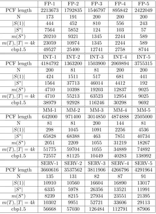
Table 1 gives the PCF length for each trace. We count in the PCF only the blocks ending on conditional branches, so the PCF length is in fact the number of dynamic conditional branches. The maximum sequence lengthN is indicated in Table 1 for each trace. |S(1)|is the number of unique static conditional branches encountered in the PCF. The set of allowed sequences isS=S(2, N). |S∗|is the number of useful sequences inS. A large value of|S∗|
means that GPPM predictors need a large global table. The number of mispredictions for GPPM-ideal for the given value of N, and with no size limitation, is m(S∗
). Table 1 also gives the value of m(T) when we constrain the global table size to not exceed |T|= 4096 sequences, where the content of T is determined as described in Section 3.3. Note that 4096 is also the number of global entries in cbp1.5. Finally, Table 1 shows the number of mispredictions for cbp1.5.
FP-1 FP-2 FP-3 FP-4 FP-5 PCF length 2213673 1792835 1546797 895842 2422049
N 173 191 200 200 200
|S(1)| 444 452 810 556 243
|S∗| 7564 5852 124 103 57
m(S∗
) 20210 9321 1345 2244 589
m(T),|T|= 4k 23059 10974 1345 2244 589 cbp1.5 49527 25400 12741 2758 8744
INT-1 INT-2 INT-3 INT-4 INT-5 PCF length 4184792 1363200 1503900 2069894 3755315
N 200 81 81 200 200
|S(1)| 424 1511 517 681 441
|S∗| 1564 37713 46014 4412 192 m(S∗) 4710 10398 19203 12837 9025 m(T),|T|= 4k 4710 55213 63523 12954 9025 cbp1.5 38979 92928 116246 30298 9692
MM-1 MM-2 MM-3 MM-4 MM-5
PCF length 642000 971400 3014850 4874888 2505000
N 81 81 200 144 81
|S(1)| 298 1045 1091 2256 4536
|S∗
| 65828 68388 463 7851 40734
m(S∗
) 2051 2209 1055 31219 18267
m(T),|T|= 4k 51775 59704 1055 34889 74892 cbp1.5 72557 81125 10449 40283 138992
SERV-1 SERV-2 SERV-3 SERV-4 SERV-5 PCF length 3660616 3537562 3811906 4266796 4291964
N 135 131 82 87 91
|S(1)| 10910 10560 16604 16890 13017 |S∗| 6335 5978 26356 13521 11991 m(S∗) 8239 8215 27934 23551 21395 m(T),|T|= 4k 10302 9951 52721 33606 29113 cbp1.5 56668 57030 126484 112791 87906
Table 1: Basic results for each trace. Traces INT-2,3 and MM-1,2,5 were shortened due to memory limitations, to keep N greater than 80.
step degradation
1 global history uses branch direction bits only 2 global history does not exceed 80 bits
3 allowed global history lengths are 10,20,40 and 80 bits
4 number of sequences of the same length cannot exceed|T|/4 = 1024 5 hash function and sequence allocation like cbp1.5, 30-bit tags 6 use 3-bit counters initialized with 1s
7 8-bit tags
8 initialize 3-bit counters using them bit 9 4k-entry direct-mapped bimodal
Table 2: Degradation path from GPPM-ideal to cbp1.5.
4.2 A degradation path from GPPM-ideal to cbp1.5
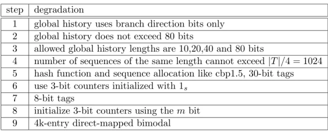
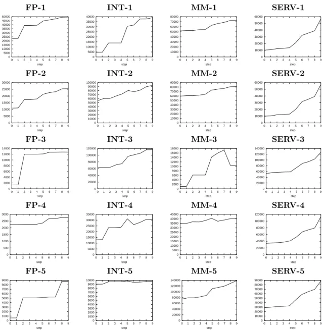
Table 2 gives an example of a degradation path from GPPM-ideal with|T|= 4096 to cbp1.5. We arbitrarily divided the degradation path into 9 steps, each step including the previous ones. Figure 3 shows the number of mispredictions after each step. Step 0 corresponds to GPPM-ideal, with S = S(2, N). GPPM-ideal is a path-based predictor, meaning that each sequence is identified with the PC of the conditional branch ending the sequence and with the PC of all the blocks constituting the sequence. However, cbp1.5 uses a global history of branch directions, which contains less information. Step 1 corresponds to the use of branch direction bits in the global history. As can be seen on Figure 3, the degradation is generally small, except for INT2, MM5, SERV3 and SERV4 (several thousands of extra mispredictions). Step 2 corresponds to not using more than 80 global history bits, i.e.,
S = S(2,81). It brings a significant degradation on FP traces, and on INT1, INT4 and MM3. Step 3 corresponds to limiting the allowed lengths toS =S(11)∪S(21)∪S(41)∪S(81). It is often a negligible degradation, but is significant on INT2, INT3, MM5 and SERV4. Step 4 splits T into 4 equally-sized partitions. That is, T cannot have more than |T|/4 = 1024 sequences with the same length. In each partition, sequences are sorted in decreasing potentials (Section 3.3). This mimics the 4 global banks in cbp1.5. The impact of step 4 is significant on INT2, INT3, SERV1, SERV2,and SERV4.
Step 5 is the biggest qualitative step. Starting at this step, the content of T is allowed to change dynamically. We can no longer use formula (1), and so now we generate results by performing a second pass on the traces. We use the 4 global banks of cbp1.5, and the same allocation policy as cbp1.5 i.e., the one based on the u bit. Moreover, we use 30-bit tags. However, the prediction for the longest matching sequence s is still given by 1s, as in GPPM-ideal. As expected, the magnitude of the degradation is strongly correlated with |S∗|. Step 6 corresponds to the introduction of 3-bit counters. Although predictions are now
given by 3-bit counters, the counter associated with sequences is initialized with 1s when we steal an entry fors. Except for a few cases (INT2, INT4, MM4), it increases the number of mispredictions. As expected, traces with a large|S(1)|, e.g. the SERV traces, experience a more pronounced degradation, corresponding to cold-start bimodal mispredictions. Step 7 corresponds to using 8-bit instead of 30-bit tags. This is a significant degradation on
FP-1 INT-1 MM-1 SERV-1 0 5000 10000 15000 20000 25000 30000 35000 40000 45000 50000
0 1 2 3 4 5 6 7 8 9 step 0 5000 10000 15000 20000 25000 30000 35000 40000
0 1 2 3 4 5 6 7 8 9 step 0 10000 20000 30000 40000 50000 60000 70000 80000
0 1 2 3 4 5 6 7 8 9 step 0 10000 20000 30000 40000 50000 60000
0 1 2 3 4 5 6 7 8 9 step
FP-2 INT-2 MM-2 SERV-2
0 5000 10000 15000 20000 25000 30000
0 1 2 3 4 5 6 7 8 9 step 0 10000 20000 30000 40000 50000 60000 70000 80000 90000 100000
0 1 2 3 4 5 6 7 8 9 step 0 10000 20000 30000 40000 50000 60000 70000 80000 90000
0 1 2 3 4 5 6 7 8 9 step 0 10000 20000 30000 40000 50000 60000
0 1 2 3 4 5 6 7 8 9 step
FP-3 INT-3 MM-3 SERV-3
0 2000 4000 6000 8000 10000 12000 14000
0 1 2 3 4 5 6 7 8 9 step 0 20000 40000 60000 80000 100000 120000
0 1 2 3 4 5 6 7 8 9 step 0 2000 4000 6000 8000 10000 12000 14000 16000 18000
0 1 2 3 4 5 6 7 8 9 step 0 20000 40000 60000 80000 100000 120000 140000
0 1 2 3 4 5 6 7 8 9 step
FP-4 INT-4 MM-4 SERV-4
0 500 1000 1500 2000 2500 3000
0 1 2 3 4 5 6 7 8 9 step 0 5000 10000 15000 20000 25000 30000 35000
0 1 2 3 4 5 6 7 8 9 step 0 5000 10000 15000 20000 25000 30000 35000 40000 45000
0 1 2 3 4 5 6 7 8 9 step 0 20000 40000 60000 80000 100000 120000
0 1 2 3 4 5 6 7 8 9 step
FP-5 INT-5 MM-5 SERV-5
0 1000 2000 3000 4000 5000 6000 7000 8000 9000
0 1 2 3 4 5 6 7 8 9 step 0 1000 2000 3000 4000 5000 6000 7000 8000 9000 10000
0 1 2 3 4 5 6 7 8 9 step 0 20000 40000 60000 80000 100000 120000 140000
0 1 2 3 4 5 6 7 8 9 step 0 10000 20000 30000 40000 50000 60000 70000 80000 90000
0 1 2 3 4 5 6 7 8 9 step
Table 3: Impact of the degradations listed on Table 2 on the number of mispredictions. Step 0 is GPPM-ideal, and step 9 is cbp1.5.
the INT and SERV traces. Step 8 corresponds to initializing 3-bit counters as in cbp1.5, that is, using information from the mbit instead of 1s. Except for MM3, this increases the number of mispredictions, and significantly for a majority of cases. Finally, the last step corresponds to limiting the bimodal table size. This is an important degradation for traces with a large |S(1)|, in particular the SERV traces.
5. Conclusion
The difference between GPPM-ideal and cbp1.5 cannot be attributed to a single cause. If we want to improve cbp1.5, we must work in several places. Steps 1 to 4 on Table 2 concern the choice of history lengths and the number and size of global banks. There is a potential for removing a significant number of mispredictions here, especially on the FP and INT traces. Step 5 is one of the biggest single contributors to the discrepancy between GPPM-ideal and cbp1.5. In cbp1.5, we steal an entry on each misprediction. A paradox of this method is that the more mispredictions we have, the more useful entries are replaced with useless ones. This is harmful positive feedback. We should find a better method than the u bit to decide which entry should be stolen and which should not, so we can eliminate this positive feedback. We should also find a better method than the m bit to initialize counters, since this method is the source of a significant number of extra mispredictions (step 8). Finally, the SERV traces require a large bimodal table. We should try to enlarge the bimodal table, or find a way to dynamically adjust the fraction of the overall predictor storage holding bimodal entries. Some of the CBP-1 predictors (e.g., [8, 9]) dynamically adjust the history lengths according to the application. This would be another way to achieve a similar goal.
Acknowledgements
The author wishes to thank Jared Stark for helping improve the english References
[1] J. Cleary and I. Witten, “Data compression using adaptive coding and partial string matching,”IEEE Transactions on Communications, vol. 32, pp. 396–402, Apr. 1984. [2] I.-C. Chen, J. Coffey, and T. Mudge, “Analysis of branch prediction via data
compres-sion,” in Proceedings of the 7th International Conference on Architectural Support for Programming Languages and Operating Systems, Oct. 1996.
[3] P. Michaud and A. Seznec, “A comprehensive study of dynamic global-history branch prediction,” Research report PI-1406, IRISA, June 2001.
[4] A. Eden and T. Mudge, “The YAGS branch prediction scheme,” in Proceedings of the 31st Annual International Symposium on Microarchitecture, 1998.
[5] S. McFarling, “Combining branch predictors,” TN 36, DEC WRL, June 1993.
[6] J. Smith, “A study of branch prediction strategies,” in Proceedings of the 8th Annual International Symposium on Computer Architecture, 1981.
[7] P. Michaud, “Analysis of a tag-based branch predictor,” Research report PI-1660, IRISA, Nov. 2004.
[8] A. Seznec, “The O-GEHL branch predictor.” 1st CBP, Dec. 2004.