Diphotons from Diaxions

(1)

Diphotons from Diaxions

THESIS

submitted in partial fulfillment of the requirements for the degree of

MASTER OF SCIENCE

in PHYSICS

Author : Anastasia Sokolenko

Student ID : s1576194

Supervisor : Alexey Boyarsky

2ndcorrector : Vadim Cheianov

(2)

(3)

Diphotons from Diaxions

Anastasia Sokolenko

Instituut-Lorentz, Leiden University 2300 RA Leiden, The Netherlands

May 31, 2016

Abstract

At the end of 2015 two collaborations ATLAS and CMS reported the diphoton excess at the invariant mass 750 GeV. In this work we consider the extension of the Standard Model where this peak can be explained. This model involves a heavy scalar particle and

a light scalar particle (axion) that come from the Peccei-Quinn symmetry breaking. Using different experimental data we find

the allowed parameter space of the model. We study the possibility to search for the light axion of this model at the intensity frontier experiments and show that, unfortunately, SHiP

and NA62 experiments will not be sensitive to the model. At the end we show that this model of 750 GeV excess can be falsified at

√

s=13 TeV LHC run. We make quantitative predictions for new

(4)

(5)

Chapter

1

The Standard Model

1.1 Introduction

The Standard Model of particle physics is a theory that combine three (electromagnetic, weak and strong) of four fundamental forces together. The pioneers in the development of this model was Glashow, Salam and Weinberg in the middle of sixtieth. During the next 30 years the model was

successfully tested. It was foundWandZbosons with the expected

prop-erties. Experimentally it was confirmed the existence of quarks. Then it was discovered the Higgs boson that increased confidence in the model.

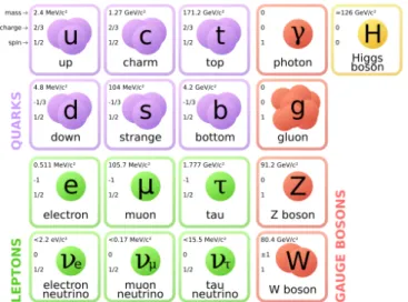
The Standard Model includes (Fig. 1.1) fermions, gauge bosons and the

Higgs boson. There are 12 elementary particles (antiparticles) with spin 1/2 called a fermions. This group involves six leptons (electron, electron neutrino, muon, muon neutrino, tau, tau neutrino) and six quarks (up, down, charm, strange, top, bottom). Quarks can not exist independently, in contrast to leptons. This phenomena is called color confinement. Thus quarks can not be observed as a free particle, they can be found only in some combination like mesons (quark and antiquark) and baryons (three quarks).

The word”quark” was appeared in the novel ”Finnegans Wake”, written

(10)

2 The Standard Model

The other particles, that have spin 1/2 are called leptons. From Greek the wordleptonmeans small, delicate or lightweight. At the beginning it was considered that leptons are ”light” particles comparing to hadrons (”heavy”). But in 1975 it was discovered the tau lepton and the word ”light” has lost its meaning.

Next let us go to bosons. All bosons have integer spin. The bosons play role in three of the four fundamental forces — electromagnetism, the strong force, and the weak force (gravity is not included in the standard model). These bosons are called gauge bosons. As we will see latter, each boson associated with some force: photon for electromagnetism, gluons for the strong force, and theWand Zbosons for the weak force.

In the standard model all particles are massless. The interaction that gives mass to elementary particles is called theHiggs mechanismand the particle that mediates the interaction is called theHiggs boson. The scalar field that is added to the Lagrangian to generate the masses to the fermions and vector bosons is theHiggs field.

Figure 1.1:The Standard Model of elementary particles.

The standard model is a successful model of elementary particles, how-ever it does not describe some phenomena such as dark matter, dark en-ergy, neutrino oscillations and baryogenesis.

2

(11)

1.2 Gauge Transformation

The symmetries play an important role in physics. As it happens, all in-teractions between the fundamental particles can be described using the principle oflocal gauge invariance. In this section we show an examples of local gauge invariance in the electrodynamics and in the electroweak part of the Standard Model .

1.2.1 Gauge invariance in the electrodynamics

Let us start from the free Dirac Lagrangian

LΨ =Ψ¯(i∂µγµ−m)Ψ. (1.1)

The Lagrangian is clearlynot invariantunder the local gauge transforma-tion

Ψ0 _→_e−iα(x)Ψ _(1.2)

because of the term∂µΨ.

Thus, we need to modify the partial derivative tosavethe invariance

∂µ →Dµ =∂µ−ieAµ, (1.3)

whereeis the charge of the electron and the vector field Aµtransforms in

the following way

A0_µ =Aµ+

1

e∂µα. (1.4)

The strength tensor is defined as

Fµν =

i

e[Dµ,Dν]. (1.5)

The main property of the strength tensor (1.5) is its invariance under the vector field transformation (1.4). In the abelian theory we can express the strength tensor in terms of the vector field Aµ as

Fµν =∂µAν−∂νAµ. (1.6)

The kinetic term can be construct from the strength tensors as

Lkin =−

1 4FµνF

(12)

This Lagrangian describes the free electromagnetic field.

Summing up, the gauge Lagrangian of the electrodynamics is

Lgauge =−1

4FµνF

µν₊Ψ¯₍_iD

µγµ−m)Ψ. (1.8)

This is an example of the abelian gauge theory.

It is needed to stress that the mass termm2AµAµ for the vector field is not

gauge invariant, so we can not add it to the gauge Lagrangian.

1.2.2 Electroweak gauge group of the Standard Model

Let us consider the electroweak group of the standard model

SU(2)L⊗U(1)Y . (1.9)

In the Standard Model there are two types of fermion fields: left and right. The right fermion field is a singlet and do not transform under SU(2)

transformation. The left fermion field is a doublet which transform under SU(2) transformation. The covariant derivatives for these left and right fermion fields are

DL →∂µ+i

g 2τ

i_Wi

µ−i

g0

2Bµ, (1.10)

DR →∂µ−ig0Bµ, (1.11)

where the gauge fields corresponding to each generator are

SU(2)L →Wµ1,W

2

µ,W

3

µ, (1.12)

U(1)Y → Bµ. (1.13)

The strength tensors for the gauge fields construct as in the case of the abelian theory (1.5). The results are

W_µνi _≡∂µWνi −∂νWµi +ge ijk_Wj

µW

k

ν, (1.14)

Bµν ≡∂µBν−∂νBµ, (1.15)

whereeijk is completely anti-symmetric tensor and gis the coupling

con-stant.

4

(13)

Now we are able to write the Lagrangian for the electroweak part of the Standard Model,

LEW =Ψ¯RiD/RΨR+Ψ¯LiD/LΨL−

1

4W

i

µνW

iµν₋1

4BµνB

µν _. _(1.16)

Let us notice that it is impossible to add mass terms to the fermion fields, as it should be in the formm(Ψ¯LΨR+Ψ¯RΨL), but the left fermion fieldΨL

is a doublet and the right fermion fieldΨRis a singlet. So its product is not

(14)

1.3 The Higgs Mechanism

In the previous section (1.2) we have seen that the mass terms arenot gauge invariantand that is why we are not allowed to add these terms to the

La-grangian. However, we know that some fundamental particles are

mas-sive. Thus, in this section we introducethe Higgs mechanism, which lets to add mass terms to the Lagrangian without explicit breaking of the gauge invariance. We start from the abelian Higgs mechanism as the simple ex-ample and than we consider how the Higgs mechanics works in the elec-troweak Standard Model.

1.3.1 The abelian Higgs mechanism

Let us consider the complex scalar Lagrangian

L=∂µφ∗∂µφ−V(φ∗φ), (1.17)

where the potential is

V(φ∗φ) = µ2φ∗φ+λ(φ∗φ)2, (1.18)

withλ>0.

It is needed to stress that the Lagrangian (1.17) is invariant under the global transformation

φ→ e−iθφ. (1.19)

We redefine the complex scalar field in terms of two real fields

φ= (φ1√+iφ2)

2 , (1.20)

and the Lagrangian (1.17) becomes

L = 1

2(∂µφ1∂

µ

φ1+∂µφ2∂µφ2)−V(φ1,φ2), (1.21)

which is invariant underSO(2)transformation.

The next step is to require a invariance under the local transformation

φ→eiqα(x)φ. (1.22)

6

(15)

To make the Lagrangian (1.17) invariant under the local transformation (1.22), we need to introduce a gauge bosonAµand the covariant derivative

Dµ

∂µ → Dµ =∂µ−ieAµ, (1.23)

Aµ → A0µ = Aµ+

1

e∂µα. (1.24)

We have two possible forms of the potential, depending on the sign of the parameterµ2.

• µ2>0

The vacuum is at

φ1 =φ2 =0. (1.25)

It means that we have two scalar fieldsφ1andφ2with massµ2.

• µ2<0

The vacuum is

q

φ2₁+φ₂2= −µ

2

2λ ≡

v2

2. (1.26)

The spontaneous symmetry breaking occurs forµ2<0. Indeed, when we

choose a particle vacuum, the SO(2)symmetry is spontaneously broken. Let us choose the vacuum in the following form

φ1 =v,

φ2 =0.

Introducing a small perturbations of the fieldsφ1andφ2

φ₁0 =φ1+v,

φ20 =φ2,

and the Lagrangian (1.17) becomes

L= 1

2∂µφ

0

1∂µφ10 +µ2φ012+ e2µ2

2

Aµ+

1 eµ∂

µ φ0₂

2

+ interaction terms.

(1.27) If we introduce new fieldBµ in the following way

Bµ = Aµ+

1 eµ∂

µ

φ02, (1.28)

than we see that this field Bµ is massive. As we can see, the field φ₁0 also

(16)

1.3.2 The non-abelian Higgs mechanism

From the experiment we know the masses of the gauge bosonsW and Z.

In this section we will show the origin of these masses and how it could derive from the scalar Lagrangian. Also we will show that the photon remain massless.

Let us start from the scalar Lagrangian

Lscalar =∂µΦ†∂µΦ−V(Φ†Φ), (1.29)

whereΦis the scalar doublet

Φ≡ φ+ φ0 . (1.30)

The potential is

V(Φ†Φ) = µ2Φ†Φ+λ(Φ†Φ)2, (1.31)

withλ>0.

We assume that the scalar Lagrangian should be invariant underSU(2)L⊗

U(1)Y. It means that we need to introduce the covariant derivative in the

following form

∂µ →Dµ =∂µ+ig τi

2W

i

µ+i

g0

2Bµ . (1.32)

We break the original symmetrySU(2)L⊗U(1)Y toU(1)EM choosing the

vacuum expectation value as

Φ0 =

0 v/√2

, (1.33)

where

v =

r

−µ2

λ . (1.34)

Substituting it into the scalar Lagrangian we get

Lscalar =

∂µ+ig τi

2W

i

µ+

ig0 2 Bµ

(v+H)

√ 2 0 1 2

−µ2(v+H)

2

2 −λ

(v+H)4

4 . (1.35)

8

(17)

Let us define the charged gauge bosons as

W_µ± = √1

2(W

1

µ∓iW

2

µ). (1.36)

From the Lagrangian (1.35) we get non diagonal mass terms for the fields W_µ3 and Bµ. Thus we need to diagonalize the mass matrix firstly. As a

result we obtain the physical fields Aµand Zµ

Aµ Zµ =

cosθW sinθW −sinθW cosθW

Bµ

W_µ3

, (1.37)

whereθW is the Weinberg angle is defined in terms of theSU(2)andU(1)

coupling constants

cosθW =

g p

g2₊_g02 , (1.38)

sinθW =

g0 p

g2₊_g02 . (1.39)

As we would like to get the Lagrangian in terms of the fields which we can observe experimentally, with the proper charge and mass, we need to rewrite the gauge fields for the generators in terms ofW_µν±,Aµ and Zµ.

These fields, as we will see later, are physical fields corresponding to W boson,Zboson and photon respectively.

One can rewrite the Lagrangian (1.35) it in terms of the fields W± and Z bosons and get the masses of these bosons.

Lscalar =     igW 1 µ

2 +g W_µ2

2

(v_√+H)

2

∂_√µH

2 −

igW

3

µ

2 −ig0 Bµ

2

(v_√+H)

2     2 −

−µ2(v+H)

2

2 −λ

(v+H)4

4 =

= 1

2H

2_M2 H +

1

2W

+

µW

−µ_M2 W+

1 2ZµZ

µ_M2

Z

+(∂µH)

2

2 +

µ4

4λ −H

3q

−µ2λ2−H4λ

4

+g

2

4 (2Hv+H

2₎

W_µ+W−µ₊ 1

2cos2_θ W

ZµZµ

(18)

where MH =

p

−2µ2, MA =0, MW = gv

2 and MZ =

gv 2 cosθW

.

As we can see the photon remains massless. The reason is that from the spontaneous symmetry breaking we obtain three Goldstone bosons, thus three gauge bosons get masses and one does not.

Finally, combining this result with the Standard Model gauge fields La-grangian (see appendix B), the structure of the SM LaLa-grangian for the scalar and gauge fields is

Lgauge+Lscalar =−

1 4FµνF

µν₋1

2W

+

µνW

−µν₋1

4ZµνZ

µν

+1

2H

2_M2 H +

1

2W

+

µW−

µ_M2

W+

1 2ZµZ

µ_M2

Z+

(∂µH)2

2

+ W+W−A + W+W−Z + W+W−ZZ + W+W−AA

+ W+W−ZA + W+W−W+W−

+ HHH + HHHH + W+W−HH

+ W+W−H + ZZHH + ZZH (1.40)

As one can see all parameters in the SM Lagrangian for gauge and scalar fields depends only on four constants —µ,g,g0andv. It is highly non

triv-ial prediction and it is entirely consistent with all available experimental data.

10

(19)

1.4 The Standard Model Phenomenology

1.4.1 Introduction

In this ”warm-up” section we will remind how to use the Lagrangian of

the Standard Model expressed in terms of physical fields γ, Z and W to

calculate physical observables. In sections 1.4.2 and 1.4.3 we will

calcu-late decay width ofWandZbosons and compare them with experimental

values. In section 1.4.4 we show how the mass of the Higgs boson can be constrained from the requirement of tree-level unitarity inW,W scat-tering. In section 1.4.5 we study decay channels of the Higgs boson in the Standard Model. This analysis of the SM phenomenology will be in-structive for the attempts to identify an extension of the SM that could be responsible for the reported access in di-photon signal. Although this signal still has to be confirmed, it provides and interesting possibility for Beyond Standard Model model building. This will be the main subject of the current thesis.

1.4.2 W

-boson decay width

W−_{, p}₁

e−, k2

ν, k1

Figure 1.2:Feynman diagram theWboson decay into a neutrino and an electron.

The matrix element for this process is

i_M =us1₍_k

2)√g

2γµ

1−γ5

2

vs2₍_k

1)eµ,r(p1). (1.41)

(20)

ele-12 The Standard Model

ment

|M|2= g

2

24Tr

"

γµ(1−γ5)/k1γν(1−γ5)(/k2−Me) −gµν+

pµ₁pν

1 M_W2

!#

=

= g

2

24M_W2 Tr[γµ(1−γ5)/k1γν(1−γ5)(/k2−Me)p

µ

1p

ν

2]

− g2

24Tr[g

µν

γµ(1−γ5)/k1γν(1−γ5)(/k2−Me)] =

= g

2

24{16(k1·k2) +8/M

2

W[2(k1·p)(k2· p)−(k1·k2)p21]} =

g2M2_W 3

The decay width for the process when a particle of mass Mdecays into 2

particles of massesm1andm2, is given by

dΓ = 1

32π2|M|

2|k1|

M2dΩ, (1.42)

where _|k1| = [(M2−(m1+m2)2)(M2−(m1−m2)2)]1/2/2M and dΩ is

the solid angle. In our case it leads to

ΓW_→νe =

g2MW

48π . (1.43)

Computing the decay width, we obtain the value ΓW_→νe = 0.227 GeV.

Due this channel theW boson decay with 10.75% probability [16], so the

full decay width is equal to Γtheory_W = 2.112 GeV. Our result is consistent with the experimental valueΓ_Wexp =2.085±0.042 GeV.

1.4.3 Z

-boson decay width

Without any difficulties, one can find the matrix element

iM =us1₍_p

1)

− ig

2 cosθW

γµ(vf −afγ5)

vs2₍_p

2)eµ,r(k), (1.44)

The axial and the vector couplingaf andvf defined as,

vf =T3−2Qsin2θW , (1.45)

12

(21)

Z, k

f, p1

f , p2

Figure 1.3: Feynman diagram for theZboson decay into a fermion and an anti-fermion pair.

af = T3, (1.46)

whereQ =T3+1₂Yis the hypercharge.

The square of the matrix element, where we again average over the spins and polarizations of the final state and neglect the mass of the fermion,

|M|2 = −g

2

12 cos2_θ WTr

[γµ(vf −afγ5)(/p₂−Mf)γµ(vf−afγ5)(/p₁−Mf)] =

= 8g

2

12 cos2_θ W

(a2_f +v2_f)(p1·p2) = g 2

3 cos2_θ W

(a2_f +v2_f)M2_Z.

Thus the decay width for the processZ → f f is given by

Γ_Z_→_{f f} = g

2

48π cos2θW

MZ(a2f +v2f) . (1.47)

The value of the constantsaf andvf for the different fermion flavors are

f f pairs af vf

ee,µµ,ττ -1/2 -0.06

uu,cc 1/2 0.21

dd,ss,bb -1/2 -0.35

νeνe,νµνµ,ντντ 1/2 1/2

(22)

f f pairs Decay width(theory), GeV Decay width(experimental [16]), GeV

ee,µµ,ττ 0.086 0.084

uu,cc 0.30 0.29

dd,ss,bb 0.38 0.39

νeνe,νµνµ,ντντ 0.170 0.167

We see that our theoretical predictions are in good agreement with the data. Comparing theoretical predictions and experimental values we can constrain many possibilities to extend the SM. For example, we can con-clude that there are no more SM-like generations of fermions. Indeed, if a fourth generation existed, than the decay width would be large then in the real world. The same we can say about the three colors of quarks, the theory is consistent with the experimental date only for three colors of quarks.

1.4.4 Bounds on the Higgs boson mass

The existence of the Higgs boson is necessary for the consistency of the Standard Model. Namely, from the requirement of tree-level unitarity one can obtain an upper bounds on the Higgs boson mass. Bellow we demon-strate this analyzingWW scattering at tree level.

Using the Goldstone Boson Equivalence Theorem [19], which states that at

high energies the amplitude M for emission or absorption of a

longitu-dinally polarized gauge boson is equal to the amplitude for emission or absorption of the corresponding Goldstone boson,

M(W_L±,Z_L0) ≈ M(ω±,z0) +O(M2_W_,_Z/E2). (1.48)

The scalar Lagrangian

Lscalar =∂µΦ†∂µΦ−V(Φ†Φ) (1.49)

can be rewritten if we express the Higgs doublet in terms ofω±andz0,

Φ = √1

2

i√2ω+

v+H₋iz0

. (1.50)

14

(23)

Thus the scalar Lagrangian in terms ofω±andz0is

Lscalar =∂µω−∂µω++

1 2∂µH∂

µ_H₊1

2∂µz

0

∂µz0− −µ21

2[2ω

−_ω+_{+ (}_v₊_H₎2_{+ (}_z0₎2_]

−λ1

4[4(ω

−_ω+₎2_{+ (}_v₊_H₎4_{+ (}_z0₎4₄

ω−ω+(v+H)2+

+4ω−ω+(z0)2+2(v+H)2(z0)2] =

=∂µω−∂µω++

1 2∂µH∂

µ_H₊1

2∂µz

0

∂µz0

−1

2H

2_M2 H−

M2_Hg 4MW

H[H2+2ω+ω−+ (z0)2]− − g

2_M2 H

32M_W2 [H 2₊₂

ω+ω−+ (z0)2]2

The structure of this Lagrangian shows immediately all needed interaction and vertices,

Lscalar =∂µω−∂µω++

1 2∂µH∂

µ_H₊1

2∂µz

0

∂µz0

−1

2H

2_M2 H−

M2_Hg 4MW

HHH +2 Hω+ω− + Hz0z0

− g

2_M2 H

32M_W2

HHHH +4ω+ω−ω+ω− + z0z0z0z0

+4 HHω+ω− +2 HHz0z0 +4z0z0ω+ω−

.

Now we are ready to compute the scatteringω+ω− → ω+ω−. There are

(24)

•

ω+_{, k} 1

ω−, k2

ω−_{, p}₁

ω−, p2

Figure 1.4:Feynman diagram for theωωscattering.

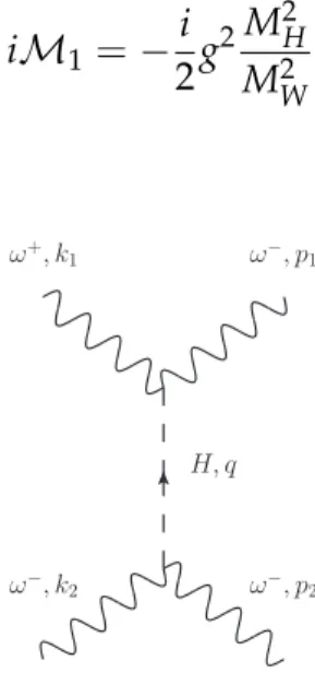
The matrix element is

iM1=−i

2g

2M2H

M_W2 . (1.51)

•

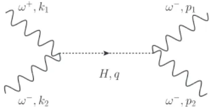
ω+_{, k} 1

ω−_{, k}

2

ω−_{, p}₁

ω−_{, p}

2

H, q

Figure 1.5:Feynman diagram for theωωscattering via the Higgs boson.

iM2 = −i

2g

2M2H

M2_W !2

i

(k1−p1)2−M2_H

. (1.52)

16

(25)

•

ω+_{, k} 1

ω−_{, k}₂

ω−_{, p}₁

ω−_{, p}₂ H, q

Figure 1.6:Feynman diagram for theωωscattering via the Higgs boson.

iM3 = −i

2g

2M2H

M2_W !2

i

(k1+k2)2−M2H

. (1.53)

Therefore the total matrix element is the sum of these three processes,

i_M=₋i

2g

2M2H

M2_W+ − i 2g

2M2H

M2_W !2

i

(k1−p1)2−M2_H

+ i

(k1+k2)2−M2_H !

.

(1.54) Introducing the Mandelstam variables, which are defined by

s = (k1+k2)2 =2k1k2, (1.55)

t = (k1−p1)2=−2k1p1, (1.56)

the matrix element could be present as,

iM=−ig

2_M2 H

4M2 W

2+ M

2 H

s₋M2 H

+ M

2 H

t₋M2 H

!

. (1.57)

At the high energies limit we obtain the following expression for the am-plitudeM(W_L±,Z_L0) ≈ M(ω±,z0)

|M|=

g2M2_H 2M_W2

. (1.58)

Unitarity requires, that the amplitude shoul be less than some constant,

|M| < 16π. From this restriction we get the upper limit on the Higgs

mass,

4√2π

GF

> M2_H . (1.59)

(26)

1.4.5 The decay modes of the Higgs boson

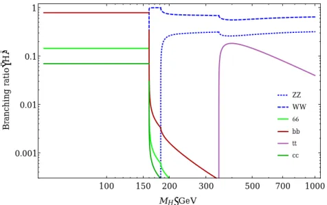
Here we will compute the Higgs branching ratios, depending on the Higgs mass, by considering the tree level diagrams for the possible decay modes of the Higgs boson. At the tree level the Higgs boson interacts only with a

fermions,W± andZbosons.

• H → f f

H, q

f , k1

f, k2

Figure 1.7:Feynman diagram for the Higgs boson decay into a fermion and anti-fermion pair.

i_M1=v(k2)

−_igM

f

2MW

u(k1), (1.60)

and the square of the matrix element is

|M1|2 = g2M2_f

4M2_WTr[(/k1−Mf)(/k2−Mf)] =

= g

2_M2 f

4M_W2 4(k1·k2) = g2M2_f

2M2_W(M 2

H +2M2f). (1.61)

Here we are not able to neglect the mass of the fermion! So the decay width is given by

Γ= g

2_M2 f

32πMHM_W2

(M2_H +2M2_f)

s

1₋

₂_M f

MH 2

. (1.62)

If the Higgs boson is heavy enough, so it is possible to decay into theW±

andZbosons,

18

(27)

• H →W+W−

H, q

W+_{, k} 1

W−, k2

Figure 1.8: Feynman diagram for the Higgs boson decay into the W+ and W− bosons.

The matrix element and the square of the matrix element are,

i_M2 =eµ(k1)eν(k2)igMWgµν, (1.63)

|M2|2 =g2M2W 2+

(M2_H −2M2_W)2

4M4_W

!

. (1.64)

Thus, the decay width is

Γ = g

2_M2 W

16πMH 2+

(M2_H−2M_W2 )2

4M4 W

! s

1−

2MW

MH 2

. (1.65)

• H → Z0Z0

H, q

Z, k1

Z, k2

Figure 1.9:Feynman diagram for the Higgs boson decay into twoZbosons.

The only difference of this process withH _→W+W− is the coupling con-stant, so

i_M3=eµ(k1)eν(k2) ig cosθW

MZgµν, (1.66)

|M3|2 =

g2M2_Z cos2_θ

W

2+(M

2

H −2M2Z)2

4M4_Z

!

(28)

with the decay width

Γ = g

2_M2 Z

32πMHcos2θW

2+(M

2

H −2M2Z)2

4M4_Z

! s

1₋

2MW

MH 2

. (1.68)

Let us demonstrate these results graphically, depending on the Higgs bo-son mass for the different gauge bobo-sons and fermion flavors.

ZZ WW ΤΤ bb tt cc

100 150 200 300 500 700 1000

0.001 0.01 0.1 1

MH@GeVD

Branching

ratio

H

L

Figure 1.10:Predicted branching ratio of the Higgs boson at the tree level.

20

(29)

The precise calculation leads to the following dependence [20],

Figure 1.11: Predicted branching ratio of the Higgs boson including loop contri-butions.

The vivid differences between our calculations (Fig. 1.10) and the precise calculations with taking into account the loop contributions (Fig. 1.11) are the following:

1. The behavior of the curves forZZ andWW in the Higgses mass

re-gion between 100 and 200 GeV. It is because of the fact that our cal-culation consider thatZandW should be real particles. Thus in our calculations the Higgs with the mass lower that about 200 GeV can not decay into these bosons, while in reality it can via virtualZand

Wbosons.

2. The presence of the decay channels into γγ and γZ. In the SM

La-grangian there not exist the vertices like Hγγ and HZγ. So at the

(30)

(31)

Chapter

2

Diphoton excess at the LHC

2.1 Overview of the Diphoton Excess

At the end of 2015 year two collaborations ATLAS [10] and CMS [9] re-ported the excess in the diphoton resonance. From the data of proton-proton collisions at the LHC at the center-of-mass energy√s = 13 TeV it was observed an diphoton excess near the invariant mass 750 GeV. One of the explanation of this signal is a new particle with spin zero or two (spin 1 is forbidden because ofthe Landau-Yang theorem). This signalhas notbeen confirmed as we do not have enough data.

Both experiments, ATLAS and CMS, were present the diphoton excess at the center-mass-energy√s =13 TeV.

The ATLAS collaboration reports the following numbers of events (see table 2.1) in the interested region with the luminosity L = 3.2 fb−1 (see appendix E) and the SM background. The local significance at the dipho-ton invariant mass∼ 750 GeV is 3.9σ and the global significance is 2.3σ.

Thelocal significancemeans the deviation from the expectation divided by

the standard deviation in the region of the resonance peak. The global

significance considers the Look Elsewhere Effect, i.e. with taking into ac-count a probability of accidental fluctuations in the hole region of mea-surements.

Bin, GeV 650 690 730 770 810 850

Nevents 10 10 14 9 5 2

(32)

24 Diphoton excess at the LHC

[GeV]

γ γ

m 200 400 600 800 1000 1200 1400 1600

Events / 40 GeV

1 − 10 1 10 2 10 3 10 4 10 ATLAS Preliminary -1

= 13 TeV, 3.2 fb s Data Background-only fit [GeV] γ γ m 200 400 600 800 1000 1200 1400 1600 Data - fitted background −15

10 − 5 − 0 5 10 15

Figure 2.1:Invariant mass distribution of the selected diphoton events at ATLAS detector.

With regards to CMS collaboration, they reported the results with 2.6 fb−1 for two distinct categories. In the first one both photons are detected in the barrel (EBEB) and in the second one the first photon is detected in the barrel and the other one is found in the end cap (EBEE). The numbers of events in the interested region at the diphoton invariant mass around 750 GeV with the local significance 2.6σ and with the global significance

2σ, for both categories in presented below.

Bin, GeV 700 720 740 760 780 800

Nevents(EBEB) 3 3 4 5 1 1

Nbackground(EBEB) 2.7 2.5 2.1 1.9 1.6 1.5

Nevents(EBEE) 16 4 1 6 2 3

Nbackground(EBEE) 5.2 4.6 4.0 3.5 3.1 2.8

From the experimental data it is complicated to determine the resonance decay width. The data from the ATLAS collaboration indicates the wide decay width, while the CMS collaboration data favors the narrow decay

24

(33)

2.1 Overview of the Diphoton Excess 25

Events / ( 20 GeV )

-1 10 1 10 2 10 Data Fit model σ 1 ± σ 2 ± -2 10 ⋅ 2 × γ γ → ) =0.01 κ∼ G( EBEE category (GeV) γ γ m 2 10 ×

3 ₄_×₁₀2 ₅_×₁₀2 ₁₀3 ₂_×₁₀3

stat σ (data-fit)/ -4 -2 0 2 4 (13 TeV) -1 2.6 fb CMS Preliminary

Figure 2.2:Observed invariant mass spectrum for the EBEB at CMS detector.

Events / ( 20 GeV )

-1 10 1 10 2 10 Data Fit model σ 1 ± σ 2 ± -2 10 ⋅ 2 × γ γ → ) =0.01 κ∼ G( EBEB category (GeV) γ γ m 2 10 ×

3 ₄_×₁₀2 ₅_×₁₀2 ₁₀3 ₂_×₁₀3

stat σ (data-fit)/ -4 -2 0 2 4 (13 TeV) -1 2.6 fb CMS Preliminary

Figure 2.3:Observed invariant mass spectrum for the EBEE at CMS detector.

width. In this work we assume the wide decay width

Γ=40 GeV . (2.1)

The experimental cross-section is defined as (see appendix D and E)

σ(pp →s) = BR×N(pp→s)/L, (2.2)

whereN(pp →s)is the number of events,Lis a luminosity andBRis the branching ratio.

In the paper [7] was analyzed the data for ATLAS (√s = 8 TeV with

(34)

19.7 fb−1 and √s = 13 TeV with 2.6 fb−1), and to be consistent with the data we have some constraints for the ratio of the cross sections at differ-ent energies:

σ(pp →γγ) ≈      

    

(0.5_±0.6)fb CMS[11] √s =8TeV,

(0.4±0.8)fb ATLAS[12] √s=8TeV,

(6_±3)fb CMS[9] √s =13TeV,

(10±3)fb ATLAS[10] √s=13TeV.

The data from 8 to 13 TeV are satisfy to each other at 2σ if the gain

fac-tor

r =σ13TeV/σ8TeVat least more than 5 [8] (2.3)

Combining four data sets (see table 2.1) and assuming the invariant mass 750 GeV and the decay width 40 GeV, one can get the best fit for the cross

section for the diphoton resonance at the invariant mass energy√s = 13

TeV,

σ(pp →s)×BR(s →γγ)∼6 fb . (2.4)

Thus, while we are waiting for new data to justify or falsify the diphoton excess, knowing some parameters, such as the number of events, the decay width and the cross section, we are able to construct a theory which may describe the resonance.

26

(35)

2.2 A Simple Model

The toy model which could describe such resonance involves some heavy scalar partial s with spin zero, decays into two photons [8]. The natural question is: How this particle was produced? As we will see letter this

par-ticlecan not produced only from photons. Indeed, if s is produced from

photons, we can calculate the cross section of s production, scales with the energy. From this calculation, one can conclude that in this case a

simi-lar diphoton signal would beobservedalready at LCH run at 8 TeV! But

we did not find any signal above the background. Thus we assume that the heavy scalar particle produced from gluons. In the end of this

chap-ter it will shown that the theory with only the gluons and photons also

contradict with the experimental data.

The corresponding Lagrangian is

L=LSM+Lint+Lkin, (2.5)

whereLSMis the Lagrangian of the SM,Lint is the interaction Lagrangian

of the new scalar particle with gluons and photons, and _Lkin its kinetic

Lagrangian.

In the next chapters we redefineLint asLfor the convenience.

Thus,

L= cgαs

12π

s

ΛGµνGµν+

2α

9πcF

s

ΛFµνFµν , (2.6)

where cg and cF are the coupling constants, α and αs are the electroweak

force and the strong force coupling constants,Λis some energy scale of a new physics, which shows when our theory stops work.

The strength tensors for the gauge fields are

Gµν ≡∂µGν−∂νGµ+cg[Gµ,Gν], (2.7)

Fµν ≡∂µFν−∂νFµ. (2.8)

The cross section for A+B _→ R_→ C+D[15] scattering process is given

by

σ(s) =32π 2JR+1

(2JA+1)(2JB+1)

ΓABΓCD

(s−m2_{) +}_m2Γ2 , (2.9)

(36)

We are interested in the proton-proton collisions with two photons in the final state (Fig. 2.4). The cross-sectionσαα→s→γγ is described by formula

(2.9), whereαis a type of the particle (in our case a gluon or photon).

s

γ

p p

α α

Figure 2.4: Production of the heavy scalar particle from the proton-proton colli-sion viaαfusion.

To find out the full cross-section σpp→αα→s→γγ we need to use the

Par-ton Distribution Functions fα(x) (PDFs), where x is a Bjorken variable that

shows a fraction of proton’s momentum carried by the particle. With the PDFs we are able to calculate the full cross-section by the formula

σpp→αα→s→γγ(s) =

∑

α=g,γ

1

Z

0

dx1fα(x1) 1

Z

0

dx2fα(x2)σαα→s→γγ(sαα). (2.10)

In the laboratory frame the particleαhas the momentums

p1 = (x1√s/2, 0, 0, x1√s/2)and p2= (x2√s/2, 0, 0, −x2√s/2).

Using the formula sαα = (p1 + p2)2 we find out relation between sαα

ands

sαα=x1x2s. (2.11)

We have the final result for the cross section

σpp→αα→s→γγ(s) =

∑

α=g,γ

1

Z

0

dx1fα(x1)×

×

1

Z

0

dx2fα(x2)

32π

(2Jα+1)2

ΓγγΓαα

(x1x2s−m2)2+m2Γ2

, (2.12)

whereΓ=Γgg+Γγγ =40 GeV (2.1).

28

(37)

To simplify this, let us use the delta-function approximation for the narrow

width, which is valid formΓ(see appendix C),

dx

(x₋m2₎2₊_m2_Γ2 mΓ

π →δ(x−m

2₎_dx_, _(2.13)

and we get the following expression

σpp→s→γγ(s) =

∑

α=g,γ

1

Z

m2_/_s

dx fα(x)

32π

xs

π

mΓfα

m2 sx

1

(2Jα+1)2

ΓγγΓαα.

Rewriting the cross section in terms of the dimensionless partonic integrals we get,

σpp→s→γγ(s) = Γγγ

mΓs_α₌

∑

_g_,_γCααΓαα, (2.14)

where the partonic integrals are

Cgg = π 2

8

1

Z

m2_/_s

dx

x fg(x)fg

m2 sx

, (2.15)

Cγγ =8π2

1

Z

m2_/_s

dx

x fγ(x)fγ

m2 sx

. (2.16)

The numerical values [8] of the partonic integrals are the following, √

s,TeV Cgg Cγγ

8 174 11

13 2137 54

In particular, from the equation (2.14) one can find the value of the gain factors (2.3) for the gluon and photon fusions as

rαα =σ13 TeV(pp →αα →s→γγ)/σ8 TeV(pp →αα →s→γγ),

Thus the gain factors for the gluon and photon fusions are

(38)

As we mentioned above (2.3), to satisfy the experimental data we need r/5 ∼1. It means thatsproduces mainlyvia gluon fusion.

Using the equation for the cross section (2.14) and the fact that the new

heavy scalar particle with mass ∼ 750 GeV produces mainly via gluon

fusion with the cross-section σpp→s→γγ = 6 fb (2.4), we can find out Γgg

andΓγγfrom the following system of equations

  

 

Γγγ

m

Γgg

m ≈1.2×10

−6Γ

m ≈7.1×10

−8_,

Γ

m =

Γgg

m +

Γγγ

m ≈0.06.

We find two solutions:

1. Γgg/m=5.3×10−2andΓγγ/m =1.3×10−6,

2. Γgg/m=1.3_×10−6andΓγγ/m =5.3×10−2.

We chose the first one as we know, from the gain factor argument, that the production from the photon fusion should be suppressed.

Thus,

Γgg/m=5.3×10−2and Γγγ/m =1.3×10−6. (2.18)

Next we will show why this solution can not be satisfactorily. From the experiment [13] we have the constraint on the value of Γgg. It can notbe too large, as the processgg_→s _→ggispossible. If we want to produce the new scalar particle from the gluons, we need to take into account that it

de-cays mainly into two gluons! Based on the data from CMS at√s =8 TeV

we can find out the upper limit on the gluon-gluon production. From the plot 2.5 at the energy 750 GeV we get the cross section

σ×BR(X → jj) ≤1.8pb, (2.19)

and from the formula (2.14) we find the upper limit onΓgg/m

Γgg

m =

s

σ×BR(X →jj)Γs

mcgg ≤2.7×10

−3_. _(2.20)

Itcontradictsour theoretical prediction (2.18).

The decay width istoo big. Too big means that the heavy scalar particle s should interacts strongly with photons and gluons. Thus we reached the

30

(39)

conclusion that this big decay width not because of gluons! So to try to explain the resonance, we probe the simple model that involves only new heavy scalar particle and the SM particles. But we convinced ourself that any SM particlescan notsolve the problem with large decay width.

One way to solve this problem is to add a new light scalar particle, as one can see in the next chapter.

Resonance Mass [GeV]

600 800 1000 1200

A [pb]

×

jj)

→

BR(X

×

σ

2

−

10

1

−

10 1 10

2

10

3

10

95 % CL Upper Limit

Gluon-Gluon

Quark-Gluon

Quark-Quark

| < 1.3

η ∆

| < 2.5 & |

η

|

(8 TeV) -1 18.8 fb

CMSPreliminaryData

(40)

2.3 Diphotons from Diaxions

In this section we will consider the simple extension of the SM [2]. We add some non-SM particle in the simple theory (2.2) in such way, that this large decay widthis because of thisnew particle. In this case weavoidthe contradiction with the experimental data that we have had before. We cal-culate the productions and decays of the new particles (see sections (2.4) and (2.5)). Than we test this theory and find the constraints on the param-eters (see section (2.6)) by using the different experimental data.

Despite the fact that in the literature [2] it was discussed that the axion can be searched at SHiP and NA62 experiments, we will show that it is impossible.

The so-calledaxion-like particle (ALP) arises from the spontaneously

sym-metry breaking of a globalU(1) Peccei-Quinn (PQ) symmetry by a

com-plex fieldφ

φ= f√+s

2 e

ia

f _. _(2.21)

where f is the energy scale.

We expect themassiveparticlesandmasslessparticlea(the Goldstone bo-son), which comes from the Peccei-Quinn symmetry. If the Peccei-Quinn symmetry isslightlybroken, the axion becomesmassive, but much lighter that the heavy scalar particles.

The Lagrangian for the generic interactions for the diphoton resonance is

L= cgαss

12πfGµνG

µν₊3αcγa

4πf e

αβγδ_F

αβFγδ+s

(∂µa)2

f , (2.22)

where like in the simple model,cgandcFare the coupling constants,αand αs are the electroweak force and the strong force coupling constants, f is

some scale constant with the dimension of the energy.

The first term in the Lagrangian (2.22) is the same as in the simple model (2.6). The second term expresses how axions interacts with the photons. The anti-symmetric tensor eαβγδ shows that a is the pseudo-field, which

means that in the mirror it is not the same. The last term in the Lagrangian comes from the kinetic term of the fieldφ. That is why it does not have

coupling constants.

32

(41)

2.3 Diphotons from Diaxions 33

p

s

a

γ

γ γ

γ α

α

Figure 2.6: Production of the heavy scalar particle from the proton collision and its decay into two axions.

Thus in our model a heavy scalar particle s decays into two axions and

each axion decays into two photons (Fig. (2.6)). At the end we get four

photons, but we detectonly two photons!How does it agree with the experi-mental data? To solve this contradiction we assume that the axion-like par-ticle isvery lightandvery relativisticand photons from its decay arehighly collimated! Indeed, when the heavy scalar particlesdecay into two very light particles, each of them would have a large kinetic energy. And when the light particle with a great kinetic energy decays into massless photons, they are highly collimated, and the detector isunableto distinguish these

two photons from one photon. Thus we detect two photons, not four

pho-tons.

So, we avoid the contradiction with the experimental data that we had before, assuming that the large decay width is because of the axions. Now

we have the theory that describes the resonance. How to check that this

description is correct?

First of all let us derive the Feynman rules for this theory. From the La-grangian (2.22) we are able to conclude that a heavy scalar particles inter-acts with gluons and the light scalar particles a, the light scalar particles interacts withsand photons. Thus we get the vertices

a, k1

a, k2

s, p

= −2i f k

µ

1kν2gµν

(42)

g, k1

g, k2

s, p µ

ν

= icgαs 3πf [(k

µ

2·kν1)−gµν(k1·k2)]

Figure 2.8:The vertex forggs

ν µ

γ, k2

γ, k1

a, p

= −6iαcγ

πf e

αµβν_k

1αk2β

Figure 2.9:The vertex forγγs

34

(43)

2.4 Production of the Heavy Scalar Particle

The heavy scalar particlescan produced via thegluon production, photon fu-sionsand also via theassociated productionof the photons. Using the Feyn-man rules for this theory (2.22), which we derive in the previous section, we are able to calculate the cross sections for the s production at the tree level.

2.4.1 The production of the heavy scalar particle via the

gluon fusion

g, k1

g, k2

s, p µ

ν

Figure 2.10:Production ofsvia gluon fusion

The matrix element consequently is

i_M=icgαs

3πf[gµν(k1·k2)−(k2µ·k1ν)]e µ₍_k

1)eν(k2). (2.23)

The square of the matrix element is

|M|2 = c

2 gα2s

9π2f2[gµν(k1·k2)−(k2µ·k1ν)]e µ₍_k

1)eν(k2)×

×[gγδ(k1·k2)−(k2γ·k1δ)]eγ(k1)eδ(k2). (2.24)

Averaging over the polarizations of the initial state and taking into account that we have 8 types of the gluons one can get

|M|2 ₌ c 2 gα2s

144π2f2(k1·k2)

2 ₌ c 2 gα2sM4s

576π2f2. (2.25)

The differential cross-section (see appendix D) is given by

dσ(sgg) = (2π) 4

4

|M|2 p

(k1·k2)2

(44)

wheredΦ(k1+k2,p) =δ4(k1+k2−p) d 3_p

(2π)32Es.

Thus the cross section is

σ(sgg) = π|M| 2

2M3 s

δ(√sgg−Ms) = π|M| 2

2M3 s

2Msδ(sgg−Ms2) =

= π

576

cgαsMs

πf 2

δ(sgg−Ms2), (2.27)

and the full cross section can be find as in the case of (2.10),

σpp→s(s) = 1

Z

0

dx1f(x1) 1

Z

0

dx2f(x2)σ(sgg) =

Cgg

72πs

cgαsMs

πf 2

. (2.28)

Thus the cross section for the gluon fusion at√s=13 TeV is

σpp→s =107 fbc2g

320 GeV f

2

. (2.29)

The gain factorris,

rgg =σ13 TeV/σ8 TeV =4.7 . (2.30)

2.4.2 The production of the heavy scalar particle with jets

in the final state

In QCD there are a lot of ways to get jets in the final state in the proton-proton collision.

First of all let us consider one jet and s in the final state. There are 19 different processes with 22 diagrams (we do not distinguish the type of gluons and the color of quarks): gg_→ gs,qq¯ _→ gs,qg _→ qsand ¯qg _→qs¯ , some diagrams of these processes are presented on Figure 2.11.

For two jets and the heavy scalar particle in the final state we have 133 different processes with 344 diagrams.

For three jets and the heavy scalar particle we get 205 different processes with 4526 diagrams.

36

(45)

2.4 Production of the Heavy Scalar Particle 37 g g g s (a) g g g s g (b) g g s g (c) q ¯ q g g s (d) g q q g s (e) g ¯

q q¯

g s

(f)

Figure 2.11: Feynman diagrams of the production of the heavy scalar particle with one jet in the final state.

However, the logic of perturbation theory tells us that the contributions of the processes with many out coming jets should be suppressed. Only soft (low energy) multiple jets can contribute significantly, dues to strong coupling of QCD in the infra red. Therefore in our perturbative calcu-lations we have to take into account only the jets with large pt and the

non-perturbative soft jets contributions are already effectively encoded in the PDFs. To take this into account we will calculate this diagrams using

the packageMadGraph 5.

At the beginning let us find out the parametric dependence of all these processes. Regardless how many jets we have in the final state, we will always get thatσ ∼c2_g/f2. In this way thecross sectionfor the production

swithnjets in the final state is

σpp→s+nj =Bnjfbc2g

320 GeV f

2

, (2.31)

where Bnj is some number, the numerical value of which we calculate in

the packageMadGraph5. We use the cut on the transverse momentum of

jets pT >150 GeV. The result forBnjat√s =13 TeV is present below with

(46)

Channel r _Bnj, fb

pp_→jS 5.8 28.2

pp_→jjS 8 4.9

One can notice, that with increasing the number of jets, the cross section decrease quite fast, and we can neglect the cross section with three and higher jets.

The parametric dependence of the gluon fusion (2.29) and the production ofswith njets in the final state (2.31) isthe same. The contribution from the production of the heavy scalar particlesvia gluon channel is the sum of the gluon fusion and the production ofs with n jets in the final state. Thus the total cross section forthe gluon productionis

σpp→s+nj =140.1 fbc2g

320 GeV f

2

. (2.32)

2.4.3 The production of the heavy scalar particle via the

photon associated production

γ, k1

γ, k2

a, q

a, p1

s, p2

µ

ν

Figure 2.12:Photon associated production of the heavy scalar particles.

The corresponding matrix element is

i_M = 6iαcγ πf e

αµβν_k

1αk2β

i q2

2

f(p1·q)eµ(k1)eν(k2), (2.33) 38

(47)

and the square of the matrix element is given by

|M|2 ₌ 36α 2_c2

γ π2f2 e

αµβν_k

1αk2β

1 q4

4

f2(p1·q) 2

eµ(k1)eν(k2)× ×eγρδσk1γk2δeρ(k1)eσ(k2) =

= 288α

2_c2

γ π2f4

(p1·q)2

q4 (k1·k2)

2 ₌ 18α 2_c2

γ

π2f4 (sγγ−M

2

s)2 (2.34)

The cross-section for two outgoing particles is defined as (see appendix D)

dσ = 1

64π2s |p1|

|k1||M|

2_d_Ω_, _(2.35)

where the module of the momentum is

|k_|= 1

2√s q

s2₋₂₍_m2

1+m22)s+ (m21−m22)2. (2.36)

Thus the cross-section for the production of the heavy scalar particlesvia the photon associated production is

σ(sγγ) =

9 8πs2_γγ

α2c2_γ

π2f4(sγγ−M

2

s)3θ(sγγ−M2s), (2.37)

where θ(x−x0) is thetheta function. It is equal to one, if x0 is less thanx

(48)

Thus the full cross section is

σpp→sa(s) = 1

Z

0

dx1fγ(x1) 1

Z

0

dx2fγ(x2)σ(sγγ) =

= 9α

2_c2

γ

8π3f4

1

Z

0

dx1fγ(x1)

1

Z

0

dx2fγ(x2)

(sγγ−Ms2)3

s2

γγ

θ(sγγ−M2s) =

= 9α

2_c2

γ

8π3f4

1

Z

0

dx1fγ(x1)

1

Z

0

dx2fγ(x2)

(sx1x2−M2s)3

s2_x2 1x22

θ(sx1x2−M2s) =

= 9α

2_c2

γ

8π3f4

1

Z

M2_s s

dx1fγ(x1)

1

Z

M2_s x₁s

dx2fγ(x2)

(sx1x2−M2s)3

s2_x2 1x22

=

= 9α

2_c2

γs

8π3f4

1

Z

λ

dx1fγ(x1)

1

Z

λ

x₁

dx2fγ(x2)

(x1x2−λ)3

x2₁x2₂

whereλ= M2_s/s.

We are interested in two cases, when√s =8 TeV and√s=13 TeV, corre-sponding toλ8 = 0.0088 andλ13 = 0.0033 consequently. As one can see,

the integral is just some number. Let us denote this number asB,

σpp→sa(s) =

9α2c2γs

8π3f4B . (2.38)

As we are consider only two cases at the different energies (√s = 13 TeV and√s= 8 TeV), we can findBnumerically, usingMadGraph 5[17]. We get the following results,_B8 TeV =0.21·10−5andB13 TeV =0.85·10−5.

The corresponding gain factorris,

rγγ =σ13 TeV/σ8 TeV =4.1 , (2.39)

and the total cross section forthe photon associated production is

σpp→sa =0.12 fbc2γ

320 GeV f 4 . (2.40) 40

(49)

2.4.4 The production of the heavy scalar particle via the

photon fusion

γ, k1

γ, k2

µ

ν

a, q1

a, q2

s, p3

γ, p1

γ, p2

ρ

σ

Figure 2.13: Production ofsvia the photon fusion with two ALPs in the middle state

The matrix element for this process is

i_M=

6αcγ πf

2

eαµβρk1αp1βeγνδσk2γp2δ

2

f(q1·q2)×

× 1

q2₁q2₂eµ(k1)eν(k2)eρ(p1)eσ(p2). (2.41)

To compute the cross section, one can use the formula (A17) from the paper [18]. The explicit expression is quite hard to compute by hand and that is why to simplify our task we take the parametric dependence from the

matrix element (2.41) and using the packageMadGraph 5we will compute

the cross section. At the energy √s = 13 TeV the cross section for the

photon fusion is

σpp→sγγ =4.6·10−6fbc4γ

320 GeV f

6

. (2.42)

The corresponding gain factorris,

rγγ =σ13 TeV/σ8 TeV =9.4 . (2.43)

2.4.5 Summary of the production of the heavy scalar

parti-cle

All three production mechanisms ofs described above (the photon

(50)

cΓ

0.01 0.1 1 10 100

1 10 100 1000

cg

Figure 2.14: The lines represent the equality between the production channels: the gluon production — the photon associated production (smooth line), the pho-ton associated production — the phopho-ton fusion (dot-dashed line) and the gluon production — the photon fusion (dashed line). There are three regions: the gluon production dominates (green), the photon fusion dominates (yellow) and the pho-ton associated production dominates (cyan).

forbidden(the gain factorr &5 at 2σ). One can see the resulting plot at the

Figure 2.14 for the different dominating channels.

42

(51)

(52)

2.5 Decay Properties of the New Particles

In this section we consider the decay widths for the non-SM particlessand the axion.

2.5.1 Decay width of the heavy scalar particle into two ALP

s, p

a, k1

a, k2

Figure 2.15:Decaying the heavy scalar particlesinto two ALPs

To compute the decay width, first of all we need to find the matrix ele-ment,

iM = 2

fk

µ

1kν2gµν, (2.44)

and the square of the matrix element

|M|2= 4

f2(k

µ

1·k2µ)

2_. _(2.45)

Thus, using formula (1.42) we immediately find the decay width

Γs→aa = 1

32π

M3s

f2 . (2.46)

2.5.2 Decay width of the heavy scalar particle into two

glu-ons

i_M =icgαs

3πf[gµν(k1·k2)−(k2µ·k1ν)]e µ₍_k

1)eν(k2). (2.47)

44

(53)

2.5 Decay Properties of the New Particles 45

s, p

g, k1

g, k2

Figure 2.16:Decaying the heavy scalar particlesinto two gluons

The square of the matrix element is

|M|2= c

2 gα2sM4s

18π2f2. (2.48)

The correspondingdecay width, summed up for 8 gluon types, is

Γs→gg =

c2gα2sM3s

72π3f2 . (2.49)

2.5.3 Decay width and decay length of the ALP

a, k

γ, k1

γ, k2

Figure 2.17:Decaying ALP into two photons

The decay width of the ALP depends on two constants f andcγ. It follows

from the matrix element

i_M = 6iαcγ πf e

αµβν_k

(54)

Computing the square of the matrix element, one can get

|M|2₌ 36α 2_c2

γ π2f2 e

αµβν_k

1αk2βe

γρδσ_k

1ρk2σeµ(k1)eν(k2)eγ(k1)eδ(k2) =

= 72α

2_c2

γ

π2f2 (k1·k2)

2₌ 18α2c2γ π2f2 M

4

a. (2.51)

Thus, we obtainthe decay width(1.42) of the axion,

Γa→γγ =

9M3ac2γα

2

16f2_π3 . (2.52)

The decay length is given by formula

L=τcγ, (2.53)

whereτ = _Γah¯ →γγ

is the mean life time of the ALP,c is the speed of light

and γ is the gamma factor. We estimate the gamma factor as γ ≈ Ms

2Ma

,

assuming the axion’s energy is equal toMs/2.

Substituting it into the expression forLwe getthe decay length

L =4.9 m

f 320 GeV

2

0.2 GeV Ma

4

1 c2

γ

. (2.54)

46

(55)

2.6 Constraints on the Parameters

We have seen that unlike with the simple model (2.2), the axion model is consistent with the data. Thus we have a theory that could describe the diphoton resonance. The next step is to study this theory, describe its allowed parameter space and find a way to check if the model is the right one using additional experimental predictions specific for this model. In this section we get the constraints on the coupling constantscgandcγ, on

the energy scale f and on the mass and decay length of the axion.

2.6.1 The constraint on

f

First of all let us start with the energy scale f. We work in the

approx-imation for the total decay width Γ = 40 GeV (2.1). This total decay

width is consist from two terms Γ = Γs_→aa +Γs→gg. The partial decay

width for the decay of the heavy scalar particle s into two axion (2.46) is

Γs→aa = 1

32π

M_s3

f2 and the decay of the heavy scalar particlesinto two

glu-ons (2.49) isΓs_→gg =

c2gα2sMs3

72π3f2. We can neglect the partial decay width for

s → gg in comparison to s → aa if the coupling constant cg 50. As

we will see later in this section (see formula (2.58)) this condition indeed holds. Thus the value of f can be found as

f =

s

M3 s

32π(40 GeV) ≈320 GeV . (2.55)

2.6.2 Constraints from two jets in the final state

There is a constraint on the combinations of cg, cγ and f from the

exper-iment [13] published by CMS collaboration. In this experexper-iment it was searched for a peak in the invariant mass distribution of two highest-pT jets. Jets was selected by the following criteria, the transverse

four-momentum of jets pT > 30 GeV, the pseudorapidity |η| < 2.5, the

Diphotons from Diaxions

Diphotons from Diaxions

Diphotons from Diaxions

Anastasia Sokolenko

Abstract

Contents

Chapter

1

The Standard Model

1.1

Introduction

1.2

Gauge Transformation

1.2.1

Gauge invariance in the electrodynamics

1.2.2

Electroweak gauge group of the Standard Model

1.3

The Higgs Mechanism

1.3.1

The abelian Higgs mechanism

1.3.2

The non-abelian Higgs mechanism

1.4

The Standard Model Phenomenology

1.4.1

Introduction

1.4.2

W

-boson decay width

1.4.3

Z

-boson decay width

1.4.4

Bounds on the Higgs boson mass

1.4.5

The decay modes of the Higgs boson

Chapter

2

Diphoton excess at the LHC

2.1

Overview of the Diphoton Excess

2.2

A Simple Model

∑

∑

∑

∑

Resonance Mass [GeV]

A [pb]

×

jj)

→

BR(X

×

σ

2.3

Diphotons from Diaxions

2.4

Production of the Heavy Scalar Particle

2.4.1

The production of the heavy scalar particle via the

gluon fusion

2.4.2

The production of the heavy scalar particle with jets

in the final state

2.4.3

The production of the heavy scalar particle via the

photon associated production

2.4.4

The production of the heavy scalar particle via the

photon fusion

2.4.5

Summary of the production of the heavy scalar

parti-cle

2.5

Decay Properties of the New Particles

2.5.1

Decay width of the heavy scalar particle into two ALP

2.5.2