Comparative Analysis of Dispersion Parameter Estimates in Loglinear Modeling: Applied to E-Commerce Sales and Customer Data

(1)

Comparative Analysis of Dispersion

Parameter Estimates in Loglinear Modeling

Applied to E-commerce Sales and Customer Data

SENIOR PROJECT

PRESENTED TO THE FACULTY OF THE STATISTICS DEPARTMENT

CALIFORNIA POLYTECHNIC STATE UNIVERSITY, SAN LUIS OBISPO

IN PARTIAL FULFILLMENT OF THE REQUIREMENTS FOR

THE DEGREE OF BACHELOR OF SCIENCE

SCOTT DAVIS

DR. SAMUEL FRAME, ADVISOR

SEPTEMBER 2012

Abstract

(2)

(3)

1. Introduction ... 4

2. Background ... 5

3. Data & Methods ... 6

3.1 The Data ... 6

3.2 Methods... 6

3.3 Functions ... 8

3.4 Over-dispersion ... 9

4. Model Fit ... 10

4.1 Dissimilarity ... 10

4.2 Visual Model Fit ... 11

4.3 Model Assumptions ... 14

4.4 Differing Model Results... 15

5. Results ... 16

6. Discussion ... 19

7. Conclusion ... 19

References ... 20

Appendix 1-A Model Comparisons: Odds Ratios (95% CI) ... 21

Appendix 1-B: glm.nb ... 28

1-B.1: Residual Diagnostics ... 28

1-B.2: Univariate standardized deviance residual boxplots (Sex, Income, and Brand) ... 29

1-B.3: Univariate standardized deviance residual boxplots (Channel, Cordless, and Condition) ... 30

1-B.4: DF Beta Plots ... 31

Appendix 1-C: glm.poisson.disp ... 38

1-C.1: Residual Diagnostics ... 38

1-C.2: Univariate standardized deviance residual boxplots (Sex, Income, and Brand) ... 39

1-C.3: Univariate standardized deviance residual boxplots (Channel, Cordless, and Condition) ... 40

1-C.4: DF Beta Plots ... 41

Appendix 2 ... 53

2-A: ANOVA Output ... 53

2-B.1: Summary() Output glm.nb ... 53

(4)

Figure 1. Distribution of counts of covariate frequencies. ... 10

Figure 2. ECDF of all models. ... 12

Figure 3. Observed and expected frequencies vs. Sales Volume ... 13

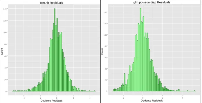
Figure 4. Deviance residuals for both models are approximately normally distributed. ... 14

Table 1. Listing of variable names and levels. ... 6

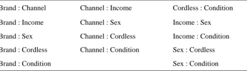
Table 2. 2-Way interactions included in both models. ... 7

Table 3. Test of over-dispersion results. ... 9

Table 4. Dissimilarity index values. Smaller values indicate better fit. ... 11

Table 5. Deviance and fit statistics for all fitted models. ... 11

Table 6. Inestimable parameters for both models. ... 15

Table 7. Interactions showing negative associations ... 18

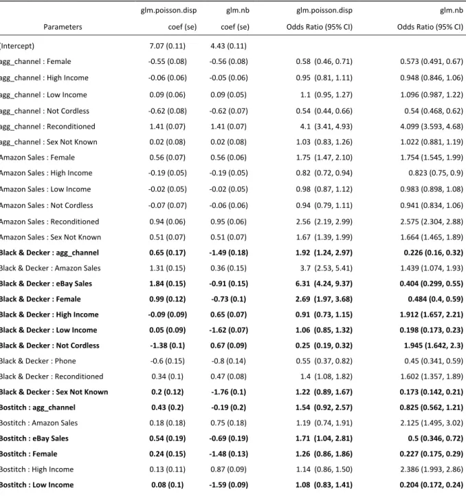
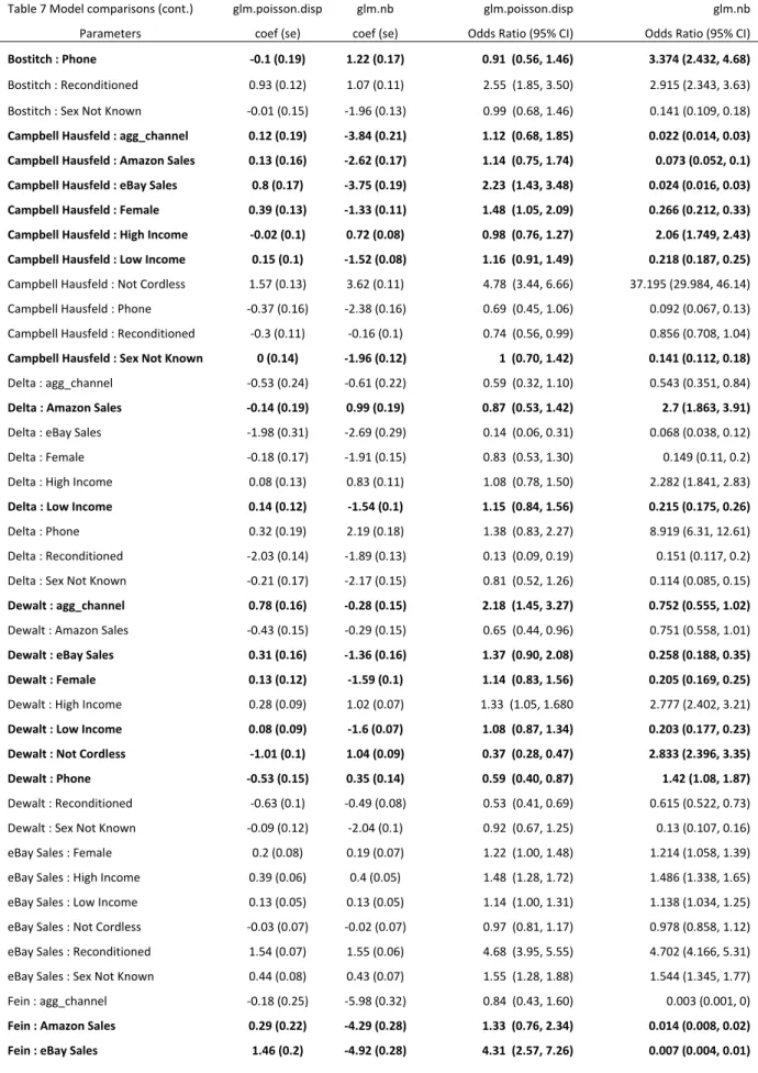
Table 8. Model comparisons. ... 21

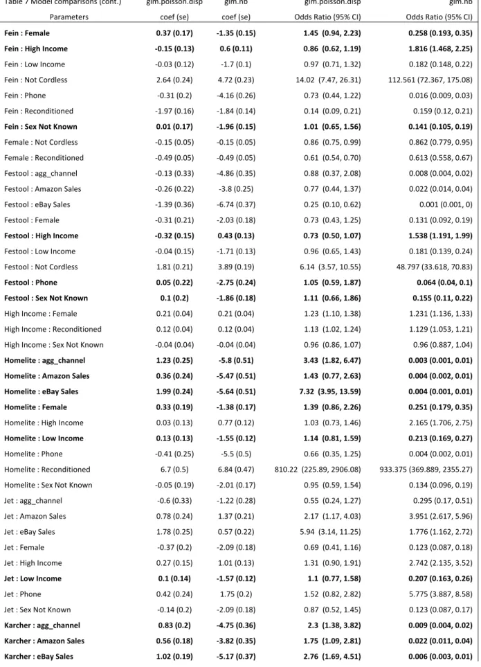
Table 9. Additional parameters output by glm.nb... 27

(5)

1. Introduction

For data that is well represented in a contingency table, by a table of counts, or where there is not a

distinct response variable, loglinear modeling is commonly employed to describe the direction and

magnitude of association between variables (Agresti 2007, Venables & Ripley 2002, McCullagh &

Nelder 1989

)

. It is especially useful for higher-order models or when the variables have many levels. All

of the above describe the data analyzed herein. See Jansakul and Hinde for a listing field application

and authors.

These data are sales data provided by an e-commerce company and include a wide variety of products

with mass appeal. As such, the sales frequencies for the many combinations of covariates can be vastly

different from one another. Such large differences make it difficult to account for the variance between

different covariate combinations. From the Comprehensive R Archive Network (CRAN,

http://CRAN.R-project.org/) comes two functions used to model such data:

glm.poisson.disp()

(in dispmod; Luca

Scrucca 2012, Breslow, N.E. 1984) and glm.nb() (in MASS; Venables, W. N. and Ripley, B. D. 2002).

While both model the data in valid ways—

glm.poisson.disp() using a Method of Moment (MM)

estimator of the parameters, and

glm.nb()

using Maximum Likelihood (ML)—and fit this data very

well, they often give opposing directions of association for covariate combinations. This paper briefly

discusses the effect on the model from using both R functions and the implications on inference if one is

chosen in lieu of another. In addition, results for the main research questions pertinent to the company

whose data are used are addressed in depth.

(6)

2. Background

In proposing the use of these data for this project, two areas of interest arose. The main question of

interest centered on what may influence how long an item stays in inventory of the company. Another aim

was to measure how, and in what way, the variables related to one another.

However, these data restricted direct analysis of this question because of the way “avg days in inv” is

calculated. It is an average of the days in inventory for all of the items of a specific type received by the

warehouse for any of the drops to the warehouse (a

drop

occurs twice a day and is when the system that

processes orders releases them to the warehouse for fulfillment). As such, this value may incorporate

storage time from different/multiple supplier shipments to the warehouse. Also, without distinction for

items that are drop shipped or pre-sale (put on sale before being received to the warehouse), there is no

clear way to distinguish in this analysis and beyond summary statistics if, or in what way, the average

days in inventory is affected by the characteristics of products or customers. Also, with respect to storage

time, because the data do not make distinctions among unique customers, there is no way to analyze

differences between specific combinations of customer characteristics related to particular products. Thus,

any interpretations of results from such an investigation may be spurious. However, what was able to be

addressed was the strength and direction of associations between a selected subset of variables.

(7)

3. Data

&

Methods

3.1 The Data

The original data file contained 1,186,929 observations. Each observation contains up to 25 variable

descriptions. From this file, SAS 9.2 was used for data management, reducing the number of variables to

six whose unique non-zero combinations were counted and exported using PROC SQL with analysis

carried out using R 2.11.1. There are 2,490 such combinations whose frequencies are studied.

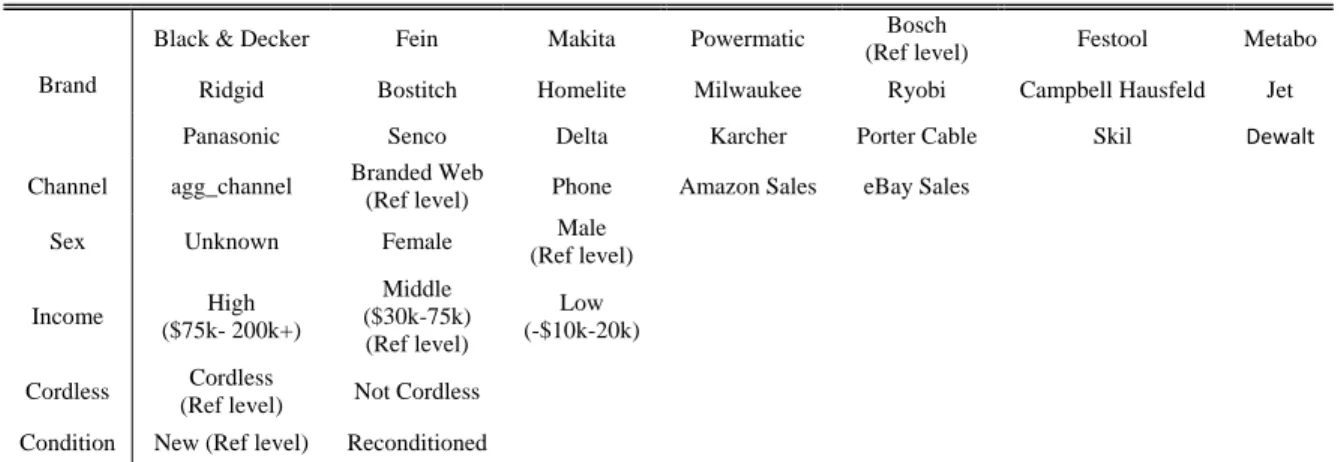
Below are the descriptions of the variable of interest. Each product manufacturer is listed under Brand.

Channel refers to the sales channel that the product is sold through. A

gg_channel

is comprised of Club

CPO: Phone, Club CPO: Web, Other, Outlets: Phone, Outlets: Web, Press.Wash: Phone, Press.Wash:

Web, Reconditioned Tools: Web, Reconditioned Tools: Phone, Tool Crib: Phone, Tool Crib: Web, and

Wholesale. A customer’s gender is given by Sex, and the original levels were aggregated as follows:

unknown

and

ambiguous

as Unknown;

female

and

probably female

as Female;

male

and

probably male

as

Male. A product’s sales condition is either New or Reconditioned. The descriptions for a tool being

cordless or corded are obvious.

Brand

Black & Decker Fein Makita Powermatic Bosch

(Ref level) Festool Metabo Ridgid Bostitch Homelite Milwaukee Ryobi Campbell Hausfeld Jet Panasonic Senco Delta Karcher Porter Cable Skil Dewalt

Channel agg_channel Branded Web _{(Ref level)} Phone Amazon Sales eBay Sales

Sex Unknown Female Male

(Ref level)

Income _{($75k- 200k+)}High

Middle ($30k-75k) (Ref level)

Low

(-$10k-20k)

Cordless Cordless

(Ref level) Not Cordless

Condition New (Ref level) Reconditioned

Table

1. Listing

of

variable

names

and

levels.

3.2 Methods

(8)

frequencies. It allows for interpretations of the strength and direction of relationships in these tables.

What is being modeled is the estimated

effect

on the frequency by unique groupings as shown by the

strength of the association between one or more variables in each group. As is the case in this analysis

where we have multiple two-variable interactions, the association between any two variables, given some

fixed level of the other four variables, has either a positive or negative effect on the expected number of

times this unique grouping appears in the data set. It may also be said that the effect on the estimated cell

frequency of one customer-product specification is

x

-times higher or lower when compared to the

reference group. Often, due to the complexity of interpretations or relevance, only one variable level at a

time will be adjusted. For instance, to compare different brands the remaining five variable levels will

remain the same for both brands; given these fixed levels, Brand A is associated with an increase

(decrease) in the estimated odds of a sale compared to Brand B.

The Poisson distribution assumes the mean and variance of the response are equal. The extra-variation,

referred to as extra-dispersion (in this case, strictly over-dispersion), inherent in this data violate this

assumption. This necessitates the need to estimate a dispersion parameter. Two methods for estimating

dispersion were used—glm.nb

and

glm.poisson.disp—because it was not clear to me how well

either would model the data.

Model selection was based forward/backward stepwise selection and ANOVA process to what difference

between the two functions there were and the interactions it deemed important. Stepwise selection for

both functions identified the Income by Cordless interaction for removal. ANOVA selection in glm.nb

further

identified the Sex x Cordless for removal. For comparative purposes the stepwise selections were

used.

The models estimated excluded the interaction between a person’s income and whether or not an item was

cordless. This exclusion implies conditional independence between these two variables given the other

variables, meaning that the association between the two variables does not depend on any others (Agresti

2007). The interactions included in both models are:

Brand

:

Channel

:

Income

Cordless

:

Condition

Brand

:

Income

Channel

:

Sex

Income

:

Sex

Brand

:

Sex

Channel

:

Cordless

Income

:

Condition

Brand

:

Cordless

Channel

:

Condition

Sex

:

Cordless

Brand

:

Condition

Sex

:

Condition

(9)

Since there are a prohibitive number of model parameters to express in an example of the model equation,

the general form for loglinear models is given next:

,

⋯

where

is the mean response of the effect

for covariates A and B, and where is the estimated

frequency of the mean response

, where is the and are the usual linear predictors.

3.3 Functions

glm.nb

This function uses an iteratively weighted least squares algorithm for estimating over-dispersion. A

benefit of glm.nb is that it defines the variance as a gamma random variable which, in allowing the

variance to be quadratic, better accounts for the tremendous variation in the observed data. Taking the

Poisson mean as a gamma distributed random variable leads to the NB model and we can obtain a

quadratic mean-variance relationship when the shape parameter is held constant and letting the scale

parameter vary (Jansakul and Hinde 2002)

.

Thus the negative binomial distribution is known as a

Poisson-Gamma mixture (Ma 2011).

For instance, suppose that the random variable represents frequencies of sales with means for each

combination of covariates in a fixed period of time. Because of the uncertainty in , it should itself be

regarded as a random variable. The following uses a parameterization given by Hinde and Dem

́trio

2007: The Poisson-Gamma mixture with

~

where

~

,

has a negative binomial

distribution for the :

| ,

Γ

!

,

0, 1, …

and

/

with

/ .

The estimation of

k

addresses over-dispersion, and is commonly denoted

. Note that by

(10)

glm.poisson.disp

The author of this function utilized an iterative algorithm that uses a moment method giving the unbiased

estimating equation (Breslow 1984)

1

0. This equates to solving Χ

where Χ

is the generalized Pearson Χ

statistic. Combining this with

weighted Poisson regression, Breslow proposed estimating using the weights,

1/ 1

̂ /

,

obtained from the previous iteration (Hinde and Dem

́trio).

3.4 Over-dispersion

Two potential causes of over-dispersion in this data may be that a variable for time and/or a variable for

customer location are not considered. Heterogeneity or dependence among clusters of data, whether

temporal or spatial, violates the Poisson assumption and can cause over-dispersion

(

Agresti 2007

)

. Figure

1 shows how spread out the data are. The range of sales frequencies is quite broad; there are 154 unique

covariate combinations appearing once, and a single unique observation appearing 48,245 times.

The mean of the frequency is 352.5261 with a variance of 2,473,575. While the data clearly violates

E

, Table 3 shows vastly different test statistics and similar, though not comparable, estimates

of the dispersion parameter . They are not directly comparable because both models estimated different

parameters due to singularities. These model differences are discussed in Section

4.4 and referenced, in

part, in the IBM

documentation.

Model Function Test

Stat

p-value

(se)

2-Way Interaction

glm.poisson.disp

_z

_{= 33.4573}

_{< 2.2e-16}

_{0.18798 (-)}

2-Way Interaction

glm.nb

½Χ

= 38365.1544

_{< 2.2e-16}

_{0.16107 (0.227)}

(11)

Figure

1. Distribution

of

counts

of

covariate

frequencies.

4. Model

Fit

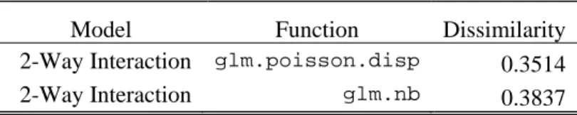
4.1 Dissimilarity

When checking the fit between models significant differences may be of little use because the large

sample size makes goodness-of-fit tests very sensitive in detecting the smallest effects. The Dissimilarity

Index (DI) summarizes the closeness of model fit irrespective of sample size. Its summary represents the

proportion of observations that need to be moved to create a perfect fit.

For a table of arbitrary dimension with cell counts

and fitted values

̂

, let

∑|

̂ |/2

∑|

|/2 , where takes values between 0 and 1. Smaller values of indicate

a better fitting model in a more practical sense (Agresti 2007). While this index is well suited for

comparing higher and lower order models, in this case it is used to help distinguish differences between

Distribution for Counts of Sales Frequency

Frequency

C

o

unt

0 50 100 150

(12)

the two functions. For these data, higher order models were either not relevant or significant enough to

consider. Table 4 shows that with a lower DI value the MM estimated model is slightly better than the

ML model. Also see Kuha and Firth 2010 for more information on the index.

Model Function

Dissimilarity

2-Way Interaction

glm.poisson.disp

_0.3514

2-Way Interaction

glm.nb

_0.3837

Table

4. Dissimilarity

index

values.

Smaller

values

indicate

better

fit.

4.2 Visual Model Fit

The moment estimated model has a lower deviance yielding a better, but somewhat heuristic, lack-of-fit

statistic (Table 5).

Model Function

AIC

Deviance

DF

LOF

(Dev/df)

All 2-Way Interactions

glm(...,family=Poisson)

60971

46682 2230 20.9336

Additive

glm.poisson.disp

2520

2026 2459 0.8239

2_Way (Reduced)

glm.poisson.disp

₄₆₀₂

₂₁₃₂

₂₂₃₂

_0.9552

Additive

glm.nb

25924

2751 2459 1.1187

2_Way (Reduced)

glm.nb

₂₂₆₂₂

₂₆₅₃

₂₂₃₂

_1.1882

Table

5. Deviance

and

fit

statistics

for

all

fitted

models.

(13)

Figure

2. ECDF

of

all

models.

Model Fit

Index

Em

p

ir

ic

a

l C

D

F

0.90

0.92

0.94

0.96

0.98

1.00 1000

2000

3000

4000

5000

Model Curve

Observed Frequency

glm.nb

glm.poisson.disp

glm.nb Interaction

(14)

Observed and Expected Sales Frequencies

Index

Sa

le

s

V

o

lu

m

e

0 2000

4000

6000

8000

10000

2300

2350

2400

2450

Model Curve

Observed Frequency

glm.nb Interaction

(15)

glm.nb Residuals Deviance Residuals C oun t 0 20 40 60 80 100 120 140

-4 -2 0 2 4

glm.poisson.disp Residuals Deviance Residuals Co u n t 0 20 40 60 80 100 120 140

-2 0 2 4

4.3 Model Assumptions

The boxplots of deviance residuals for the covariates show that, for each, no obvious trend is apparent

which indicates that the log transform of the baseline count was appropriate (Appendix 1-B.2,3 &

1-C.2,3) (Breslow 1995). Residual vs. Fitted plots given for both functions do not show evidence of

non-linearity, or unequal error variances. However, they both show three (different for each function) outliers,

but further investigation showed them to have no undue influence on parameter estimates (Appendix

1-B.1 and 1-C.1). Residual vs. Leverage plots did not show any substantial high-leverage points warranting

any action, though again, both functions identified different observations as being high-leverage

(Appendix 1-B.1 and 1-C.1). Further, DF Beta plots show no issues with highly influential observations

(Appendix 1-B.4 and 1-C.4). Also, there is no evidence of over-dispersion, or poor fit seen in the

Scale-Location plot for either function and the normal Q-Q plots (Appendix 1-B.1 and 1-C.1) show differing

results—that the ML model fits much better than the MM model—but Figure 4 shows that the deviance

residuals are approximately normal, again indicating correct model specification and model fit

(McCullagh & Nelder 1989, Lawless 1989).

(16)

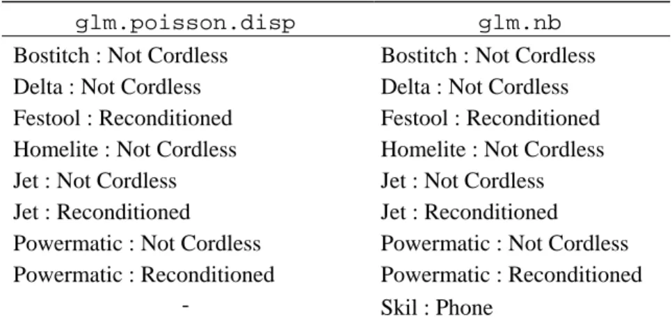
4.4 Differing Model Results

Both models contained parameters that were inestimable because of singularities in the Hessian matrix.

The

glm.nb

failed to estimate nine parameters while

glm.poisson.disp

did not estimate eight (Table

6).

glm.poisson.disp glm.nb

Bostitch : Not Cordless

Delta : Not Cordless

Festool : Reconditioned

Homelite : Not Cordless

Jet : Not Cordless

Jet : Reconditioned

Powermatic : Not Cordless

Powermatic : Reconditioned

-

Skil : Phone

Table

6. Inestimable

parameters

for

both

models.

One reason this may happen is because a variable(s) has only two levels. In most instances this is the

case, however, the singularities are not arising from the same parameters in both models. Since the

models are not estimating the same parameters, the effects of the covariates can be quite different

between models, i.e., one model may show a strong positive association, while the other, a strong

negative. To work around singularities stemming from this it may be possible to collapse levels, or

combine variables at the cost of losing information for other covariate combinations that are available. In

addition, the singularity may also arise from a mis-specified model. One aspect of the data that this

analysis does not address is the effect of time on the covariates, so it may be that the inclusion of this term

may aid in allowing for more estimable parameters.

The direction of many parameters differed between the two functions as well. For instance, of the 226

parameters estimated by both functions,

glm.poisson.disp

estimated 92 negative and 134 positive

associations, while

glm.nb

estimated 149 negative and 77 positive associations. Also, 42% of parameter

(17)

5. Results

As shown previously by Figure 4, the univariate standardized deviance residuals for both models have

comparable results that are listed next. Five brands that have the most variability are Ridgid, Dewalt,

Bostitch, Skil, and Porter Cable. Similarly brands with the least variability are Jet, Homelite, Makita, and

Milwaukee. The variability among

Sex

and

Income

is fairly similar across their respective levels, with

males and middle income persons showing slightly more variability in observed frequencies. Variability

among sales channels is greatest with

agg_channel

, least with

Branded Web,

and about the same across

Phone, Amazon,

and

eBay

.

Cordless

and

New

items exhibited greater variability than

Corded

and

Reconditioned

items, respectively.

Given the large number of comparisons that can be made between all of the variable levels, what is to

follow first is an outline of how any comparison between two variables using a conditional odds ratio may

be made along with the interpretation of the result. Second, this outline is also done for the odds ratio of

any single interaction with respect to the reference level. Third, in the case where one or more of the

variables in the interaction has only two levels, the odds ratios is a comparison of that group against the

reference group. Also note that the above comparisons should only be done if 1 is not in the 95%

confidence interval(s) (95%CI), as these do not indicate any significant difference between variable

levels.

Comparison between two variables using a conditional odds ratio



Divide the odds ratios of any two interactions that have (i) the exact same level of one variable,

and (ii) share the type of the other variable.

For instance, using estimates given by

glm.nb

, the association between Black & Decker items being sold

on eBay compared to Amazon holding all other variables fixed at the reference level (

male,

middle-income, and new, cordless

items) is given by

Black & ∶ Amazon Sales Odds Ratio

Black & :

1.439 . 404

3.562. This means that any

new

and c

ordless

Black & Decker item purchased by a

middle-income male

is about

3.6 times more likely to be sold on Amazon than it is on eBay. Similarly, the odds of a

new

and c

ordless

Black & Decker item purchased by a

middle-income male

on Amazon are about 256% higher than the

(18)

direction and magnitude of association—it is now a decrease for Amazon of about 41% compared to

eBay.

Interpreting an odds ratio with respect to the reference group



If the odds ratio of any interaction is below 1, then, with respect to the sales frequency, there is

evidence of a negative association between these variable levels when compared to the reference

group. If the odds ratio is greater than 1, then there is a positive association.



Any association for such cases represents the odds of being in the defined group rather than being

in the reference group.

This example uses the estimate from glm.nb. For instance, given the reference levels of a middle-income

male buying a new cordless item, the odds ratio for the interaction between Black & Decker and Phone,

0.55, represents a negative association between these variables and sales volume (frequency) when

compared to the sales volume expected from a middle-income male buying a new cordless item from

Bosch via the Branded Web site (Bosch and Branded Web are the reference levels for the variables).

More simply, this odds ratio is the odds of being in one group rather than another.

This ratio may also be interpreted in the following way: For any middle-income male buying a new

cordless Black & Decker item over the phone, there is a decrease in the predicted sales volume by a factor

of 0.55, or simply, a 45% decrease when compared to a Bosch item sold via the Branded Web site (for the

same any middle-income male buying a new cordless item).

The case were a variable(s) has only two levels

This is a more naturally understood case because the odds ratio represents the odds of being in group

rather than the other. This example uses the estimate from

glm.nb

. Consider the interaction between

(19)

The variables of interest are contained in the interactions listed in Table 2 and are restated here:

Brand : Channel Channel : Income Cordless : Condition Brand : Income Channel : Sex Income : Sex Brand : Sex Channel : Cordless Income : Condition Brand : Cordless Channel : Condition Sex : Cordless Brand : Condition Sex : Condition

Note again that the interaction between a person’s income level and an item being either cordless or not is

insignificant. That is, any combination of these two variables does not have an effect on sales volume.

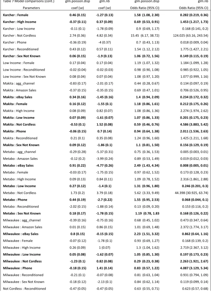
Assuming

glm.poisson.disp is used, Table 7 summarizes interactions having lower than expected

sales volumes (interactions where the variables are negatively associated). The interaction between

Brand

and

Channel

is not described because the frequency with which each combination appears is visually and

contextually convoluted.

Sex (female and/or unknown) :

Brand Bostitch Campbell Hausfeld Delta Dewalt Festool Homelite Jet Metabo Milwaukee Panasonic Powermatic Porter Cable Ridgid Skil

Channel agg_channel Phone Condition Reconditioned

Cordless Not Cordless Income High

Not Cordless :

Brand Black & Decker Dewalt Makita Milwaukee Panasonic Porter Cable Ridgid

Channel agg_channel eBay Condition Reconditioned

Sex Female Unknown

Reconditioned:

Brand Campbell Hausfeld Delta Dewalt Fein Metabo Milwaukee Panasonic Channel Phone

Cordless Not Cordless Income Low

Sex Unknown

Income (low and/or high) :

Brand Black & Decker Campbell Hausfeld Homelite Karcher Fein Festool Milwaukee Panasonic Ridgid Ryobi

Channel agg_channel Amazon

Condition Reconditioned

(20)

6. Discussion

Though the negative binomial model is more efficient and fully-defined compared to the moment method,

allowing for likelihood ratio tests, moment methods are more robust to issues of extra-dispersion

(Lawless 1987). Which is

better

may lie in one of the main areas yet to be assessed—an investigation into

independence between clusters of data and their correlations. Because temporal and spatial considerations

are not addressed through the inclusion of variables like time-of-sale, unique customer identification, or

geographical location, it is not clear that all variation is accounted for, or what effect their inclusion may

have on the results. Also, if singularities still occur after the inclusion of such covariates, then running

models repeatedly with and without each variable may be necessary to determine where they are coming

from. However, if these covariates are included, then, for example, prospective analyses, or profile

analysis may be utilized.

In addition, further investigation may show that when glm.poisson.disp and glm.nb estimate the

same model their results are indistinguishable from one another. It should also be noted that a

quasi-Poisson

model was estimated, and when the ECFs where compared, it appeared to fit better. Venables and

Ripley (2002) suggest the use of

quasi-

models. The only justification for choosing glm.poisson.disp

over

glm.nb is that it estimated one additional parameter. However, since glm.poisson.disp and

glm.nb

are quite different with respect to parameter estimates, it is recommended that a third function

using a

quasi-

likelihood method be tested so that some sort of validation of either the MM or ML model

can be made. As mentioned before, the visual fit of the

quasi-

method fit better, so it will likely be the

case that this method will be best, given the variables used.

7. Conclusion

Both

glm.nb

and

glm.poisson.disp

identified similar variables to estimate using stepwise selection

methods, but showed differences in the inestimable parameters in each model. Estimates of dispersion

parameters, and dissimilarity index (DI) values were relatively close to one another;

0.161 and

0.188 (Table 3), and shown by the DI values of 0.38 and 0.35 (Table 4), respectively. As

evidenced by the ECDF plot (Figure 2), model fit for the two functions is nearly identical. The notable

difference stems from the effect the unstable parameters due to singularities has on the measures of

associations:

glm.poisson.disp estimated 92 negative and 134 positive associations, while glm.nb

estimated 149 negative and 77 positive associations. That is, 42% of parameter estimates are going in

(21)

References

Agresti, Alan (2007).

Introduction to Categorical Data Analysis

. Second Edition. Wiley & Sons, New Jersey.

Aragan, J., D. Eberly and S. Eberly (1992).

Existence and Uniqueness of the Maximum Likelihood Estimator for the

Two-parameter Negative Binomial Distribution

. Statist. Probabil. Lett.,

15,

375-379.

Breslow, N.E.(1984).

Extra-Poisson Variation in Log-linear Models

. Appl. Statist.

33 No.1, 38-44.

Breslow, N.E.(1995).

Generalized Linear Models: Checking Assumptions and Strengthening Conclusions

. Prepared

for the Congresso Nazionale Societa’ Italiana di Biometrica. 16-17 June, 1995.

Lawless, J.F. (1987) Negative binomial and mixed Poisson regression.

Canadian Journal of Statistics

15 , 209-225.

McCullagh, P.,and Nelder,J .A. (1989).

Generalized Linear Models

. Second Edition. Chapman and Hall, London.

Venables, W.N. and Ripley, B.D. (2002)

Modern Applied Statistics with S

. Fourth Edition. Springer-Verlag, New

York.

Web References

Hinde, John and Dem

́

trio, Clarice G.B. Overdispersion: Models and Estimation. Lecture. Web 12 April, 2007.

Accessed 5 June, 2012.

<http://www.lce.esalq.usp.br/arquivos/aulas/2011/LCE5868/OverdispersionBook.pdf

>.

IBM. Unexpected singularities in the Hessian matrix in NOMREG (Multinomial Logistic Regression). Reference #:

1480408. Modified date: 2011-03-22. Web. 1 Aug. 2012.

<http://www-01.ibm.com/support/docview.wss?uid=swg21480408>.

Ismail , Norizura and Jemain, Abdyl Aziz. Handling Overdispersion with Negative Binomial and Generalized

Poisson Regression. Submitted Paper. Web 31 Jan. 2007.

<http://www.casact.org/pubs/forum/07wforum/07w109.pdf>.

Jansakul, Naratip and Hinde, John P. Linear Mean-Variance Negative Binomial Models

Applied to a Set of Orange Tissue-Culture Data. Submitted Paper. Web 2002. Accessed. 7 July, 2012.

<http://iceb.nccu.edu.tw/proceedings/APDSI/2002/papers/paper223.pdf>.

Kuha, Jouni and Firth, David (2010). On the Index of Dissimilarity for Lack Of Fit in Loglinear and

Log-multiplicative Models.

Computational Statistics and Data Analysis

55,

375-388. Web. 1 Sept. 2011.

Accessed 6 May, 2012.

<http://ac.els-cdn.com/S0167947310001921/1-s2.0-S0167947310001921-

main.pdf?_tid=5dfa0ca2-fdf9-11e1-b376-00000aacb35d&acdnat=1347578506_63e1f64a2ca8230133275f27be9f4817>.

Ma, Dan. The Negative Binomial Distribution.

A Blog on Probability and Statistics

. 11 July, 2011. Accessed 13

(22)

Appendix

1 ‐

A

Model

Comparisons:

Odds

Ratios

(95%

CI)

Table

8. Model comparisons.

1) glm.poisson.disp: 92 covariates have negative association; 134 have positive association. glm.nb: 149 covariates have negative association; 77 have positive association. Associations estimated in different directions are in bold.

2) 95% confidence intervals that include 1 are not significant at the 0.05 level.

3) Between glm.nb and glm.poisson.disp, 42% (95 of 226) of parameter estimates given by both models are in opposing directions. For glm.poisson.disp there were 92 covariates showing negative associations and 134 showing positive associations. For glm.nb

there were 149 covariates showing negative associations and 77 showing positive associations. 4) Estimates are rounded to the 2nd and 3rd decimal where appropriate to show that a 0 is not returned.

5) Parameters estimated by both models.

glm.poisson.disp glm.nb glm.poisson.disp glm.nb

Parameters coef (se) coef (se) Odds Ratio (95% CI) Odds Ratio (95% CI)

(Intercept) 7.07 (0.11) 4.43 (0.11)

agg_channel : Female ‐0.55 (0.08) ‐0.56 (0.08) 0.58 (0.46, 0.71) 0.573 (0.491, 0.67)

agg_channel : High Income ‐0.06 (0.06) ‐0.05 (0.06) 0.95 (0.81, 1.11) 0.948 (0.846, 1.06)

agg_channel : Low Income 0.09 (0.06) 0.09 (0.05) 1.1 (0.95, 1.27) 1.096 (0.987, 1.22)

agg_channel : Not Cordless ‐0.62 (0.08) ‐0.62 (0.07) 0.54 (0.44, 0.66) 0.54 (0.468, 0.62)

agg_channel : Reconditioned 1.41 (0.07) 1.41 (0.07) 4.1 (3.41, 4.93) 4.099 (3.593, 4.68)

agg_channel : Sex Not Known 0.02 (0.08) 0.02 (0.08) 1.03 (0.83, 1.26) 1.022 (0.881, 1.19)

Amazon Sales : Female 0.56 (0.07) 0.56 (0.06) 1.75 (1.47, 2.10) 1.754 (1.545, 1.99)

Amazon Sales : High Income ‐0.19 (0.05) ‐0.19 (0.05) 0.82 (0.72, 0.94) 0.823 (0.75, 0.9)

Amazon Sales : Low Income ‐0.02 (0.05) ‐0.02 (0.05) 0.98 (0.87, 1.12) 0.983 (0.898, 1.08)

Amazon Sales : Not Cordless ‐0.07 (0.07) ‐0.06 (0.06) 0.94 (0.79, 1.11) 0.941 (0.834, 1.06)

Amazon Sales : Reconditioned 0.94 (0.06) 0.95 (0.06) 2.56 (2.19, 2.99) 2.575 (2.304, 2.88)

Amazon Sales : Sex Not Known 0.51 (0.07) 0.51 (0.07) 1.67 (1.39, 1.99) 1.664 (1.465, 1.89)

Black & Decker : agg_channel 0.65 (0.17) ‐1.49 (0.18) 1.92 (1.24, 2.97) 0.226 (0.16, 0.32)

Black & Decker : Amazon Sales 1.31 (0.15) 0.36 (0.15) 3.7 (2.53, 5.41) 1.439 (1.074, 1.93)

Black & Decker : eBay Sales 1.84 (0.15) ‐0.91 (0.15) 6.31 (4.24, 9.37) 0.404 (0.299, 0.55)

Black & Decker : Female 0.99 (0.12) ‐0.73 (0.1) 2.69 (1.97, 3.68) 0.484 (0.4, 0.59)

Black & Decker : High Income ‐0.09 (0.09) 0.65 (0.07) 0.91 (0.73, 1.15) 1.912 (1.657, 2.21)

Black & Decker : Low Income 0.05 (0.09) ‐1.62 (0.07) 1.06 (0.85, 1.32) 0.198 (0.173, 0.23)

Black & Decker : Not Cordless ‐1.38 (0.1) 0.67 (0.09) 0.25 (0.19, 0.32) 1.945 (1.642, 2.3)

Black & Decker : Phone ‐0.6 (0.15) ‐0.8 (0.14) 0.55 (0.37, 0.82) 0.45 (0.341, 0.59)

Black & Decker : Reconditioned 0.34 (0.1) 0.47 (0.08) 1.4 (1.08, 1.82) 1.602 (1.357, 1.89)

Black & Decker : Sex Not Known 0.2 (0.12) ‐1.76 (0.1) 1.22 (0.89, 1.67) 0.173 (0.142, 0.21)

Bostitch : agg_channel 0.43 (0.2) ‐0.19 (0.2) 1.54 (0.92, 2.57) 0.825 (0.562, 1.21)

Bostitch : Amazon Sales 0.18 (0.18) 0.75 (0.18) 1.19 (0.74, 1.91) 2.125 (1.495, 3.02)

Bostitch : eBay Sales 0.54 (0.19) ‐0.69 (0.19) 1.71 (1.04, 2.81) 0.5 (0.346, 0.72)

Bostitch : Female 0.24 (0.15) ‐1.48 (0.13) 1.26 (0.86, 1.86) 0.227 (0.175, 0.29)

(23)

Table 7 Model comparisons (cont.) glm.poisson.disp glm.nb glm.poisson.disp glm.nb

Bostitch : Phone ‐0.1 (0.19) 1.22 (0.17) 0.91 (0.56, 1.46) 3.374 (2.432, 4.68)

Bostitch : Reconditioned 0.93 (0.12) 1.07 (0.11) 2.55 (1.85, 3.50) 2.915 (2.343, 3.63)

Bostitch : Sex Not Known ‐0.01 (0.15) ‐1.96 (0.13) 0.99 (0.68, 1.46) 0.141 (0.109, 0.18)

Campbell Hausfeld : agg_channel 0.12 (0.19) ‐3.84 (0.21) 1.12 (0.68, 1.85) 0.022 (0.014, 0.03)

Campbell Hausfeld : Amazon Sales 0.13 (0.16) ‐2.62 (0.17) 1.14 (0.75, 1.74) 0.073 (0.052, 0.1)

Campbell Hausfeld : eBay Sales 0.8 (0.17) ‐3.75 (0.19) 2.23 (1.43, 3.48) 0.024 (0.016, 0.03)

Campbell Hausfeld : Female 0.39 (0.13) ‐1.33 (0.11) 1.48 (1.05, 2.09) 0.266 (0.212, 0.33)

Campbell Hausfeld : High Income ‐0.02 (0.1) 0.72 (0.08) 0.98 (0.76, 1.27) 2.06 (1.749, 2.43)

Campbell Hausfeld : Low Income 0.15 (0.1) ‐1.52 (0.08) 1.16 (0.91, 1.49) 0.218 (0.187, 0.25)

Campbell Hausfeld : Not Cordless 1.57 (0.13) 3.62 (0.11) 4.78 (3.44, 6.66) 37.195 (29.984, 46.14)

Campbell Hausfeld : Phone ‐0.37 (0.16) ‐2.38 (0.16) 0.69 (0.45, 1.06) 0.092 (0.067, 0.13)

Campbell Hausfeld : Reconditioned ‐0.3 (0.11) ‐0.16 (0.1) 0.74 (0.56, 0.99) 0.856 (0.708, 1.04)

Campbell Hausfeld : Sex Not Known 0 (0.14) ‐1.96 (0.12) 1 (0.70, 1.42) 0.141 (0.112, 0.18)

Delta : agg_channel ‐0.53 (0.24) ‐0.61 (0.22) 0.59 (0.32, 1.10) 0.543 (0.351, 0.84)

Delta : Amazon Sales ‐0.14 (0.19) 0.99 (0.19) 0.87 (0.53, 1.42) 2.7 (1.863, 3.91)

Delta : eBay Sales ‐1.98 (0.31) ‐2.69 (0.29) 0.14 (0.06, 0.31) 0.068 (0.038, 0.12)

Delta : Female ‐0.18 (0.17) ‐1.91 (0.15) 0.83 (0.53, 1.30) 0.149 (0.11, 0.2)

Delta : High Income 0.08 (0.13) 0.83 (0.11) 1.08 (0.78, 1.50) 2.282 (1.841, 2.83)

Delta : Low Income 0.14 (0.12) ‐1.54 (0.1) 1.15 (0.84, 1.56) 0.215 (0.175, 0.26)

Delta : Phone 0.32 (0.19) 2.19 (0.18) 1.38 (0.83, 2.27) 8.919 (6.31, 12.61)

Delta : Reconditioned ‐2.03 (0.14) ‐1.89 (0.13) 0.13 (0.09, 0.19) 0.151 (0.117, 0.2)

Delta : Sex Not Known ‐0.21 (0.17) ‐2.17 (0.15) 0.81 (0.52, 1.26) 0.114 (0.085, 0.15)

Dewalt : agg_channel 0.78 (0.16) ‐0.28 (0.15) 2.18 (1.45, 3.27) 0.752 (0.555, 1.02)

Dewalt : Amazon Sales ‐0.43 (0.15) ‐0.29 (0.15) 0.65 (0.44, 0.96) 0.751 (0.558, 1.01)

Dewalt : eBay Sales 0.31 (0.16) ‐1.36 (0.16) 1.37 (0.90, 2.08) 0.258 (0.188, 0.35)

Dewalt : Female 0.13 (0.12) ‐1.59 (0.1) 1.14 (0.83, 1.56) 0.205 (0.169, 0.25)

Dewalt : High Income 0.28 (0.09) 1.02 (0.07) 1.33 (1.05, 1.680 2.777 (2.402, 3.21)

Dewalt : Low Income 0.08 (0.09) ‐1.6 (0.07) 1.08 (0.87, 1.34) 0.203 (0.177, 0.23)

Dewalt : Not Cordless ‐1.01 (0.1) 1.04 (0.09) 0.37 (0.28, 0.47) 2.833 (2.396, 3.35)

Dewalt : Phone ‐0.53 (0.15) 0.35 (0.14) 0.59 (0.40, 0.87) 1.42 (1.08, 1.87)

Dewalt : Reconditioned ‐0.63 (0.1) ‐0.49 (0.08) 0.53 (0.41, 0.69) 0.615 (0.522, 0.73)

Dewalt : Sex Not Known ‐0.09 (0.12) ‐2.04 (0.1) 0.92 (0.67, 1.25) 0.13 (0.107, 0.16)

eBay Sales : Female 0.2 (0.08) 0.19 (0.07) 1.22 (1.00, 1.48) 1.214 (1.058, 1.39)

eBay Sales : High Income 0.39 (0.06) 0.4 (0.05) 1.48 (1.28, 1.72) 1.486 (1.338, 1.65)

eBay Sales : Low Income 0.13 (0.05) 0.13 (0.05) 1.14 (1.00, 1.31) 1.138 (1.034, 1.25)

eBay Sales : Not Cordless ‐0.03 (0.07) ‐0.02 (0.07) 0.97 (0.81, 1.17) 0.978 (0.858, 1.12)

eBay Sales : Reconditioned 1.54 (0.07) 1.55 (0.06) 4.68 (3.95, 5.55) 4.702 (4.166, 5.31)

eBay Sales : Sex Not Known 0.44 (0.08) 0.43 (0.07) 1.55 (1.28, 1.88) 1.544 (1.345, 1.77)

Fein : agg_channel ‐0.18 (0.25) ‐5.98 (0.32) 0.84 (0.43, 1.60) 0.003 (0.001, 0)

Fein : Amazon Sales 0.29 (0.22) ‐4.29 (0.28) 1.33 (0.76, 2.34) 0.014 (0.008, 0.02)

(24)

Fein : Female 0.37 (0.17) ‐1.35 (0.15) 1.45 (0.94, 2.23) 0.258 (0.193, 0.35)

Fein : High Income ‐0.15 (0.13) 0.6 (0.11) 0.86 (0.62, 1.19) 1.816 (1.468, 2.25)

Fein : Low Income ‐0.03 (0.12) ‐1.7 (0.1) 0.97 (0.71, 1.32) 0.182 (0.148, 0.22)

Fein : Not Cordless 2.64 (0.24) 4.72 (0.23) 14.02 (7.47, 26.31) 112.561 (72.367, 175.08)

Fein : Phone ‐0.31 (0.2) ‐4.16 (0.26) 0.73 (0.44, 1.22) 0.016 (0.009, 0.03)

Fein : Reconditioned ‐1.97 (0.16) ‐1.84 (0.14) 0.14 (0.09, 0.21) 0.159 (0.12, 0.21)

Fein : Sex Not Known 0.01 (0.17) ‐1.96 (0.15) 1.01 (0.65, 1.56) 0.141 (0.105, 0.19)

Female : Not Cordless ‐0.15 (0.05) ‐0.15 (0.05) 0.86 (0.75, 0.99) 0.862 (0.779, 0.95)

Female : Reconditioned ‐0.49 (0.05) ‐0.49 (0.05) 0.61 (0.54, 0.70) 0.613 (0.558, 0.67)

Festool : agg_channel ‐0.13 (0.33) ‐4.86 (0.35) 0.88 (0.37, 2.08) 0.008 (0.004, 0.02)

Festool : Amazon Sales ‐0.26 (0.22) ‐3.8 (0.25) 0.77 (0.44, 1.37) 0.022 (0.014, 0.04)

Festool : eBay Sales ‐1.39 (0.36) ‐6.74 (0.37) 0.25 (0.10, 0.62) 0.001 (0.001, 0)

Festool : Female ‐0.31 (0.21) ‐2.03 (0.18) 0.73 (0.43, 1.25) 0.131 (0.092, 0.19)

Festool : High Income ‐0.32 (0.15) 0.43 (0.13) 0.73 (0.50, 1.07) 1.538 (1.191, 1.99)

Festool : Low Income ‐0.04 (0.15) ‐1.71 (0.13) 0.96 (0.65, 1.43) 0.181 (0.139, 0.24)

Festool : Not Cordless 1.81 (0.21) 3.89 (0.19) 6.14 (3.57, 10.55) 48.797 (33.618, 70.83)

Festool : Phone 0.05 (0.22) ‐2.75 (0.24) 1.05 (0.59, 1.87) 0.064 (0.04, 0.1)

Festool : Sex Not Known 0.1 (0.2) ‐1.86 (0.18) 1.11 (0.66, 1.86) 0.155 (0.11, 0.22)

High Income : Female 0.21 (0.04) 0.21 (0.04) 1.23 (1.10, 1.38) 1.231 (1.136, 1.33)

High Income : Reconditioned 0.12 (0.04) 0.12 (0.04) 1.13 (1.02, 1.24) 1.129 (1.053, 1.21)

High Income : Sex Not Known ‐0.04 (0.04) ‐0.04 (0.04) 0.96 (0.86, 1.07) 0.96 (0.887, 1.04)

Homelite : agg_channel 1.23 (0.25) ‐5.8 (0.51) 3.43 (1.82, 6.47) 0.003 (0.001, 0.01)

Homelite : Amazon Sales 0.36 (0.24) ‐5.47 (0.51) 1.43 (0.77, 2.63) 0.004 (0.002, 0.01)

Homelite : eBay Sales 1.99 (0.24) ‐5.64 (0.51) 7.32 (3.95, 13.59) 0.004 (0.001, 0.01)

Homelite : Female 0.33 (0.19) ‐1.38 (0.17) 1.39 (0.86, 2.26) 0.251 (0.179, 0.35)

Homelite : High Income 0.03 (0.13) 0.77 (0.12) 1.03 (0.73, 1.46) 2.165 (1.706, 2.75)

Homelite : Low Income 0.13 (0.13) ‐1.55 (0.12) 1.14 (0.81, 1.59) 0.213 (0.169, 0.27)

Homelite : Phone ‐0.41 (0.25) ‐5.5 (0.5) 0.66 (0.35, 1.25) 0.004 (0.002, 0.01)

Homelite : Reconditioned 6.7 (0.5) 6.84 (0.47) 810.22 (225.89, 2906.08) 933.375 (369.889, 2355.27)

Homelite : Sex Not Known ‐0.05 (0.19) ‐2.01 (0.17) 0.95 (0.59, 1.54) 0.134 (0.096, 0.19)

Jet : agg_channel ‐0.6 (0.33) ‐1.22 (0.28) 0.55 (0.24, 1.27) 0.295 (0.17, 0.51)

Jet : Amazon Sales 0.78 (0.24) 1.37 (0.21) 2.17 (1.17, 4.03) 3.951 (2.617, 5.96)

Jet : eBay Sales 1.78 (0.25) 0.57 (0.22) 5.94 (3.14, 11.25) 1.776 (1.162, 2.72)

Jet : Female ‐0.37 (0.2) ‐2.09 (0.18) 0.69 (0.41, 1.16) 0.123 (0.087, 0.18)

Jet : High Income 0.27 (0.15) 1.01 (0.13) 1.31 (0.90, 1.91) 2.742 (2.135, 3.52)

Jet : Low Income 0.1 (0.14) ‐1.57 (0.12) 1.1 (0.77, 1.58) 0.207 (0.163, 0.26)

Jet : Phone 0.42 (0.24) 1.75 (0.2) 1.52 (0.82, 2.82) 5.775 (3.887, 8.58)

Jet : Sex Not Known ‐0.14 (0.2) ‐2.09 (0.18) 0.87 (0.52, 1.45) 0.123 (0.087, 0.17)

Karcher : agg_channel 0.83 (0.2) ‐4.75 (0.36) 2.3 (1.38, 3.82) 0.009 (0.004, 0.02)

(25)

Karcher : Female 0.46 (0.15) ‐1.27 (0.13) 1.58 (1.08, 2.30) 0.282 (0.219, 0.36)

Karcher : High Income ‐0.37 (0.11) 0.37 (0.09) 0.69 (0.53, 0.91) 1.453 (1.217, 1.73)

Karcher : Low Income ‐0.11 (0.1) ‐1.78 (0.09) 0.9 (0.69, 1.17) 0.168 (0.141, 0.2)

Karcher : Not Cordless 2.74 (0.36) 4.82 (0.34) 15.45 (6.17, 38.72) 124.025 (63.16, 243.54)

Karcher : Phone ‐0.36 (0.19) ‐4 (0.37) 0.7 (0.43, 1.13) 0.018 (0.009, 0.04)

Karcher : Reconditioned 0.43 (0.12) 0.57 (0.11) 1.54 (1.12, 2.12) 1.775 (1.427, 2.21)

Karcher : Sex Not Known 0.06 (0.15) ‐1.9 (0.13) 1.06 (0.72, 1.56) 0.149 (0.115, 0.19)

Low Income : Female 0.17 (0.04) 0.17 (0.04) 1.19 (1.07, 1.32) 1.184 (1.099, 1.28)

Low Income : Reconditioned ‐0.02 (0.04) ‐0.02 (0.03) 0.98 (0.90, 1.08) 0.985 (0.922, 1.05)

Low Income : Sex Not Known 0.08 (0.04) 0.07 (0.04) 1.08 (0.97, 1.20) 1.077 (0.999, 1.16)

Makita : agg_channel ‐0.83 (0.17) ‐2.01 (0.17) 0.44 (0.28, 0.67) 0.134 (0.097, 0.19)

Makita : Amazon Sales ‐0.37 (0.15) ‐0.35 (0.15) 0.69 (0.47, 1.01) 0.706 (0.526, 0.95)

Makita : eBay Sales 0.34 (0.16) ‐1.45 (0.16) 1.4 (0.94, 2.09) 0.234 (0.172, 0.32)

Makita : Female 0.16 (0.12) ‐1.55 (0.1) 1.18 (0.86, 1.61) 0.212 (0.175, 0.26)

Makita : High Income 0.08 (0.09) 0.82 (0.07) 1.08 (0.86, 1.36) 2.274 (1.974, 2.62)

Makita : Low Income 0.07 (0.09) ‐1.61 (0.07) 1.07 (0.86, 1.33) 0.201 (0.175, 0.23)

Makita : Not Cordless ‐0.53 (0.1) 1.52 (0.08) 0.59 (0.46, 0.76) 4.586 (3.883, 5.42)

Makita : Phone ‐0.06 (0.15) 0.7 (0.14) 0.94 (0.64, 1.38) 2.011 (1.536, 2.63)

Makita : Reconditioned 0.21 (0.1) 0.35 (0.08) 1.24 (0.96, 1.60) 1.425 (1.211, 1.68)

Makita : Sex Not Known 0.09 (0.12) ‐1.86 (0.1) 1.1 (0.81, 1.50) 0.156 (0.129, 0.19)

Metabo : agg_channel ‐0.29 (0.28) ‐5.37 (0.31) 0.75 (0.36, 1.53) 0.005 (0.003, 0.01)

Metabo : Amazon Sales ‐0.12 (0.2) ‐3.99 (0.24) 0.89 (0.53, 1.49) 0.019 (0.012, 0.03)

Metabo : eBay Sales 0.91 (0.22) ‐4.77 (0.26) 2.49 (1.43, 4.34) 0.008 (0.005, 0.01)

Metabo : Female ‐0.03 (0.17) ‐1.75 (0.15) 0.97 (0.62, 1.52) 0.173 (0.128, 0.23)

Metabo : High Income 0.09 (0.13) 0.84 (0.11) 1.09 (0.78, 1.52) 2.316 (1.861, 2.88)

Metabo : Low Income 0.27 (0.12) ‐1.4 (0.1) 1.31 (0.96, 1.80) 0.246 (0.201, 0.3)

Metabo : Not Cordless 1.73 (0.2) 3.79 (0.18) 5.62 (3.33, 9.49) 44.398 (30.925, 63.74)

Metabo : Phone 0.44 (0.19) ‐2.7 (0.22) 1.55 (0.95, 2.53) 0.068 (0.044, 0.1)

Metabo : Reconditioned ‐2.02 (0.15) ‐1.88 (0.14) 0.13 (0.09, 0.20) 0.153 (0.116, 0.2)

Metabo : Sex Not Known 0.18 (0.17) ‐1.78 (0.15) 1.19 (0.78, 1.83 0.168 (0.126, 0.22)

Milwaukee : agg_channel ‐0.39 (0.16) ‐0.75 (0.16) 0.68 (0.45, 1.02) 0.473 (0.347, 0.64)

Milwaukee : Amazon Sales 0.01 (0.15) 0.86 (0.15) 1.01 (0.69, 1.48) 2.372 (1.774, 3.17)

Milwaukee : eBay Sales 0.8 (0.15) ‐0.15 (0.15) 2.23 (1.51, 3.32) 0.862 (0.64, 1.16)

Milwaukee : Female ‐0.07 (0.12) ‐1.78 (0.1) 0.93 (0.69, 1.27) 0.168 (0.139, 0.2)

Milwaukee : High Income 0.26 (0.09) 1 (0.07) 1.3 (1.04, 1.62) 2.719 (2.367, 3.12)

Milwaukee : Low Income 0.05 (0.08) ‐1.62 (0.07) 1.05 (0.85, 1.30) 0.197 (0.173, 0.23)

Milwaukee : Not Cordless ‐1.23 (0.1) 0.82 (0.08) 0.29 (0.23, 0.38) 2.263 (1.921, 2.67)

Milwaukee : Phone ‐0.18 (0.15) 1.41 (0.14) 0.83 (0.57, 1.22) 4.087 (3.129, 5.34)

Milwaukee : Reconditioned ‐0.21 (0.1) ‐0.07 (0.08) 0.81 (0.63, 1.04) 0.931 (0.794, 1.09)

Milwaukee : Sex Not Known ‐0.18 (0.12) ‐2.13 (0.1) 0.84 (0.62, 1.14) 0.119 (0.099, 0.14)

(26)

Panasonic : agg_channel 0.56 (0.26) ‐3.11 (0.25) 1.76 (0.89, 3.46) 0.045 (0.027, 0.07)

Panasonic : Amazon Sales 1.08 (0.18) ‐1.36 (0.18) 2.95 (1.86, 4.68) 0.256 (0.181, 0.36)

Panasonic : eBay Sales 1.25 (0.22) ‐3.01 (0.21) 3.48 (1.96, 6.21) 0.049 (0.032, 0.07)

Panasonic : Female ‐0.06 (0.17) ‐1.78 (0.15) 0.95 (0.60, 1.48) 0.169 (0.125, 0.23)

Panasonic : High Income ‐0.02 (0.13) 0.72 (0.12) 0.98 (0.69, 1.38) 2.059 (1.635, 2.59)

Panasonic : Low Income 0.14 (0.12) ‐1.54 (0.11) 1.15 (0.83, 1.58) 0.214 (0.173, 0.27)

Panasonic : Not Cordless ‐2.35 (0.14) ‐0.31 (0.12) 0.1 (0.07, 0.14) 0.734 (0.58, 0.93)

Panasonic : Phone 0.03 (0.2) ‐1.69 (0.18) 1.03 (0.61, 1.74) 0.185 (0.13, 0.26)

Panasonic : Reconditioned ‐1.31 (0.14) ‐1.17 (0.12) 0.27 (0.19, 0.39) 0.309 (0.244, 0.39)

Panasonic : Sex Not Known 0.27 (0.17) ‐1.7 (0.14) 1.31 (0.85, 2.01) 0.184 (0.138, 0.24)

Phone : Female ‐0.04 (0.07) ‐0.04 (0.07) 0.96 (0.80, 1.16) 0.962 (0.845, 1.1)

Phone : High Income 0.15 (0.05) 0.15 (0.05) 1.16 (1.01, 1.33) 1.157 (1.051, 1.28)

Phone : Low Income 0.11 (0.05) 0.11 (0.05) 1.11 (0.98, 1.27) 1.112 (1.014, 1.22)

Phone : Not Cordless 0 (0.07) 0.01 (0.06) 1 (0.84, 1.19) 1.007 (0.89, 1.14)

Phone : Reconditioned ‐0.18 (0.06) ‐0.18 (0.06) 0.83 (0.71, 0.98) 0.832 (0.743, 0.93)

Phone : Sex Not Known ‐0.05 (0.07) ‐0.06 (0.07) 0.95 (0.79, 1.14) 0.946 (0.829, 1.08)

Porter Cable : agg_channel 0.2 (0.16) ‐1.3 (0.17) 1.22 (0.80, 1.86) 0.271 (0.196, 0.38)

Porter Cable : Amazon Sales ‐0.65 (0.15) ‐0.96 (0.15) 0.52 (0.35, 0.77) 0.384 (0.284, 0.52)

Porter Cable : eBay Sales ‐0.37 (0.17) ‐2.49 (0.18) 0.69 (0.45, 1.08) 0.083 (0.059, 0.12)

Porter Cable : Female 0.13 (0.12) ‐1.59 (0.1) 1.13 (0.82, 1.56) 0.203 (0.167, 0.25)

Porter Cable : High Income 0.12 (0.09) 0.86 (0.07) 1.12 (0.89, 1.42) 2.352 (2.032, 2.72)

Porter Cable : Low Income 0.11 (0.09) ‐1.56 (0.07) 1.12 (0.89, 1.40) 0.21 (0.183, 0.24)

Porter Cable : Not Cordless ‐0.13 (0.1) 1.93 (0.09) 0.88 (0.67, 1.15) 6.865 (5.78, 8.15)

Porter Cable : Phone ‐0.08 (0.15) 0.35 (0.14) 0.92 (0.62, 1.35) 1.425 (1.084, 1.87)

Porter Cable : Reconditioned 0.01 (0.1) 0.15 (0.09) 1.01 (0.78, 1.32) 1.163 (0.982, 1.38)

Porter Cable : Sex Not Known ‐0.22 (0.12) ‐2.18 (0.1) 0.8 (0.58, 1.10) 0.113 (0.093, 0.14)

Powermatic : agg_channel 0.23 (0.42) ‐2.35 (0.36) 1.26 (0.43, 3.67) 0.096 (0.047, 0.19)

Powermatic : Amazon Sales 1.79 (0.26) 0.41 (0.22) 6.01 (3.08, 11.75) 1.512 (0.976, 2.34)

Powermatic : eBay Sales 1.1 (0.33) ‐2.1 (0.29) 2.99 (1.27, 7.04) 0.123 (0.07, 0.22)

Powermatic : Female ‐0.82 (0.24) ‐2.54 (0.22) 0.44 (0.24, 0.82) 0.079 (0.051, 0.12)

Powermatic : High Income 0.14 (0.18) 0.86 (0.16) 1.15 (0.73, 1.80) 2.375 (1.741, 3.24)

Powermatic : Low Income ‐0.16 (0.16) ‐1.83 (0.15) 0.85 (0.56, 1.30) 0.16 (0.12, 0.21)

Powermatic : Phone 1.19 (0.26) 0.55 (0.22) 3.28 (1.66, 6.48) 1.733 (1.134, 2.65)

Powermatic : Sex Not Known ‐0.44 (0.23) ‐2.39 (0.21) 0.65 (0.35, 1.18) 0.091 (0.06, 0.14)

Ridgid : agg_channel 0.93 (0.17) ‐1.76 (0.17) 2.53 (1.63, 3.93) 0.172 (0.123, 0.24)

Ridgid : Amazon Sales 0.23 (0.16) ‐1.25 (0.16) 1.26 (0.84, 1.900 0.288 (0.21, 0.39)

Ridgid : eBay Sales 1.53 (0.17) ‐1.75 (0.18) 4.63 (3.00, 7.15) 0.173 (0.122, 0.25)

Ridgid : Female ‐0.01 (0.13) ‐1.73 (0.11) 0.99 (0.71, 1.39) 0.178 (0.144, 0.22)

Ridgid : High Income 0.13 (0.1) 0.87 (0.08) 1.14 (0.88, 1.47) 2.388 (2.028, 2.81)

(27)

Ridgid : Phone ‐0.43 (0.17) ‐1.17 (0.16) 0.65 (0.42, 1.00) 0.31 (0.226, 0.42)

Ridgid : Reconditioned 0.63 (0.11) 0.77 (0.1) 1.88 (1.41, 2.51) 2.169 (1.796, 2.62)

Ridgid : Sex Not Known ‐0.16 (0.13) ‐2.11 (0.11) 0.86 (0.61, 1.20) 0.121 (0.098, 0.15)

Ryobi : agg_channel 0.52 (0.18) ‐3.89 (0.21) 1.68 (1.06, 2.65) 0.02 (0.014, 0.03)

Ryobi : Amazon Sales 0.67 (0.16) ‐2.55 (0.19) 1.95 (1.28, 2.95) 0.078 (0.054, 0.11)

Ryobi : eBay Sales 1.72 (0.17) ‐3.31 (0.19) 5.56 (3.62, 8.53) 0.037 (0.025, 0.05)

Ryobi : Female 0.37 (0.13) ‐1.35 (0.11) 1.44 (1.03, 2.02) 0.259 (0.208, 0.32)

Ryobi : High Income 0 (0.1) 0.74 (0.08) 1 (0.78, 1.27) 2.09 (1.779, 2.45)

Ryobi : Low Income 0.07 (0.09) ‐1.61 (0.08) 1.07 (0.84, 1.36) 0.201 (0.172, 0.23)

Ryobi : Not Cordless 1.05 (0.12) 3.1 (0.11) 2.84 (2.07, 3.91) 22.099 (17.685, 27.61)

Ryobi : Phone ‐0.78 (0.17) ‐3.25 (0.18) 0.46 (0.30, 0.71) 0.039 (0.027, 0.06)

Ryobi : Reconditioned 2.09 (0.12) 2.23 (0.11) 8.09 (5.87, 11.16) 9.267 (7.431, 11.56)

Ryobi : Sex Not Known 0.03 (0.13) ‐1.92 (0.11) 1.03 (0.73, 1.45) 0.146 (0.117, 0.18)

Senco : agg_channel 0.43 (0.21) ‐4.73 (0.23) 1.54 (0.90, 2.64) 0.009 (0.006, 0.01)

Senco : Amazon Sales 0.54 (0.17) ‐3.41 (0.19) 1.72 (1.11, 2.66) 0.033 (0.023, 0.05)

Senco : eBay Sales 1.15 (0.19) ‐4.61 (0.21) 3.16 (1.96, 5.09) 0.01 (0.007, 0.01)

Senco : Female 0.03 (0.15) ‐1.69 (0.13) 1.03 (0.71, 1.49) 0.184 (0.143, 0.24)

Senco : High Income 0.27 (0.11) 1.01 (0.1) 1.31 (0.98, 1.74) 2.744 (2.273, 3.31)

Senco : Low Income 0.09 (0.1) ‐1.59 (0.09) 1.09 (0.84, 1.42) 0.205 (0.173, 0.24)

Senco : Not Cordless 0.87 (0.13) 2.93 (0.12) 2.4 (1.70, 3.39) 18.692 (14.782, 23.64)

Senco : Phone 0.16 (0.18) ‐3.05 (0.18) 1.17 (0.75, 1.85) 0.047 (0.033, 0.07)

Senco : Reconditioned 0.76 (0.12) 0.89 (0.11) 2.13 (1.55, 2.93) 2.445 (1.975, 3.03)

Senco : Sex Not Known ‐0.16 (0.15) ‐2.11 (0.13) 0.85 (0.58, 1.24) 0.121 (0.094, 0.16)

Sex Not Known : Not Cordless ‐0.1 (0.06) ‐0.1 (0.05) 0.9 (0.78, 1.04) 0.907 (0.819, 1)

Sex Not Known : Reconditioned ‐0.11 (0.05) ‐0.1 (0.05) 0.9 (0.79, 1.02) 0.901 (0.82, 0.99)

Skil : agg_channel ‐0.27 (0.16) ‐1.81 (0.14) 0.76 (0.50, 1.16) 0.163 (0.125, 0.21)

Skil : Amazon Sales ‐0.11 (0.15) ‐0.45 (0.12) 0.89 (0.61, 1.31) 0.637 (0.505, 0.8)

Skil : eBay Sales 0.59 (0.15) ‐1.56 (0.12) 1.8 (1.21, 2.68) 0.21 (0.164, 0.27)

Skil : Female 0.57 (0.12) ‐1.15 (0.1) 1.77 (1.30, 2.41) 0.317 (0.263, 0.38)

Skil : High Income 0.14 (0.09) 0.88 (0.07) 1.15 (0.92, 1.45) 2.411 (2.093, 2.78)

Skil : Low Income 0.13 (0.08) ‐1.54 (0.07) 1.14 (0.92, 1.42) 0.214 (0.187, 0.24)

Skil : Not Cordless 0.07 (0.1) 2.12 (0.09) 1.07 (0.83, 1.39) 8.291 (7.015, 9.8)

Skil : Reconditioned 0.23 (0.1) 0.37 (0.08) 1.26 (0.97, 1.63) 1.448 (1.231, 1.7)

Skil : Sex Not Known ‐0.1 (0.12) ‐2.05 (0.1) 0.9 (0.66, 1.23) 0.128 (0.106, 0.16)

(28)

Table

9. Additional parameters output by

glm.nb.

* All estimates are rounded to the 2nd decimal.

(29)

0.0 0.1 0.2 0.3 0.4 0.5 0.6 0.7

-2

0

2

4

6

8

Leverage

S

td.

P

ear

s

o

n

re

si

d.

Cook's distance

0.5

Residuals vs Leverage

2009

1763 2317

Appendix

1 ‐

B:

glm.nb

(30)

D

e

vi

an

c

e

R

e

si

d

u

a

ls

-4

-2

0

2

4 Bo

sc

h

Bl

ac

k &

D

ec

ke

r

Bo

st

itc

h

am

pb

el

l Ha

us

fe

ld

De

lta

_De

wa

lt

Fei

n

Fe

st

oo

l

Ho

me

lit

e

Je

t

Ka

rc

he

r

M

aki

ta

Me

ta

bo

M

ilw

au

kee

Pa

nas

on

ic

P

ort

er C

abl

e

P

owe

rm

ati

c

Ri

dg

id

Ry

ob

i

Se

nc

o

Sk

il

Middle High Low

-4 -2 0 2 4 INCOME D e v ianc e R e s idua l

Male Female Not Known

-4 -2 0 2 4 SEX D e vi a n ce R e si d u a l

(31)

Cordless Not Cordless -4 -2 024 CORDLESS D e v ianc e R e s idu al New Reconditioned -4 -2 0 2 4 CONDITION D e vi a n ce R e si d u a l D e vi anc e R e s idual s -4 -2 024 Branded Web agg _cha nnel Am azon Sale s eBay Sal es Phon e CHANNEL

(32)

1-B.4: DF Beta Plots

Description from the R Documentation: “These functions display index plots of dfbeta (effect on

coefficients of deleting each observation in turn) and dfbetas (effect on coefficients of deleting each

observation in turn, standardized by a deleted estimate of the coefficient standard error). In the plot of

dfbeta, horizontal lines are drawn at 0 and +/- one standard error; in the plot of dfbetas, horizontal lines

(33)

(34)

(35)

(36)

(37)

(38)

(39)

Comparative Analysis of Dispersion Parameter Estimates in Loglinear Modeling: Applied to E-Commerce Sales and Customer Data