Margin Requirements, Risk Taking, and Multifactor Models
Ferhat Akbas
College of Business Administration University of Illinois – Chicago
Chicago, IL 60607 [email protected]
Lezgin Ay Ivy College of Business
Iowa State University Ames, IA 50011 [email protected]
Chao Jiang
Moore School of Business University of South Carolina
Columbia, SC 29208 [email protected]
Paul D. Koch* Ivy College of Business
Iowa State University Ames, IA 50011 [email protected]
Abstract
When investors anticipate the Fed increasing margin requirements, they bid up the riskier stocks in the long legs of hedge portfolios associated with the market, HML, and SMB factors relative to the less risky stocks in the short legs. Following such a policy change, the returns on these hedge portfolios decline, implying lower subsequent compensation for bearing the risk
associated with these three factors. In contrast, margin requirements are unrelated to returns on the momentum factor. Our evidence suggests that investors adjust their risk exposures to the market, SMB, and HML factors when leverage constraints are changed, but not momentum. JEL Classification : G12, G14, G41.
Key Words: Asset pricing, CAPM, multifactor models, security market line, leverage constraints, margin requirements, risk premia.
*Corresponding author. We thank Rohit Allena, Ginka Borisova, Jamie Brown, Arnie Cowan, Truong Duong, Wayne Ferson, Lei Gao, Tyler Jensen, David Lesmond, Tingting Liu, Stanley Peterburgsky, Travis Sapp, Xiaolu Wang, and seminar participants at Iowa State University, Financial Management Association Conference, and the Southern Finance Association Conference.
1
I. Introduction
According to Black (1972) and Frazzini and Pedersen (2014), when investors face the prospect of tighter leverage constraints, they may respond by overweighting riskier stocks to obtain their desired level of overall risk that cannot be achieved through leverage. This theory implies two divergent predictions for the initial versus subsequent price response of assets with more or less risk. First, the overweighting of more risky assets should initially drive up their prices relative to less risky assets, in anticipation of the tighter leverage constraints. Second, following this price increase, expected future returns on more risky assets should drop relative to less risky assets, implying a subsequent decline in the compensation for bearing risk.
We contribute to the emerging literature on this theory by thoroughly investigating the two predictions above, in the context of multifactor models. Following Jylha (2018), we examine the 22 changes in margin requirements by the Federal Reserve over the period, 1934 – 1974.1 We expand the analysis to include HML, SMB, and UMD from the multifactor models of Fama and French (1993, 1995, and 1996) and Carhart (1997), as well as a market-based hedge portfolio that is long stocks with a high beta and short stocks with a low beta (labeled MBeta). In addition, we separately analyze the subsets of stocks with more risk versus less risk in the long and short legs of these factor hedge portfolios, as well as the hedge portfolios themselves.2
The work of Black (1972) and Frazzini and Pedersen (2014) has inspired an emerging literature that empirically investigates various implications of this theory. Our study addresses two important gaps in this literature. First, prior to our paper, these two predictions about the return dynamics of assets with more versus less risk have not yet been thoroughly explored. Most
1 Jylha (2018) shows that the 22 changes in margin constraints over this period significantly affected investors’
access to leverage, but were largely uncorrelated with financial market and macroeconomic conditions at the time.
2 MBeta is the negative of the betting-against-beta (BAB) factor of Frazzini and Pedersen (2014), constructed to be
2
prior studies rely on the betting-against-beta (BAB) factor of Frazzini and Pedersen (2014), which is long leveraged low-beta assets and short high beta assets. These studies do not separately examine the subsets of stocks with more versus less risk (i.e., a higher versus lower beta), and they yield mixed results. For example, Frazzini and Pedersen (2014) find that tighter funding constraints (proxied by a higher TED spread) are associated with a decline in returns on the BAB factor in the same month, which implies increasing prices of assets with more risk versus less risk, consistent with the first prediction. However, they also find that the prices of assets with more versus less risk continue to increase in subsequent months, contrary to the second prediction. Boguth and Simutin (2018) consider alternative means to analyze leverage constrained investors. They show that the average market beta of actively managed mutual funds, which face binding leverage constraints, predicts returns on BAB in a manner consistent with the second prediction. Similarly, Lu and Qin (2019) measure the shadow cost of leverage constraints from data on leveraged funds, and examine its dynamic relation with BAB returns. While these three studies analyze how leverage conditions are related to returns on the BAB factor, the theory implies that investor demand for the riskier (i.e., high beta) stocks in this hedge portfolio should drive the results. Thus, a comprehensive examination of both predictions of this theory requires separately analyzing the return dynamics of stocks with a high beta versus stocks with a low beta, rather than just a hedge portfolio involving both sets of assets. On another level, despite its broad impact and pervasive use in the literature, Novy-Marx and Velikov (2018) show that returns to the BAB factor are driven by non-standard leverage and weighting schemes used in its construction which effectively overweight micro-cap and nano-cap stocks. This concern calls into question whether the evidence in these three studies can be generalized.3
3 While our MBeta portfolio is the negative of the BAB factor of Frazzini and Pedersen (2014), we do not apply the
3
Jylha (2018) takes a different approach and analyzes the slope of the CAPM security market line (SML) around the 22 changes in margin requirements made by the Fed over the period, 1933 – 1974. He shows that higher margin requirements are associated with a weaker relation between expected future returns and the return sensitivity of the market factor. This evidence is consistent with the second prediction from this theory, implying a flatter SML and thus lower subsequent compensation for bearing risk. However, while Jylha (2018) analyzes the SML under different margin regimes, he does not directly examine the dynamic behavior of stock returns or the first prediction of this theory. Moreover, like the other papers cited above, Jylha (2018) does not separately examine the return dynamics of stocks with a high versus a low beta, which is necessary for a comprehensive examination of both predictions from the theory.
The second gap in this emerging literature arises from its reliance on a stock’s market beta as the sole measure of risk. These studies assume that investors use the CAPM as the relevant model of risk to make capital allocation decisions.However, in the past three decades, several additional factors have been proposed to help explain the cross section of expected stock returns. While empirically motivated, these factors may proxy for unobserved state variables that describe time variation in risks associated with the investment opportunity set. Hence, investors may also prefer to invest in alternative risky assets associated with these factors to increase their risk when facing leverage constraints, which would affect the prices of these alternative factors.4
This argument is similar in spirit to Koijen and Yogo (2019), who develop an asset pricing model where the optimal mean-variance portfolio varies across investors due to heterogeneous beliefs. They assume that stock returns have a factor structure where expected
4 Fama and French (1993), Liew and Vassalou (2000), Lettau and Ludvigson (2001), Vassalou (2003), and Petkova
(2006) interpret the returns on these factors as risk premia. Similarly, Merton (1973) and Ross (1976) emphasize that certain characteristics of firms and the opportunity set faced by investors reflect multifactor risk premia.
4
returns and factor loadings depend on the firm’s characteristics. Under this factor structure, the optimal portfolio simplifies to a demand function that depends on the firm’s characteristics (such as market beta, book-to-market, size, investment, and profitability), as well as latent demand (i.e., unobserved sources of demand in the marketplace).
In our setting, although leverage constraints are not explicitly modelled in Koijen and Yogo (2019), the overweighting of risky assets due to changes in margin requirements might be viewed as a source of such latent demand for firm characteristics that capture risk. Accordingly, variation in latent demand due to changes in leverage constraints could affect the relative returns on assets with more or less risk underlying the long and short legs of factor hedge portfolios other than the market, and could thereby affect the pricing of these alternative sources of risk. Ultimately, it is an empirical question as to whether leverage constrained investors act to achieve a higher level of multiple aspects of risk by investing in portfolios with greater exposure to these other factors, as well as the market.5
Figure 1 provides a first glance at our main results. We plot the mean daily cumulative abnormal returns for the long and short legs of each factor hedge portfolio, over the 181 days around the 12 increases or 10 decreases in margin requirements during the period, 1934 – 1974. On the left side of Panels A – C in Figure 1, when margin constraints are increased, the more risky stocks in the long legs of the first three factor portfolios (i.e., high beta stocks, value stocks, and small stocks) are bid up prior to day 0, relative to the less risky stocks in the short legs.After
5 We focus on the Fama and French (1993) three-factor model and the Carhart (1997) four-factor model, rather than
the five-factor model of Fama and French (2015), because dependable data are unavailable for the investment and profitability factors since 1934, and these two factors do not display priced risk or return predictability before 1963. We do not suggest that the Fama and French three-factor or Carhart four-factor model is the ‘correct’ asset pricing model. We only wish to examine whether investors respond to changes in leverage constraints by bidding up or down the stocks in the long versus short legs of these four factor portfolios in a manner consistent with this theory.
5
day 0, returns on the more risky stocks stop diverging from the less risky stocks, implying a subsequent decline in the expected returns on these factor hedge portfolios.
Importantly, these return dynamics are reversed for the first three factors (MBeta, HML, and SMB) around decreases in margin requirements,on the right side of Panels A-C in Figure 1. Now, when leverage constraints are relaxed, the more risky portfolios (i.e., high beta, value, and small stocks) are initially bid down relative to less risky stocks, before rising as day 0 approaches to reveal higher subsequent returns. For these three factors, the evidence in Panels A – C is consistent with the fundamental premise of this theory, suggesting that an impending increase (or decrease) in margin requirements prompts investors to shift away from (or towards) their optimal portfolios,by buying (or selling) riskier assets relative to safer assets.
In contrast, for momentum the return dynamics are not reversed for increases versus decreases in margin requirements on the left and right sides of Panel D in Figure 1. This outcome deviates from the fundamental premise in Black (1972) and Frazzini and Pedersen (2014).
Whether margin requirements are increased or decreased, the winner stocks in the long leg of the UMD portfolio continue to drift up while the loser stocks in the short leg continue to drift down. This evidence suggests that investors do not rely on the momentum factor as a means to realign their portfolios toward more risky assets when leverage constraints are tightened and toward less risky assets when they are relaxed.6
It is noteworthy that, in Panels A – C of Figure 1, the price response begins 20 to 60 days in advance of the actual change in margin requirements on day 0. This result indicates that the market anticipated these policy changes well in advance, suggesting that the Fed often managed
6 These results do not imply that changes in margin requirements have no impact on winner or loser stocks, but only
that winner and loser stocks behave similarly when margin requirements are either increased or decreased, which is contrary to the fundamental premise from the theory of Black (1972) and Frazzini and Pedersen (2014).
6
expectations by disclosing its intention to change margin requirements early.7 Consistent with
this observation, Appendix A provides several quotes from the Wall Street Journal published prior to these policy changes, which document that the Fed frequently discussed (and the market responded to) its intention to increase or decrease margin requirements well ahead of time.
In our first set of formal tests, we expand upon the preliminary analysis of returns in Figure 1. We begin by directly investigating the first prediction to analyze how the factor portfolio returns vary in the months prior to future changes in margin requirements, while controlling for other variables that also affect returns. Consistent with the first prediction and the evidence in Figure 1, returns on the first three factor portfolios (MBeta, HML, and SMB) are positively related to anticipated future changes in margin requirements. That is, the returns on these three hedge portfolios rise in the months before an increase in margin requirements and drop before a decrease in margin requirements. Moreover, these return dynamics are driven by significant changes in returns on the riskier stocks in the long leg of each factor portfolio (i.e., high beta stocks, value stocks, and small stocks). In contrast, returns on the winner and loser portfolios are similar to each other in the months before a change in margin requirements, so that the combined momentum (UMD) portfolio does not significantly rise before an increase in margin requirements or drop before a decrease in margin requirements.
Next, we directly investigate the second prediction to examine whether this behavior reverses following the policy change. Now, for the first three factors (MBeta, HML, and SMB), we find a significant negative relation between hedge portfolio returns and past margin
requirements. That is, these three hedge portfolio returns drop (rise) in the months after an
7 In contrast to Panels A – C, the prices of winner (loser) stocks in Panel D begin drifting up (down) on day -90, as
soon as we start tracking prices. We also note that these momentum stocks continue to drift up or down whenever we start tracking prices, while the price response in Panels A – C does not change if we start tracking prices earlier.
7
increase (decrease) in margin requirements. These results are also driven by the riskier stocks in the long leg of each factor portfolio (i.e., high beta, value, and small stocks). This evidence is consistent with the second prediction and Figure 1, implying that an increase (decrease) in margin requirements is associated with lower (higher) subsequent hedge portfolio returns in the following months, which persist for up to twenty months later. Once again, the analogous return dynamics for momentum (UMD) do not provide similar support for the second prediction.
In our second set of tests, we investigate whether leverage constraints affect the compensation for other aspects of risk embodied in multifactor models, beyond the market. In particular, we examine the time series relation between lagged margin requirements and the monthly intercepts or slopes of the SML analogues (i.e., the relations between expected returns and return sensitivities) pertaining to the HML, SMB, and UMD factors, as well as the market factor. Following Jylha’s (2018) analysis of the SML based on the CAPM, these monthly SML analogues are obtained from two-stage cross sectional estimation of the Fama-French (1993) three-factor and Carhart (1997) four-factor models for each month over the period, 1934 – 1975.
We find that margin requirements in month t-1 are positively related to the intercept of the SML analogues from both the three-factor and four-factor models in month t, and negatively related to the slopes for the first three factors (i.e., the market, HML, and SMB). For these three factors, this evidence is also consistent with the second prediction of the theory in Black (1972) and Frazzini and Pedersen (2014), indicating that higher margin requirements are associated with flatter SML analogues in the following month, and thus lower subsequent compensation for bearing risk. In contrast, lagged margin requirements are unrelated to the slope of the SML analogue for momentum (UMD). We also document that these findings are robust when we use alternative test assets, or analyze factors that are constructed to be market-neutral, or control for
8
other influences such as the cost of leverage, aggregate disagreement, and short sale constraints. These tests address the potential concern that our results could be driven by variables that may be associated with both margin requirements and the compensation for risk-taking by investors.8
A potential alternative explanation for our findings is that margin requirements may affect the HML and SMB factor returns through a mispricing channel, rather than through risk, by restricting the capital available to noise traders and arbitrageurs, respectively.9 First,
according to this view, if higher margin requirements limit the capital available to noise traders, we would expect less mispricing and lower returns to the HML and SMB factors following an increase in margin requirements.10 Such a negative relation is also consistent with the second prediction from this theory. However according to this view, since investors rarely sell short, leverage constraints should mainly limit the buy side behavior of noise traders, which should reduce the high prices of stocks in the overvalued short legs of the HML and SMB portfolios (i.e., growth stocks and large stocks, respectively).11 But this outcome is contrary to our findings.
Instead, we find that higher margin requirements have a stronger effect on the riskier stocks in the long legs of the SMB and HML factors (i.e., value stocks and small stocks).
Next, to the extent that higher margin requirements limit arbitrageurs from exploiting mispricing opportunities, we would expect more mispricing, which should lead to higher returns
8 Prior literature identifies several additional factors that may also affect the slope of the CAPM security market line,
including inflation (Cohen, Polk, and Vuolteenaho, 2005), aggregate investor disagreement (Hong and Sraer, 2016), investor sentiment (Antoniou, Doukas, and Subrahmanyam, 2016), speculative capital (Huang, Lou, and Polk, 2016), macroeconomic announcements (Savor and Wilson, 2014), institutional trading (Karceski, 2002; Buffa, Vayanos, and Woolley, 2014; Christoffersen and Simutin, 2017; and Boguth and Simutin, 2018), and the cost of leverage (Cohen, Polk, and Vuolteenaho, 2005; and Jylha, 2018). We account for these variables in our analysis.
9 See Golubov and Konstantinidi (2018) for an excellent review of this literature pertaining to the value premium.
10 For example, see De Bondt and Thaler (1985), Haugen (1994), and Lakonishok, Shleifer, and Vishny (1994).
11 For example, see Barber and Odean (2008) and Odean (1999). In addition, Jylha (2018, p. 1314) notes that, “short
interest was very low throughout the sample period. The aggregate short interest ratio varied between 0.03% and 0.19%, with an average of 0.08%.”
9
on the HML and SMB factors (i.e., a positive relation between margin requirements and later factor returns). However, this outcome is also contrary to our findings of a negative relation.
On the other hand it is possible that, when arbitrageurs are forced to curtail their activity following an increase in margin requirements, the deviation of prices from fundamentals may
persist or even grow due to the unabated actions of noise traders.12 For example, in the short term
value stocks may become even more underpriced while growth stocks become even more overpriced, implying a negative return on the long-short HML portfolio. However, our evidence
that value stocks are bid up (or down) relative to growth stocks prior to increases (or decreases)
in margin requirements is inconsistent with this argument, since one would expect an inverse relation. Furthermore, while it is possible that prices may deviate further from fundamentals in the short run following an increase in margin requirements, due to reduced arbitrage activity, they should eventually converge back toward fundamentals. We also test this implication, but we find no evidence of an eventual reversal from a negative relation to a subsequent positive relation
over the following three years. Thus, our findings are unlikely to be explained by mispricing.
II. Related Literature
Our analysis contributes to several strands of literature. First, we shed new light on the emerging literature that examines the dynamic relation between borrowing constraints and asset prices. While Jylha (2018) finds a flatter SML following higher margin requirements, he does not consider the multiple aspects of risk embodied in multifactor models. Nor does he directly examine returns to the factor portfolios around changes in margin requirements, let alone the
12 See Campbell and Kyle (1993) and De Long, Shleifer, Summers, and Waldman (1990) for a discussion of how
10
long and short legs of these hedge portfolios. In addition, measuring the slope of the SML in a two-stage analysis is inherently noisy and highly subject to the time period analyzed.13
We suggest that the theory can be more effectively tested by directly examining the return dynamics of assets with more risk or less risk around changes in margin requirements. Among other things, Frazzini and Pedersen (2014) consider these return dynamics by analyzing the relation between the TED spread and returns on their BAB factor. However, they find that the prices of assets with more versus less risk continue to increase after a tightening of funding conditions, contrary to the second prediction from their model. Boguth and Simutin (2018) and Lu and Qin (2019) consider alternative means to analyze risk-taking behavior by constrained investors, but these studies all rely on the BAB factor and do not separately analyze assets with more or less risk. Our analysis provides strong support for both predictions of this theory
regarding the return dynamics of assets with more risk versus assets with less risk, and does so in a multifactor setting, thereby complementing and extending these prior studies.
Second, we also shed new light on the ongoing debate about whether the pricing of these multiple factors reflects compensation for risk or market mispricing. Interpretation of our results with respect to the Frazzini and Pedersen (2014) model of leverage constraints implies that, in addition to high beta stocks, constrained agents would prefer to buy value or small-cap stocks to achieve higher expected returns, since they are more risky than growth or large-cap stocks. In this context, the return premium associated with the HML and SMB factors should represent, at least partially, compensation for the greater risk associated with value stocks and small-cap stocks. This interpretation is also in accord with the recent body of work that attempts to
13 For discussion of these concerns, see Black, Jensen, and Scholes (1972), Cochrane (2001), Fama and MacBeth
11
empirically identify ‘true risk factors.’ This literature suggests that, while SMB and HML satisfy the necessary conditions to be considered as risk factors, momentum does not.14
On the other hand, if risk-taking behavior like that modeled in Frazzini and Pedersen (2014) cannot explain the returns to momentum (which averaged 0.7% per month over our sample), then perhaps an alternative explanation based on market mispricing and unexploited arbitrage opportunities is more likely to apply to momentum. If sophisticated investors were unaware of these momentum returns as early as the 1930s, then they would not have actively traded against this phenomenon and thereby counteracted any such mispricing opportunities.15
Third, our analysis draws upon the broad literature that attempts to understand cross sectional variation in expected stock returns. Our analysis suggests that leverage constraints represent one important source of the failure of multifactor models to adequately explain the cross section of expected returns.16 In particular, the positive relation between margin
requirements and the intercept of these SML analogues implies a higher unconditional return for a portfolio with zero exposure to each factor, when margin requirements are higher. This
outcome suggests that these factors fail to adequately explain variation in the performance of the test assets analyzed when leverage constraints vary.
Fourth, our results also offer an alternative perspective on whether the findings in Jylha (2018) can be explained by investor demand for lottery-like payoffs. According to this argument,
14 For example, Moskowitz (2003) argues SMB satisfies the condition to be a risk factor and HML is close to
satisfying this condition, but momentum is not. Similarly, based on Cochrane (2001), Charoenrook and Conrad (2008) argue that, while SMB and HML satisfy the necessary condition to be a risk factor, momentum does not. They also find that the mean/volatility relation for the momentum factor has the wrong sign, suggesting that its return predictability might be due to unexploited arbitrage opportunities associated with mispricing, rather than risk.
15 The value investment strategies of Graham and Dodd (1934) have been well known since the 1930’s, while the
size anomaly was first documented by Banz in 1981, and the momentum strategy was first published by Jegadeesh and Titman in 1993. Consistent with this view, Daniel, Hirshleifer, and Subrahmanyam (1998), Barberis, Shleifer, and Vishny (1998), and Hong and Stein (1999) provide behavioral explanations for momentum based on mispricing.
16 As critiqued by Lewellen, Nagel, and Shanken (2010), the apparent strong explanatory power of these multifactor
12
rather than leverage constraints, investor demand for lottery-like stocks (e.g., MAX) drives the lower expected returns on such high beta stocks.17 Jylha (2018) argues that margin requirements are unlikely to be related to investors’ preferences for lottery-like payoffs. Similarly, our finding that the HML and SMB factors are also affected by leverage constraints would be difficult to explain using an argument based on lottery preferences. For example, according to Bali, Brown, Murray, and Tang (2017), unlike market beta, the underlying characteristics of the HML and SMB factors (i.e., book-to-market and size) survive a horse race with MAX. Hence, we conclude that our findings are not likely to be explained by investor demand for lottery-like stocks.18
III. Data and Variables
III.A. Changes in Margin Requirements over the Period, 1934 - 1975
The Federal Reserve changed margin requirements 22 times between October 1934 and January 1974. In Table I we list the dates of these changes, along with the minimum level of margin required at each change (Federal Reserve Board, 1976b, Table 12.22).19 Jylha (2018)
finds that margin credit and past market returns were positively related with the Fed’s decisions to change margin requirements over this period. However, other macroeconomic and financial market conditions were unrelated to margin requirements, including stock market volatility, market skewness, share turnover, the price-dividend ratio, inflation, and the money supply (M1). Thus, Jylha (2018) argues that the level of margin required over this period was not merely a projection of prevailing market and macroeconomic conditions, and these changes provide a
17 See Asness, Frazzini, Gormsen, and Pedersen (2018), Bali, Brown, Murray, and Tang (2017), Bali, Cakici, and
Whitelaw (2011), Barberis and Huang (2008), and Brunnermeier, Gollier, and Parker (2007). Also, Liu, Stambaugh, and Yuan (2018) contend that the lower expected returns on high beta stocks are driven by idiosyncratic risk.
18 Another related strand of literature examines the effect of margin regulation on market risk (Ferris and Chance,
1988, Kupiec, 1989, Schwert, 1989, and Hsieh and Miller, 1990). The main consensus in this literature is that margin requirements have no impact on market volatility.
19 Jylha (2018, p. 1292) lists the following motives for the Fed to change margin requirements, authorized in the
Securities Exchange Act of 1934: “changes in stock market credit, changes in the market prices of stocks, changes in speculative activity, or overall inflationary pressure.” For additional details on margin regulation, see Jylha (2018).
13
unique opportunity to study how leverage constraints affect the pricing of risk. We also control for these macroeconomic conditions in our analysis.
III.B. Data on Factor Hedge Portfolio Returns, Descriptive Statistics, and Control Variables All variables are defined in Table II. Our analysis extends prior work to include the multiple factors from the models of Fama and French (1993, 1994, and 1996) and Carhart (1997). We note that several other multifactor models have emerged in recent years.20 We opt to
focus on the Fama and French three-factor and Carhart four-factor models for two reasons. First, our sample period covers the middle of the 20th century, when reliable data are unavailable for
factors based on investment and profitability. For example, during this period, Carey (1969) emphasizes the lack of uniformity in the accounting treatment of total assets and expenses, which are required for constructing the investment and profitability factors. Second, Linnainmaa and Roberts (2018) do not find a return premium for investment and profitability before 1963. Similarly, Wahal (2018) finds no premium for investment over this earlier period, while finding some evidence of a profitability premium. Since dependable data are unavailable for these two factors since 1934, and they do not display priced risk or return predictability before 1963, they are unlikely to be helpful in explaining the cross section of stock returns over our sample period.
Data on risk factors are obtained from Kenneth French’s library, and stock return data are from CRSP. We construct the factor hedge portfolio composed of high minus low beta stocks (MBeta) from the set of all NYSE stocks with price greater than $5. We begin by estimating the beta of individual stocks every month (t), with a rolling window regression of the stock’s excess return on the value-weighted CRSP market index over the prior 36 months, t-36 to t-1. The
20 For example, consider the q-factor model of Hou, Xue, and Zhang (2015), the q5 model of Hou, Mo, Xue, and
Zhang (2018), and the five and six-factor models of Fama and French (2015, 2018) and Barillas and Shanken (2018). In addition, Stambaugh and Yuan (2017) and Daniel, Hirshleifer, and Sun (2018) offer composite models based on risk and behavioral considerations, which are also effective in explaining the cross section of stock returns.
14
sample of stocks is then sorted each month (t) into deciles based on their estimated betas. The difference in future returns between the highest and lowest beta decile portfolios in month t represents the MBeta hedge portfolio return.
In Panel A of Table III, we provide summary statistics for the monthly returns on the three Fama and French factor portfolios and the MBeta portfolio. The mean monthly returns on these four factor hedge portfolios range from 20 to 70 basis points (bps) per month. Panel B provides summary statistics for the monthly time series of margin requirements, as well as the monthly intercept and slope coefficients for the SML analogues constructed from the three-factor and four-factor models.21 The mean (median) level of margin requirements over our sample period is 61% (65%), with a standard deviation of 15.7%. Similar to the CAPM case in Jylha (2018), the average monthly intercept estimated from the three-factor and four-factor models over this period is relatively large (i.e., 80 – 90 bps per month), while the average slope
coefficient pertaining to the market factor is relatively small, at 20 – 30 bps. The mean monthly slopes of the SML analogues that pertain to the HML, and SMB range from 30 – 40 bps per month, and are close to their respective mean factor hedge portfolio returns in Panel A. In contrast, the slope of the SML analogue for the UMD factor (20 bps) is smaller than its mean return (of 70 bps).
The accounting variables required to calculate the book-to-market ratio are available from the Compustat annual database after 1950. Since Compustat data are not available prior to 1950, we use the historical book-to-market data from Kenneth French’s library for the earlier years in our sample, from 1934 to 1950.
15
We account for the possible effects of prevailing macroeconomic and financial market conditions on our findings by including several controls. For example, we control for the supply of credit made available by brokers to investors, by collecting margin credit data from three separate sources for different overlapping periods.22 We use the percent change in margin credit over the previous twelve months, measured as the logarithm of the change in margin credit from month t-13 to t-1. We also control for the contemporaneous value-weighted excess market return in month t, and the lagged cumulative market returns over two recent periods, from month t-12 to t-1 and from month t-36 to month t-13. We further control for the volatility and skewness of daily market returns over month t-12 to t-1, and the value-weighted average aggregate daily turnover of all NYSE stocks from month t-12 to t-1. In addition, we obtain the price-to-dividend ratio for the S&P Composite Index from Robert Shiller’s website, and we use the price-dividend-ratio prevailing in month t-1.23 We also control for other macroeconomic factors, including the percent change in the consumer price index (CPI), industrial production, and the money supply (M1) over the previous twelve months, measured as the change in the natural logarithm of each series from month t-13 to t-1. Data on the CPI, industrial production, and M1 are obtained from the Federal Reserve Bank of St. Louis’ Fred database.24
Finally, in our robustness tests we analyze the call spread, defined as the difference between the broker’s call money rate and the three-month Treasury Bill rate. Call money rate data come from the Federal Reserve Board (1976a, Table 120) for the period 1934 to 1941, the Federal Reserve Board (1976b, Table 12.23) from 1942 to 1970, and the Survey of Current
22 We combine the following time-series: “Debit balances, Customers’ debit balances (net)” from Table 143 of
Federal Reserve Board (1976a) over the period between November 1931 and December 1937, “Customer credit, Net debit balances with NYSE firms secured by, U.S. Government securities, Other Securities” from Table 12.23 of Federal Reserve Board (1976b) over the period, January 1938 to December1958, and “Margin debt” from the NYSE Facts and Figures database over the period, January 1959 to September 1975.
23 http://www.econ.yale.edu/~shiller/data.htm.
16
Business from 1971 to 1975.25 Throughout the analysis, each control variable is standardized by
subtracting its mean and dividing by its standard deviation over the past twelve months. The summary statistics for these controls are provided in Panel C of Table III.
IV. Margin Requirements and Returns to the Hedge Portfolio Associated with Each Factor
In this section, we directly investigate the two predictions from the theory of Black (1972) and Frazzini and Pedersen (2014) by analyzing the return dynamics of stocks with more or less risk in the months around changes in margin requirements. In particular, we estimate monthly time series regressions that examine the behavior of returns to the long and short legs of the four factor hedge portfolios, before or after these policy changes.
IV.A. Returns to the Factor Hedge Portfolios Before Changes in Margin Requirements In this subsection, we examine the first prediction of this theory by estimating the following time series relation:
Ret_kt = α + β1 Mgn_Increase_t+3t + β2 Mgn_Increase_t+2t + β3 Mgn_Increase_t+1t
+ β4 Mgn_Decrease_t+3t + β5 Mgn_Decrease_t+2t + β6 Mgn_Decrease_t+1t
+ β7 ΔMgn_Creditt-1 + β8 Rm,t-12,t-1 + β9 Rm,t-36,t-13 + β10 Volatilitym,t-12,t-1
+ β11 Skewnessm,t-12,t-1 + β12 Turnoverm,t-12,t-1 + β13 P/Dm,t-1 + β14 ΔCPIt-13,t-1
+ β15 ΔM1t-13,t-1 + β16 ΔIPt-13,t-1 + εt . (1)
where Ret_kt = return in month t on each factor hedge portfolio (k = MBeta, HML, SMB, or
UMD), as well as the long and short legs of each hedge portfolio;
Mgn_Increase_t+mt = Dummy variable that equals 1 if there is a future increase in
margin requirements in month t+m, where m = 1, 2, or 3, or zero otherwise; Mgn_Decrease_t+mt = Dummy variable that equals 1 if there is a future decrease in
margin requirements in month t+m, where m = 1, 2, or 3, or zero otherwise;
17
and the other control variables are defined in Table II.
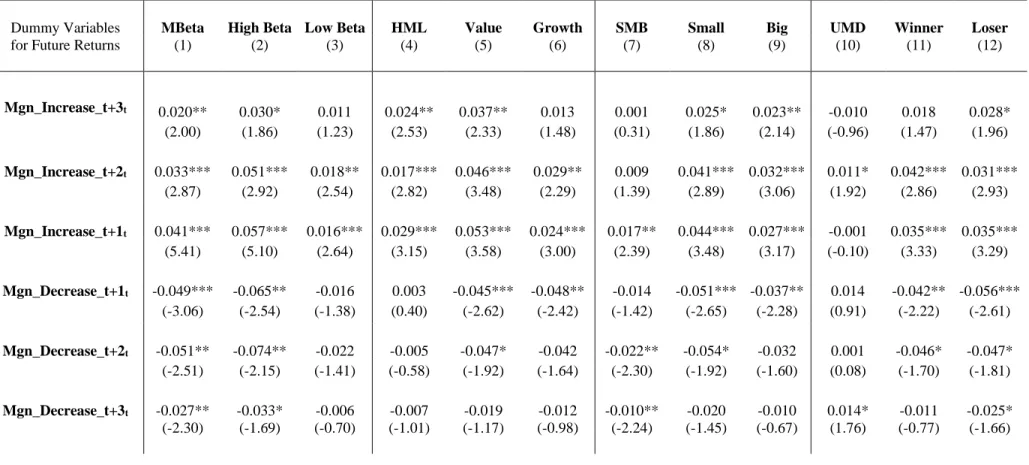
The results are provided in Table IV. Consider the coefficients of the six dummy
variables in the top half of Table IV, which reveal whether the return on each factor portfolio in month t rises (or drops) prior to increases (or decreases) in margin requirements over the next three months (t+1, t+2, or t+3). Consistent with the first prediction and the evidence in Figure 1, the return in month t on the first three factors (MBeta, HML, and SMB) reveals a positive
relation with anticipated future changes in margin requirements over the following three months. That is, these three hedge portfolio returns rise in the months before an increase in margin requirements and drop before a decrease in margin requirements. Moreover, these return
dynamics are driven by significant changes in returns on the riskier stocks in the long leg of each factor portfolio (i.e., high beta, value, and small stocks) prior to the change in margin
requirements. In contrast, the long and short legs of the momentum hedge portfolio behave similarly to each other in the months before increases or decreases in margin requirements. As a result, returns to the UMD hedge portfolio itself are largely unrelated to future margin changes. In the bottom half of Table IV, the coefficients of the control variables generally have the expected signs when significant. For example, the monthly returns on most portfolios are
inversely related to changes in the supply of margin credit, the price dividend ratio, and inflation. Together, the evidence in Table IV supports the first prediction, indicating that investors bid up (or down) the more risky stocks in the long legs of the first three factor hedge portfolios prior to increases (or decreases) in margin requirements, relative to the less risky stocks in the short legs. In contrast, these results suggest that investors do not similarly rely on the momentum factor to adjust their risk exposure in anticipation of future changes in leverage constraints.
18
In this subsection, we examine the second prediction of the theory of Black (1972) and Frazzini and Pedersen (2014) by estimating time series regressions that relate current or future returns on the factor portfolios to lagged margin requirements and the set of control variables. IV.B.1. Lagged Margin Requirements and One-Month-Ahead (Current) Returns
We begin by relating the current portfolio return in month t associated with each factor to lagged margin requirements in month t-1, the contemporaneous excess market return, and the other controls, as follows:
Ret_kt = α + β1 Margint-1 + β2 (Rm,t - Rf,t) + β3 ΔMgn_Creditt-1 + β4 Rm,t-12,t-1
+ β5 Rm,t-36,t-13 + β6 Volatilitym,t-12,t-1 + β7 Skewnessm,t-12,t-1
+ β8 Turnoverm,t-12,t-1 + β9 P/Dm,t-1 + β10ΔCPIt-13,t-1 + β11 ΔM1t-13,t-1
+ β12 ΔIPt-13,t-1 + εt . (2)
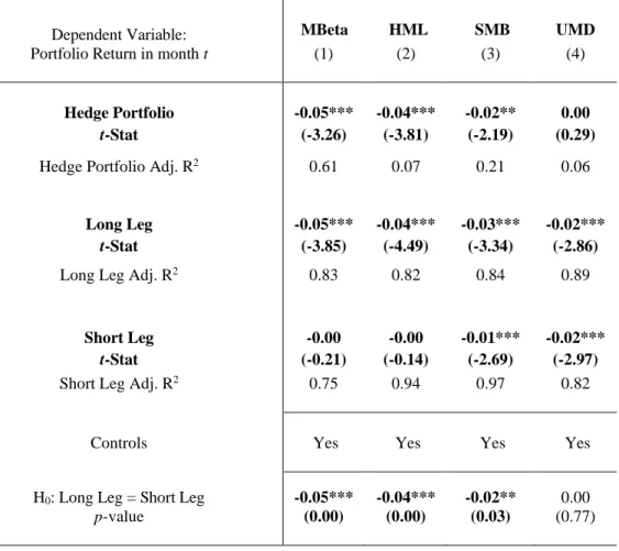
In Table V, we provide the coefficient of lagged margin requirements from this regression analysis for the four factor hedge portfolios (MBeta, HML, SMB, and UMD), as well as the long and short legs of each portfolio. The coefficients of the other control variables are generally similar to those provided in Table IV and are omitted here for brevity.
First, consider the top row of Table V, which provides the coefficient of lagged margin requirements from estimating Equation (2) for the MBeta, HML, SMB, and UMD hedge portfolios, respectively. Consistent with the second prediction and the evidence in Figure 1 and Table IV, the results indicate a significant negative relation between lagged margin requirements and subsequent one-month-ahead returns to hedge portfolios based on the first three factors (MBeta, HML, and SMB). That is, following an increase in margin requirements in month t-1, returns to the first three hedge portfolios are significantly lower in the following month. In contrast, returns to momentum (UMD) are unrelated to lagged margin requirements.
19
To understand the economic impact of this top row in Table V, consider the magnitudes of the changes in margin requirements during our sample period. Table I indicates that margin requirements were changed by +/- 10% seven times, by 15% 3 times, 20% six times, and 25% six times. In column (1) of Table V, the coefficient of lagged margin requirements is -0.05 (t-value = 3.26). This result implies that a 25% increase in margin requirements in month t-1 would be associated with a decline in the return on the MBeta hedge portfolio of 1.25% (= -0.05*.25) in the following month. For the HML or SMB factor in column (2) or (3) of Table V, the analogous coefficient of lagged margin requirements is -0.04 or -0.02 (t-value = -3.81 or -2.19), and the implied economic impact is a decline in the hedge portfolio return of 1.00% or 0.50% in the following month, respectively. In contrast, the coefficient of lagged margin requirements for UMD is 0.00 (t-value = 0.29). These results corroborate our preliminary findings in Figure 1, indicating that an increase (or decrease) in margin requirements in month t-1 is followed by a subsequent decline (or rise) in hedge portfolio returns based on the first three factors (MBeta, HML, and SMB), during the following month t. However, future returns to the momentum hedge portfolio are unaffected by changes in margin requirements.
Next we separately examine the long or short leg of each factor hedge portfolio. That is, we separately analyze high versus low beta stocks, value versus growth stocks, small versus big stocks, and winners versus losers. This separate analysis enables the data to distinguish between two potential alternative explanations for the negative relation we find in the top row of TableV – one that involves more risk-taking versus another that involves lessmispricing.
On the one hand, consistent with Frazzini and Pedersen (2014) and Jylha (2018), higher margin requirements may prompt investors to take more risk by overweighting high beta stocks, value stocks, or small stocks, leading to overvaluation of these riskier groups of assets. In this
20
scenario, an increase in margin requirements should have a stronger negative effect on the future returns to these subsets of riskier assets in the long legs of the first three factor hedge portfolios. On the other hand, higher margin requirements may instead limit the capital available to noise traders, making them less prone to buy the overpriced assets in the short legs of the HML and SMB factor portfolios (i.e., growth stocks and large stocks). In this case, an increase in margin requirements would mainly reduce the purchasing power of noise traders, and thereby decrease the overvaluation they cause in the short legs of the HML and SMB hedge portfolios.26
The results for the long and short legs of each factor portfolio appear in the second and third rows of Table V. For the first three factors (MBeta, HML, and SMB), the negative relation between margin requirements and future returns is concentrated among the riskier assets in the long leg of each hedge portfolio (i.e., high beta, value, and small stocks). The F-tests at the bottom of the first three columns in Table V verify that the differential effect of lagged margin requirements on one-month-ahead returns is significantly stronger for the riskier stocks in the long leg of these three factor portfolios. Together, this evidence is more consistent with a risk-based explanation for the negative relation between margin requirements and future returns on these three factor hedge portfolios. In contrast, this evidence does not support the alternative explanation based on reduced overpricing in the short leg, which would result from less buying by noise traders given higher margin requirements.
Finally, the evidence for momentum deviates from that for the other three factors. In particular, while the fourth column of Table V reveals a significant negative relation between lagged margin requirements and subsequent returns on each leg of the momentum factor (UMD),
26 Since individual investors rarely sell short, higher margin requirements should mainly curtail the buying of noise
traders, if it limits their trading at all (Barber and Odean, 2008, and Odean, 1999). In Section IV.B.2 below, we discuss an alternative scenario in which higher margin requirements may limit the capital available to arbitrageurs.
21
this negative relation is similar in magnitude for winners and losers. Indeed, the F-test at the bottom of column (4) indicates no significant difference between these coefficients for the long leg versus the short leg. As a result, there is no significant relation between margin requirements and future returns to the combined UMD hedge portfolio itself.
IV.B.2. Lagged Margin Requirements and Longer-Term Future Returns
In this section, we consider another potential alternative explanation for our findings that returns to the first three factor hedge portfolios are significantly lower in the short run, following an increase in margin requirements. According to this alternative explanation, higher margin requirements may limit the capital available to arbitrageurs, which prevents them from correcting the mispricing or even allows noise traders to temporarily exacerbate this mispricing (e.g., see
Campbell and Kyle, 1993, and De Long, Shleifer, Summers, and Waldman, 1990). If the prices of stocks in the long and short legs of the factor portfolios deviate further from fundamentals in the short run after an increase in margin requirements, for this reason, this deviation could lead to negative returns for the factor hedge portfolios that is not corrected by arbitrageurs.
We note that this alternative explanation is not consistent with our evidence of higher
(lower) hedge portfolio returns for MBeta, HML, and SMB prior to future increases (decreases)
in margin requirements. Furthermore, an additional implication of this alternative explanation is that, in the longer run after an increase in margin requirements, prices should ultimately
converge back toward fundamentals, so that we should eventually observe a reversal from a negative relation to a positive relation. We test this additional implication by examining the relation between margin requirements and longer run future returns on each factor, for up to
twenty-four months following the change in margin requirements in month t-1. This analysis
22
hedge portfolios constructed in month t. However, the factors in Kenneth French’s data library
(HML, SMB, and UMD) are updated only annually, and the underlying stocks are unknown to us. Thus, it is not possible to calculate future returns on a monthly basis over longer horizons, for the same set of stocks in each Fama-French factor.
We overcome this problem by constructing our own replicating hedge portfolios each
month for the HML, SMB, and UMD factors. These replicating portfolios are necessary for our
analysis of longer-term future returns for the portfolios of stocks in each factor portfolio, as well as the long and short legs of each hedge portfolio, around changes in margin requirements. We follow Davis, Fama, and French (2000) to calculate the replicating portfolios for the HML and SMB factors. In particular, we use sorts based on the book to market data provided on Kenneth French’s website to construct our own replicating portfolio for the HML factor, and we use the firm’s market capitalization to construct our own SMB factor. We create the replicating hedge
portfolio for momentum by ranking stocks each month (t) into deciles based on their cumulative
stock returns over the prior twelve months, t-13 to t-2. We then form the UMD hedge portfolio
that is long past winners (highest decile) and short past losers (lowest decile) in month t-1, and
we compute the future return to this UMD portfolio for the next twenty-four months, t to t+23.
We begin by examining whether our replicating factor portfolios display similar behavior to the three Fama and French (1993) factors from Kenneth French’s web site. The correlations between the monthly returns on our three replicating portfolios and the associated Fama and French factors (HML, SMB, and UMD) are 0.93, 0.87, and 0.85, respectively. This outcome suggests that we can extend inferences from our own replicating factor portfolios to the factor portfolios of Fama and French.
23
We next relate the longer run future returns on these replicating factor hedge portfolios to lagged margin requirements, as follows:
Ret_kt+i, t+j = α + β1 Margint-1 + Controls + εt . (3)
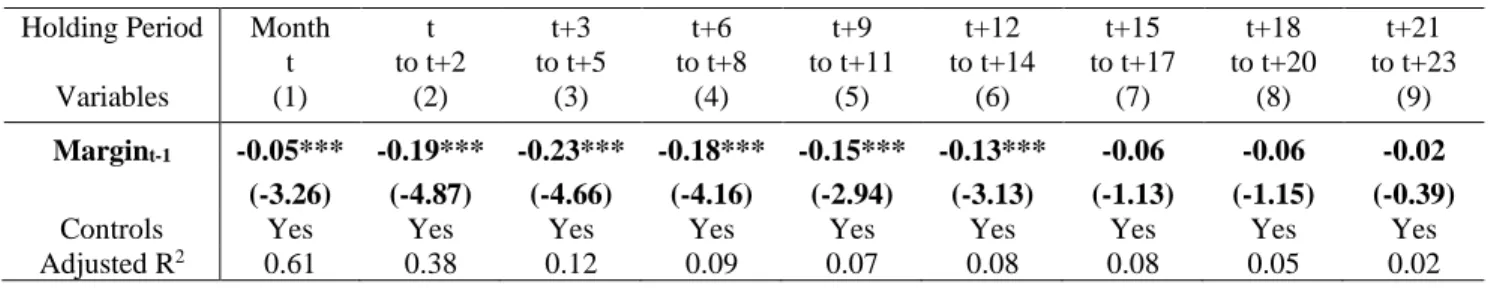
Now the dependent variable is the longer run future return to each replicating factor hedge portfolio, as described above (k = MBeta, HML, SMB, or UMD). First, as before, we hold every replicating hedge portfolio for one month (t) following the change in margin requirements in month t-1. In addition, we hold each hedge portfolio over a series of future three-month periods that span the next twenty-four months, from month t to t+2, t+3 to t+5, t+6 to t+8, t+9 to t+11, t+12 to t+14, t+15 to t+17, t+18 to t+20, and t+21 to t+23. The resulting hedge portfolio return for every future three-month period (Ret_kt+i, t+j) is then regressed on lagged margin requirements
in month t-1 and the controls from Equation (2), which are defined in Table II.
In Panel A of Table VI, we provide the results of estimating Equation (2) and Equation (3) for the MBeta hedge portfolio. In Panels B, C, and D, we present the analogous evidence for HML, SMB and UMD, respectively. As expected, column (1) of each Panel reveals that the results for short run (one-month-ahead) future returns to all four replicating factor hedge portfolios are similar to the analogous evidence for the original Fama and French portfolios, provided in Table V above.
Next, we turn to the evidence for longer run future hedge portfolio returns in columns (2) to (9) of Table VI. This evidence indicates that the significant negative relation between lagged margin requirements and one-month-ahead returns for the first three factor portfolios (MBeta, HML, and SMB), in column (1), continues to prevail over each successive three-month period that spans the following 12 to 21 months, before becoming insignificant near the end of this 24-month period. Once again, the evidence for momentum deviates from the other three factors in
24
Table VI, since the longer-term future returns to momentum (UMD) are never significantly negatively related to past margin requirements throughout the next 24 months.
It is important to emphasize that, for the first three factor portfolios, there is no eventual reversal of this short run negative relation to a longer-term positive relation between margin requirements and future returns. This outcome does not support the alternative explanation based on a temporary divergence of prices further from fundamentals, due to limited capital available to arbitrageurs. Instead this evidence is more consistent with the second prediction from the theory of Black (1972) and Frazzini and Pedersen (2014).
V. Margin Requirements and the SML Analogues from Multifactor Models
In this section we examine the association between margin requirements and time series variation in the monthly intercept and slope coefficients of the SML analogues implied by the Fama-French (1993) three-factor model or the Carhart (1997) four-factor model. We measure this association using a two-stage analysis. In the first stage, each month (t) we begin by estimating the sensitivity of returns on a set of test assets to every factor over the previous 36 months. We then estimate the cross-sectional relation between the returns on these test assets and their respective estimated factor sensitivities in month t, to obtain the monthly intercept and slopes of the SML analogues for all factors. In the second stage, we estimate the time series relation between each monthly intercept or slope coefficient and lagged margin requirements, along with our set of control variables. We next discuss each stage of this analysis, in turn.
V.A. First Stage: Estimating Factor Sensitivities and the Intercept and Slopes of SML Analogues In our first stage, we follow Cohen, Polk, and Vuolteenaho (2005) and Jylha (2018), who estimate the intercept and slope of the CAPM security market line. In Jylha (2018), stocks are first grouped each month (t) into twenty value-weighted portfolios based on their historical betas,
25
estimated with rolling regressions of excess stock returns on excess market returns over the previous 36 months. Next, each month (t) the value-weighted returns of each portfolio are
regressed on excess market returns (the first factor) over the prior 36 months to obtain its ex-ante beta. Then, each month (t) the cross section of realized returns on these twenty portfolios of test assets are regressed on their ex-ante betas. The resulting monthly intercept and slope of the CAPM security market line are retrieved from this last regression.
We employ similar methodology, with an expanded approach that enables us to obtain the monthly intercept and slopes for the SML analogues corresponding to all factors included in either the three-factor model or the four-factor model. We wish to analyze test assets that vary along all dimensions embodied in either multifactor model. We therefore begin by stratifying the set of all NYSE stocks each month (t) according to the three factors in the Fama and French (1993) model, or the four factors in the Carhart (1997) model, respectively, in order to generate portfolios of test assets that vary along each dimension analyzed.
Consider our analysis of the Fama and French (1993) three-factor model. Here we wish to analyze test assets that vary along the three dimensions: beta, book-to-market, and size. Thus, we independently sort stocks into four groups every month (t) based on each of the three
dimensions: (i) the stock’s historical market beta estimated over months t-36 to t-1, (ii) book-to-market ratio for the prior fiscal year, and (iii) firm size in month t-1. This 4 × 4 × 4 sorting scheme generates a set of 64 portfolios of test assets each month (t), stratified along all three dimensions. The value-weighted returns for each portfolio of test assets are then regressed on each of the three factors over the previous 36 months (t-36 to t-1), to retrieve the ex-ante
sensitivity of each portfolio’s return to the market, HML, and SMB factors, respectively. Finally, the cross section of value-weighted excess returns to these 64 portfolios in month t are regressed
26
on their three ex-ante sensitivities estimated above. This last regression yields the monthly intercept and slope coefficients for the SML analogues implied by the three-factor model.27 V.B. Second Stage: Relating Intercepts and Slopes of SML Analogues to Margin Requirements
In the second stage, we regress the monthly intercept or each slope coefficient from the SML analogues against lagged margin requirements and the controls defined above, as follows:
Interceptt = α1 + β1 Margint-1 + Controls + ε1t , (4)
Slope_kt = α2 + β2 Margint-1 + Controls + ε2t , (5)
where Intercept is the intercept, and Slope_k is the slope coefficient for the SML analogue associated with each factor estimated in month t, implied by the three-factor or four-factor model (i.e., k = the market return, HML, SMB, or UMD). All variables are defined in Table II.
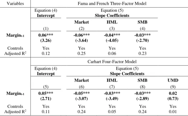
In Table VII, we present the results for each second stage regression estimated. Columns (1) to (4) in Panel A present the analysis for the monthly time series regressions based on the intercept and slope coefficients from the three-factor model (including the market, HML, and SMB). Columns (1) to (5) in Panel B present the analogous results for the four-factor model (including the market, HML, SMB, and UMD). Robust t-ratios are provided in parentheses. In Panels A and B of Table VII, the monthly intercepts from the three-factor and four-factor models both reveal a significant positive relation with lagged margin requirements. This positive relation suggests that these multifactor models fail to adequately explain the variation in the performance of the test assets analyzed when margin requirements are varied. On the other
27 Our analysis of the Carhart (1997) four-factor model is similar. Here, each month we independently sort NYSE
stocks into three groups based on each of the four factors: (i) beta, (ii) book-to-market, (iii) size, and (iv) momentum returns over the past twelve months. This 3 × 3 × 3 × 3 sorting scheme generates 81 portfolios of test assets each month. The value-weighted returns to each of these 81 portfolios are then regressed on each of the four factors over the prior 36 months, to retrieve the 81 sensitivities to each of these four factors. Finally, the cross section of
value-weighted excess returns to these 81 portfolios in month t are regressed on their four ex-ante sensitivities estimated
27
hand, the slope coefficients for the first three factors (i.e., the market, HML, and SMB) are negatively related to margin requirements. This evidence is consistent with the second prediction of Black (1972) and Frazzini and Pedersen (2014), indicating that tighter leverage constraints result in flatter SML analogues for the market, HML, and SMB factors, which implies lower subsequent compensation for these aspects of risk. In contrast, there is no significant relation between margin requirements and the slope of the fourth momentum factor (UMD) in Panel B.
To understand the economic significance of these results, consider the implications of a 25% change in margin requirements for the intercept or slope coefficient that pertains to each factor. For example, in columns (1) to (4) of Panel A in Table VII, the coefficient of lagged margin requirements is 0.02 (t-ratio = 1.8) for the regression involving the intercept, and is -0.03 (with t-ratios that range from -2.5 to -3.2) for the regressions involving the three factors (i.e., the market, HML, and SMB). This evidence indicates that a 25% increase in margin requirements in month t would be associated with an average increase in the alpha of the three-factor model in month t+1 by 50 basis points (i.e., 0.02 × 0.25), and an average decline in the slope of each SML analogue by 75 basis points (i.e., -0.03 × 0.25).
VI. Extensions and Robustness Tests
In this section, we examine the robustness of our main results when we analyze alternative test assets or consider additional control variables.
VI.A. Alternative Test Assets
In this subsection, we repeat the analysis from Table VII using two alternative sets of test assets. We generate the first set of alternative test assets by conducting a two-way 5 × 5 sorting scheme each month (t), in which we independently partition the set of all NYSE stocks into five groups based on just the two firm attributes, book-to-market and size, to form 25 value-weighted
28
portfolios. Our second alternative set of test assets includes the Fama and French 49 industry portfolios each month (t), which are available from the Kenneth French data library. In the latter analysis, we exclude the eight industries that have missing observations sometime during our sample period, which leaves 41 industries with a complete return history.28
For each alternative set of test assets, we follow the same two-stage regression analysis to retrieve the monthly intercept and slopes of the SML analogues for each factor, and then estimate the relation between lagged margin requirements and each intercept or slope coefficient. In Panel A (B) of Table VIII, we provide the results from estimating Equation (4) and Equation (5) using the first (second) alternative set of test assets. In columns (1) to (4) of each Panel, we present the results for the intercept and SML slope coefficients based on the three-factor model. In columns (5) to (9), we provide the analogous results for the four-factor model.
The results in both Panels of Table VIII are similar to the evidence in Table VII. In particular, the monthly intercept from each multifactor model is again positively related to margin requirements, while the SML slope coefficients for the first three factors (i.e., the market, HML, and SMB) are negatively related to margin requirements. In contrast, the slope of the fourth momentum factor (UMD) is unrelated to margin requirements. This analysis shows that our main results for Equation (4) and Equation (5) are robust when we base the analysis on alternative test assets each month.
VI.B. Market Neutral Factor Portfolios
Our explanation for the negative relations between lagged margin requirements and the slope coefficients for the SML analogues pertaining to the HML and SMB factors implies that
28 Results are robust when we exclude just the missing observations each month (t), instead of excluding all
observations from the eight industries that have some missing observations. Results are also robust when we analyze the Fama and French 30 or 48 industry portfolios.
29
these two hedge portfolios capture aspects of risk that differ from the market beta. However, Liu (2018) notes that the hedge portfolio returns associated with many asset pricing anomalies reveal a negative sensitivity to the market portfolio (i.e., they have a negative market beta). As a result, hedge portfolio returns associated with many anomaly variables mechanically incorporate the betting-against-beta anomaly of Frazzini and Pedersen (2014). According to Liu (2018), it is the betting-against-beta anomaly that drives the returns to many anomalies, rather than any true anomalous predictive relation associated with those anomaly variables.
While Liu (2018) does not examine the book-to-market and firm size anomalies that are associated with HML and SMB in our analysis, we find that the correlations of Mbeta with HML
and SMB are significantly positive (at 0.40 and 0.66, respectively).29 These high correlations
may reflect a tendency for value stocks and small stocks to have higher market betas, making our analysis susceptible to a critique similar to that in Liu (2018). That is, this high correlation suggests that our results may be driven by a failure to control for the influence of market beta on HML and SMB, rather than by investors’ response to more binding leverage constraints.
We address this issue by constructing new replicating portfolios for HML, SMB, and UMD that are neutral with respect to the market (i.e., that have zero market betas), and repeating our main analysis using these market-neutral factor portfolios. We construct these market-neutral factor portfolios using a methodology similar to Liu (2018) by eliminating high (low) beta stocks from the long (short) legs of the HML and SMB factors, respectively. For example, for the HML factor we eliminate high beta stocks from the value portfolio and low beta stocks from the growth portfolio. In particular, we examine a subset of the value stock portfolio (the long leg of HML), by retaining only stocks that are below the 70th percentile in terms of their market beta,
30
and higher than the 70th percentile in terms of their book-to-market ratio. Similarly, we retain a subset of the growth stock portfolio (the short leg of HML) that are above the 30th percentile in terms of their market beta, and below the 30th percentile in terms of their book-to-market ratio.
We follow a similar approach for the long and short legs of the SMB and UMD factors.30
The correlation between MBeta and our market-neutral factor portfolios (labeled N-HML, N-SMB, and N-UMD) are 0.03, -0.018, -0.206, respectively. Hence, this method yields N-HML and N-SMB portfolios that are indeed market-neutral, since they have zero correlation with the MBeta portfolio. In addition, this method produces a portfolio for momentum (N-UMD) that has a smaller negative correlation with the MBeta portfolio.
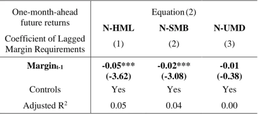
Next, we repeat our analyses from Table V and Table VII using these market-neutral portfolios, N-HML, N-SMB, and N-UMD. The evidence for future one-month-ahead returns to these market-neutral hedge portfolios is presented in Panel A of Table IX, while the evidence for the intercepts and slopes of the SML analogues for the three- and four-factor models appears in Panel B. The main results and conclusions are unchanged. In Panel A, lagged margin
requirements are negatively related to subsequent returns on the market-neutral factor portfolios, N-HML and N-SMB, while they are unrelated to future returns on the market-neutral N-UMD
factor portfolio.31 Similarly, in Panel B, margin requirements are once again positively related to
the intercept and negatively related to the slopes of the first two market-neutral factors, N-HML
and N-SMB, while they are unrelated to the slope of the N-UMD factor. We conclude that our
30Since UMD has a negative correlation with MBeta, we eliminate low (high) beta stocks from the long (short) legs of the UMD factor.
31 In untabulated results, we find that the negative relation between margin requirements and one-month-ahead
returns to the first two market neutral factor portfolios, N-HML and N-SMB, documented in Table IX, also extends further into the future when we examine longer term future returns, similar to the results in Table VI.
31
results are robust when we control for the sensitivity of the HML, SMB, and UMD factors to market beta, and therefore our conclusions are not subject to the critique of Liu (2018).
VI.C. Controlling for the Cost of Leverage for Investors
In this subsection, we repeat the analysis from Tables V and VII, but we also control for investors’ cost of leverage. When lending and borrowing rates differ, efficient portfolios that involve borrowing lie on a flatter line than the alternative set of efficient portfolios that involve lending. Thus, in addition to restrictions on borrowing, another potential market friction that could lead to a flatter relation between expected returns and return sensitivities (i.e., a flatter SML analogue) for various risk factors is the difference between borrowing and lending rates.
Here we expand Equations (2), (4), and (5) to include a proxy for the difference between borrowing and lending rates, or investors’ cost of leverage. Our proxy is the call spread, defined as the difference between the broker’s call money rate and the three-month Treasury Bill rate. Theoretically, a higher call spread could be associated with a flatter SML analogue for each factor. As a result, the call spread may be positively related to the intercept and negatively related to the slope coefficient for each factor.32
In Table X, we present this expanded analysis of Equations (2), (4) and (5). For every regression, we present the evidence for two specifications that include the lagged call spread, with and without lagged margin requirements. For brevity, we only present the coefficients for our two main variables of interest, lagged margin requirements and the call spread.
In Panels A and B of Table X, we estimate the expanded version of Equation (2), to analyze returns on the long leg and the short leg of each factor portfolio, as well as the hedge portfolio itself. In Panel A we provide the results for MBeta and HML, while Panel B presents the
32
results for SMB and UMD. Similar to the evidence in Table V, the results indicate a significant negative relation between lagged margin requirements and the monthly return to the first three factors, which is driven by the riskier stocks in the long leg of each factor hedge portfolio. In contrast, lagged margin requirements are again unrelated to returns on momentum (UMD).
In Panels C and D of Table X, we present the analogous results from estimating a
similarly expanded version of Equation (4) and Equation (5) in the second stage of our analysis of the SML intercept and slope coefficients. In Panel C, we provide the results for the Fama and French (1993) three-factor model, and in Panel D we present the results for the Carhart (1997) four-factor model. Once again, including the lagged call spread in the model does not alter the coefficient of lagged margin requirements from Table VII, which remains significantly positive in regressions involving the intercept, and significantly negative in regressions involving the first three factors of each model (i.e., the market, HML, and SMB). In contrast, there is again no significant relation between lagged margin requirements and the SML slope analogue for the momentum factor (UMD).
Throughout all specifications in Panels A – D of Table X, the coefficient of the lagged call spread is never significantly different from zero. Furthermore, this coefficient does not change substantially when we add lagged margin requirements to the model. This evidence indicates that our results from Tables V and VII are not driven by investors’ cost of leverage, or by some unspecified association between margin requirements and this cost of leverage.
VI.D. Disagreement,Short Sale Constraints, and Margin Requirements
Hong and Sraer (2016) examine the influence of investor disagreement and short sale constraints on the slope of the CAPM security market line. They argue that, when investors disagree about prospects for the macroeconomy, assets with a high market beta are more