A Methodology for Optimizing
Statistical Multi-Response Problems
Using Fuzzy Goal Programming
M. Amiri
and J. Salehi-Sadaghiani
1This paper presents a method for optimizing statistical multi-response problems. The method is based on fuzzy goal programming and it enjoys a strong mathematical foundation. In this method, the decision maker's comments are considered objectively. The LINGO programming environment is used to test the developed method. The method performance is evaluated by comparing the results with those of other existing methods.
INTRODUCTION
In multi objective decision making environments, a problem of interest is to select a set of input conditions (or independent variables), which results in a product with a desirable set of outputs (or response variables). In fact, this problem is about simultaneous optimiza-tion of the response variables, Y1; ; Ym, each of
which depends upon a set of independent variables, X1; ; Xn. Here, it is desirable to select the levels
of the independent variables such that all the response variables are optimized [1].
For example, as mentioned in [1], in quality control environments, the goal may be to nd the levels of the input variables (quality characteristics) of the process, so that the quality of the product has the desired characteristics. Also, in Response Surface Methodology (RSM), the levels of the input variables are adjusted until the set of outputs are optimized.
Since goods have more than one qualitative at-tribute, the simultaneous improvement of these quali-tative attributes is very important. A common problem in the simultaneous optimization of multi-response problems is that optimizing one attribute aects the other qualitative attributes. In other words, a set of conditions which is optimized for one attribute is not necessarily optimized for other attributes. Therefore, designing a method, which can oer an acceptable
*. Corresponding Author, Department of Industrial Man-agement, Allame Tabataba'ee University, Tehran, I.R. Iran. E-mail: mg [email protected]
1. Department of Industrial Management, Allame Tabataba'ee University, Tehran, I.R. Iran.
product considering dierent aspects is important [2]. Multi-response optimization in the framework of RSM is an attempt to reach this end.
Classic methods, such as bounded objectives or a combination of bounded objectives and lexicography, are used in multi-response optimization. Myers and Carter used the method of bounded objectives for the rst time and they proposed optimizing the main solution [3]. Biles extended this method for more than two solutions [4]. Myers, Khari and Vining extended these results by combining Myers and Carter's method with Taguchi's method. They used deviation and response eects as two independent solutions in their optimization [5].
The loss function method was used by Tang and Lo [6], Pignatello [7], Winston [8], Artiles-Leon and Ross [9,10], Kapur and Cho [11] and Robert and Richard [12]. The basis of this method is Taguchi's loss function, in which a second order loss function, encompassing qualitative attributes and, in some cases, qualitative attributes variance, is oered. Taguchi's loss function is a second order function of the deviation of the desirable qualitative attribute from the target value, as shown by Relation 1:
Loss(Y (X)) = k(Y (X) T ): (1)
In Relation 1, k is the loss coecient factor and T is the desired value of the qualitative attribute. Extending Taguchi's loss function, Artiles-Leon oered the loss function shown by Equation 2:
L(Y; X; T ) = 4Xk
i=1
Yi(X) Ti
USLi LSLi
2
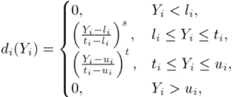
Derringer and Suich [13] introduced a useful class of desirability functions. There are two types of transfor-mation from Yi to di(Yi), namely, one-sided and
two-sided. The one-sided transformation is applied when Yi
is to be maximized and the two-sided transformation is used when Yi is to be assigned a target value.
In a two sided transformation, assume li and ui
to be the lower and upper limits of the response, Yi,
respectively. Also, assume that ti be the target value
of the response, Yi, respectively, such that li< ti< ui.
The desirability function is dened by the following equation:
di(Yi) =
8 > > > > > < > > > > > :
0; Yi< li;
Yi li
ti li
s
; li Yi ti;
Yi ui
ti ui
t
; ti Yi ui;
0; Yi> ui;
(3)
In Equation 3, the exponents, s and t, determine how strictly the target value is desired and the user must specify their values [1]. Derringer and Suich oered Relation 4 for computing the decision function:
D(Y ) = [d1(Y1):d2(Y2) dk(Yk)]1=k: (4)
Zimmermann oered a method for solving multi-objective linear programming problems using fuzzy logic [14]. Later, Cheng and his colleagues extended the Zimmermann method for optimizing statistical multi-response problems [15]. Keeny and Raia presented a method for multiple objective problems using prefer-ences and value tradeos [16].
Noorossana and his colleagues oered a method for extracting and using the decision function in opti-mizing multi-response problems [17] and Pasandideh and Niaki [1] modeled a multi-response statistical optimization problem through the desirability function approach, where they applied four GA methods to solve this model by simulation. They also studied the performance of each method through dierent simulation replications and statistically compared them via a performance measure.
The solutions of most of the above existing meth-ods take a long time to generate. This weakness is due to the rapid increase in solution time, as the number of qualitative attributes and objectives increase. For
this reason, designing optimization algorithms for sta-tistical multi-response problems that do not have this disadvantage is of special importance.
In this paper, a methodology for optimizing statistical multi-response problems, using fuzzy goal programming, is presented. Through some examples, the desirable execution time of the developed algorithm will be shown when the number of factors and/or objectives increase. The paper is organized as follows: First, denitions are presented. Next, the model and the proposed methodology are explained and numerical examples and comparison with other existing methods will, subsequently, be shown. Finally, the conclusion and the nomenclature are given.
DEFINITION 1
The mathematical model of the multiobjective problem is dened as follows:
max Zj = Yj(X1; X2; ; Xn); j = 1; 2; ; m
1 Xj 1; j = 1; 2; ; n:
DEFINITION 2
If, in a multi objective problem with m objectives, each objective function is solved independently, then, one has m independent optimal solutions. By replacing each optimal solution in the other objective functions, a lower and upper limit for each objective function will be gained.
For the ith objective function, the following prob-lem is solved separately (i = 1; 2; ; m). The results are shown in Table 1, in which Zij is the value of the
jth objective function, in terms of optimal variables of the ith objective function problem; Xij is the optimal
value of variable Xj in the ith objective function.
DEFINITION 3
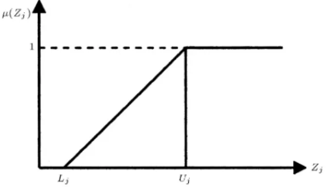
For any objective function, there is a fuzzy membership function (shown in Figure 1) as follows:
(Zj) =
8 > < > :
0 Zj< Uj j = Lj Zj (Uj j)
j Uj j Zj Uj
1 Zj Uj
(5)
Table 1. The range of objective functions.
Z1 Z2 Zm X1 X2 Xn
max(Z1) Z11= Z1 Z12 Z1m X11 X12 X1n
max(Z2) Z21= Z1 Z22= Z2 Z2m X21 X22 X2n
..
. ... ...
Figure 1. Membership function of Zj function. where:
Uj = Zj; Lj = mini (Zij); j= Uj Lj:
THE MODEL AND THE PROPOSED METHODOLOGY
In this paper, the following assumptions are made: 1. All the factors that make up the input of the
prob-lem, are the independent variables X1; X2; ; Xn;
2. The lower and upper bounds of the independent variables are -1 and 1, where Xj is a coded variable,
such that 1 Xj 1;
3. The output of the problem is the response variables denoted by Y1; Y2; ; Yk;
4. For every objective function Zj, one has:
Lj Zj Uj:
5. The one-sided or two-sided transformation for each response depends on the nature of the objective of the problem.
The mathematical model of the problem becomes: max : Zj = Yj(X1; X2; ; Xn);
j = 1; 2; ; m; s.t:
1 Xj 1; j = 1; 2; ; n:
Theorem 1
Consider the following response variable problems: max : Zj = Yj(X1; X2; ; Xn);
j = 1; 2; ; m; s.t:
1 Xj 1; j = 1; 2; ; n:
Assuming an identical importance for the objectives and an identical access level to the optimal point of each objective, the decision maker's desirable solution is found by solving the following mathematical pro-gramming model:
max : ; s.t:
Zj
j + nj pj=
Uj
j; j = 1; 2; ; m;
+ nj 1; j = 1; 2; ; m;
1 Xj 1; j = 1; 2; ; n;
20 1;
nj 0; pj 0; j = 1; 2; ; m; (6)
where:
pj: the function positive deviation, Zj=j,
nj: the function negative deviation, Zj=j,
: access level to the optimum of any objective function.
Proof
In Figure 1 there is: (Zj) =
8 > < > :
0 Zj< Uj j = Lj Zj (Uj j)
j Uj j Zj Uj
1 Uj Zj
; = min
j (Zj) ) max : ;
(a)
Zj
j
Uj
j + 1;
Uj
j 1
Zj
j
Uj
j;
for some j (nj: negative deviation);
(b) Uj
j
Zj
j
Uj
j + 1; for some j:
For the constraints of section (a), suppose that: Zj
j =
Uj
j nj:
Now, one has: + nj 1; Zj
j + nj=
Uj
For the constraints of section (b), suppose that: Zj
j = pj+
Uj
j; (pj : positive deviation):
Now, one has: Zj
j pj=
Uj
j: (8)
Now, Constraints 8 and 9 are combined and, nally: max :
Zj
j + nj pj =
Uj
j; j = 1; 2; ; m;
+ nj 1; j = 1; 2; ; m;
1 Xj 1; j = 1; 2; ; n;
20 1; nj 0; pj 0; j = 1; 2; ; m:
Corollary 1
If the access level to the optimum state of each objec-tive is dierent and the objecobjec-tives are not identically important from the viewpoint of the decision maker, then, the desirable solution of the decision maker is obtained by solving the following mathematical model:
max :Xm
j=1
Wjj;
Zj
j + nj pj =
Uj
j;
j+ nj 1;
1 Xj 1;
j 2 0 1;
nj 0; pj 0: (9)
Proof
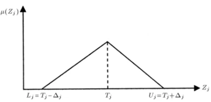
This is the result of Theorem 1, with the following assumptions (shown in Figure 2):
j (Zj):
Figure 2. Membership function of Zjobjective function. Corollary 2
If the response variables have the best nominal value (two-sided transformation), the objectives are not iden-tically important from the view point of the decision maker and the access level to the optimum status of each objective is dierent, then, the decision maker's desirable solution is obtained by solving the following mathematical model:
max :Xm
j=1
Wjj;
Zj
j + nj pj =
Tj
j;
j+ nj+ pj 1;
1 Xj 1;
j 20 1; pj 0; nj 0; (10)
where Tj is nominal value of objective function Zj.
Proof
This is the result of Theorem 1 with the following assumptions:
(Zj) =
8 > > > > < > > > > :
0 Zj< Tj j
Zj (Tj j)
j Tj j Zj< Tj
Tj+j Zj
j T Zj < Tj+ j
0 Zj Tj+ j
j (Zj): (11)
Corollary 3
If there are k response variables on \the more { the better" (one-sided transformation), the m k response variables are on the better nominal value (two-sided transformation) and the goals are not identically im-portant from the viewpoint of the decision maker, then, the desired solution, from the viewpoint of the decision
maker, is obtained by the following mathematical model:
max :Xm
j=1
Wjj
Zj
j + nj Pj=
Uj
j; j = 1; 2; ; k;
Zj
j + nj Pj=
Tj
j; j = k + 1; k + 2; ; m;
j+ nj 1; j = 1; 2; ; k;
j+ nj+ pj 1; j = k + 1; k + 2; ; m;
1 Xj 1; j = 1; 2; ; n;
j 20 1;
nj 0; pj 0: (12)
The proof is obtained from Corollaries 1 and 2. Based on the proof of this theorem, an algorithmic procedure for calculating the response surface is now proposed.
Algorithm
Step 1: Dene the following response variable prob-lems:
max : Zj= Yj(X1; X2; ; Xn);
j = 1; 2; ; k
min : rj = Rj(X1; X2; ; Xn);
j = k + 1; k + 2; ; m;
s.t : 1 Xj 1; j = 1; 2; ; n:
Step 2: Change the response variable problems as fol-lows:
max : Zj= Yj(X1; X2; : Xn);
j = 1; 2; ; m;
s.t : 1 Xj 1; j = 1; 2; ; n:
Step 3: Solve the problem for each objective function separately and obtain the solutions. Put the solutions in the objective functions. For each objective function obtain two lower limit (Lj)
and upper limit (Uj) as the best and the worst
case and, then, obtain j = Uj Lj.
Step 4: Obtain the objective weights, Wj, from the
decision maker and then solve the following mathematical programming model:
max :
m
X
j=1
Wjj;
Zj
j + nj Pj =
Uj
j; j = 1; 2; ; m;
j+ nj 1; j = 1; 2; ; m;
1 Xj 1; j = 1; 2; ; n;
j20 1; j = 1; 2; ; m;
pj 0; nj 0; j = 1; 2; ; m:
NUMERICAL EXAMPLES AND COMPARISON
Example 1
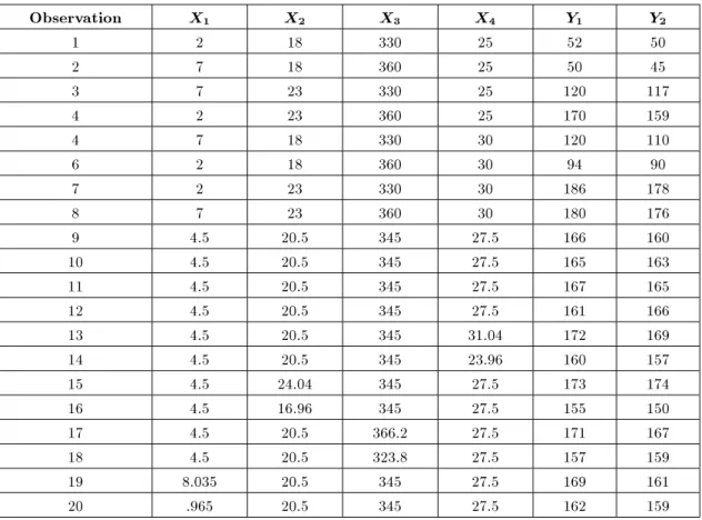
This example concerns research that has been done by Noorossana [17] and has four design variables: The ammoniac (X1), the thickness of lead and expulsion
alloys on the radiator pipe X2), the temperature (X3)
and the percentage of expulsion in the alloy of the radiator pipe (X4).
The responses are corrosion (Y1) and adhesiveness
(Y2). The design is a central composite design. The
data are given in Table 2.
The correlation coecient and covariance matrix of the responses Y1; Y2are as follows:
R Y1; Y2= 0:994;
S2 Y
1; Y2=
1580:79 1582:55 1582:55 1599:04
:
Therefore, the responses, Y1 and Y2, are highly
corre-lated. At rst, the above data was coded. Then, a second-order model was tted for both responses. The response surface curves for Y1 and Y2are as follows:
Y1= 250:34 34:26X1+ 43:91X2 1:55X3
+ 6:75X4 22:97X22 21:84X32 23:22X42
+ 4:56X1X4+ 16:94X2X4+ 25:31X3X4; (13)
Y2=176:75 2:01X1+30:6X2+2:59X3+16:87X4
13:31X2
1 13:19X22 12:94X32 12:44X42
Table 2. Experimental data.
Observation X1 X2 X3 X4 Y1 Y2
1 2 18 330 25 52 50
2 7 18 360 25 50 45
3 7 23 330 25 120 117
4 2 23 360 25 170 159
4 7 18 330 30 120 110
6 2 18 360 30 94 90
7 2 23 330 30 186 178
8 7 23 360 30 180 176
9 4.5 20.5 345 27.5 166 160
10 4.5 20.5 345 27.5 165 163
11 4.5 20.5 345 27.5 167 165
12 4.5 20.5 345 27.5 161 166
13 4.5 20.5 345 31.04 172 169
14 4.5 20.5 345 23.96 160 157
15 4.5 24.04 345 27.5 173 174
16 4.5 16.96 345 27.5 155 150
17 4.5 20.5 366.2 27.5 171 167
18 4.5 20.5 323.8 27.5 157 159
19 8.035 20.5 345 27.5 169 161
20 .965 20.5 345 27.5 162 159
The studied multi-response problem is as follows: max : Z1= Y1; max : Z2= Y2;
s.t:
1 Xj 1; j = 1; 2; 3; 4: (15)
Proposed Method
First, the two problems are solved independently: max : Z1= Y1;
s.t:
1 Xj 1; j = 1; 2; 3; 4; Z2= Y2;
max : Z2= Y2;
s.t:
1 Xj 1; j = 1; 2; 3; 4; Z1= Y1: (16)
The results are shown in Table 3. Now, one has: 1= 311 272 = 39; U1= 311;
2= 198 180 = 18; U2= 198:
Then, the following problem is solved: max : W11+ W22
Zi
i + ni pi=
Ui
i; i = 1; 2;
ni+ i 1; i = 1; 2;
ni 0; pi 0; i20 1; i = 1; 2: (17)
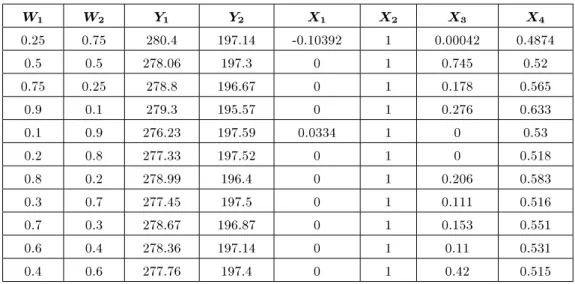
The sensitivity analysis on W1 and W2 is shown in
Table 4.
By increasing Wi, the value of Yi would be
increased. As is clear, the best solution is obtained by considering W1= 0:25 and W2= 0:75.
The three foregoing problems were solved using LINGO software. Based on this example, the compar-ison between the proposed method and existing ones are shown in Table 5.
The above example was presented to evaluate the
Table 3. The range of objective functions.
Z1 Z2 X1 X2 X3 X4
max(Z1) 311 180 -1 1 0.297 0.574
Table 4. The range of objective functions for dierent values of W1and W2.
W1 W2 Y1 Y2 X1 X2 X3 X4
0.25 0.75 280.4 197.14 -0.10392 1 0.00042 0.4874
0.5 0.5 278.06 197.3 0 1 0.745 0.52
0.75 0.25 278.8 196.67 0 1 0.178 0.565
0.9 0.1 279.3 195.57 0 1 0.276 0.633
0.1 0.9 276.23 197.59 0.0334 1 0 0.53
0.2 0.8 277.33 197.52 0 1 0 0.518
0.8 0.2 278.99 196.4 0 1 0.206 0.583
0.3 0.7 277.45 197.5 0 1 0.111 0.516
0.7 0.3 278.67 196.87 0 1 0.153 0.551
0.6 0.4 278.36 197.14 0 1 0.11 0.531
0.4 0.6 277.76 197.4 0 1 0.42 0.515
Table 5. Optimal results of existing and proposed methods.
X1 X2 X3 X4 Y1 Y2
Keeney and Raia [16] 0 1 0.1764 0.5645 278.8 196.7
Derringer and Suich [13] 0 1 0 0 271.3 194.16
Limited Goals Method 0 1 0.3802 0.7173 279.5 193.8
Noorossana [17] 0 1 0.212 0.58725 279.03 196.35
Pasandideh and Niaki [1] 0.23 0.99 0.0004 0.49 284.6 195.74
Presented Method for
W1 = 0:25, W2= 0:75 -0.10392 1 0.00042 0.4874 280.4013 197.1377
performance of the developed method. As is clear from Table 5, the developed method and the Pasandideh and Niaki method [1] are superior to the existing methods.
Example 2
This example concerns research that has been done by Derringer and Suich [13]. The casting croup is looking for the level of control variables that can minimize the diameter of a hole on the part (Y1), the size of porosity
(Y2) and dierent temperatures on the surface of the die
(Y3). The controllable variables are the temperature of
the furnace (X1) and the duration for which the die is
being closed (X2).
After running this experiment, the response level curves are given in the following:
Y1= 6:79 1:67X1+ 0:5X2 0:167X12;
Y2= 16:89 2:67X1 0:5X2 0:33X12
+ 1:167X2
2+ 0:25X1X2;
Y3= 94:44 + 10:5X1+ 3X2;
1 Xj 1; j = 1; 2: (18)
The studied multi-response problem is as follows: max : Z1= Y1; max : Z2= Y2;
max : Z3= Y3;
s.t:
1 Xj 1; j = 1; 2: (19)
Proposed Method
At rst, three problems are solved independently: max : Z1= Y1;
s.t:
1 Xj 1; j = 1; 2;
max : Z2= Y2;
s.t:
1 Xj 1; j = 1; 2;
Z1= Y1; Z3= Y3; (21)
max : Z3= Y3;
s.t:
1 Xj 1; j = 1; 2;
Z1= Y1; Z2= Y2: (22)
The solutions are shown in Table 6. 1= 1:837; U1= 4:953;
2= 3:014; U2= 13:876;
3= 10:821; U3= 94:44;
Then, the following problem is solved: max : W11+ W22+ W33;
s.t: Zi
i + ni pi=
Ui
i; i = 1; 2; 3;
ni+ i 1; i = 1; 2; 3;
Yi = Zi; i = 1; 2; 3;
ni 0; pi 0; i20 1; i = 1; 2; 3: (23)
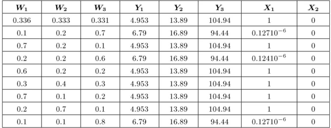
The sensitivity analysis on W1, W2and W3is shown in
Table 7.
By increasing Wi, the value of Yi would be
decreased. LINGO software was used to solve the above four problems. The corresponding comparisons are shown in Table 8. The above results were provided
Table 6. The range of objective functions.
Z1 Z2 Z3 X1 X2
max(Z1) -4.953 -13.89 -104.94 1 0
max(Z2) -5.0065 -13.876 -105.261 1 0.1071
max(Z3) -6.79 -16.89 -94.44 0 0
Table 7. The range of objective functions for dierent values of W1, W2 and W3.
W1 W2 W3 Y1 Y2 Y3 X1 X2
0.336 0.333 0.331 4.953 13.89 104.94 1 0
0.1 0.2 0.7 6.79 16.89 94.44 0.12710 6 0
0.7 0.2 0.1 4.953 13.89 104.94 1 0
0.2 0.2 0.6 6.79 16.89 94.44 0.12410 6 0
0.6 0.2 0.2 4.953 13.89 104.94 1 0
0.3 0.4 0.3 4.953 13.89 104.94 1 0
0.7 0.1 0.2 4.953 13.89 104.94 1 0
0.2 0.7 0.1 4.953 13.89 104.94 1 0
0.1 0.1 0.8 6.79 16.89 94.44 0.12710 6 0
Table 8. Optimal results of the existing methods and the proposed method.
X1 X2 Y1 Y2 Y3
Limited Goals Method 0.19 0.19 6.56 16.33 94.1
Derringer and Suich [13] 0.84 -1 4.77 15.87 100.26
Noorossana [17] 0.815 -1 4.81 15.96 100
Pasandideh and Niaki [1] 0.835 -0.99 4.78 15.86 100.23
Presented Method for
W1 = 0:7, W2= 0:2, W3= 0:1 1 0 4.953 13.89 104.94
Presented Method for
W1 = 0:1, W2= 0:2, W3= 0:7 0.12710
by assuming that W1 = 0:7, W2 = 0:2 and W3 = 0:1,
or W1 = 0:1, W2 = 0:2 and W3 = 0:7. The above
example was presented to evaluate the performance of the developed method.
CONCLUSION
The proposed method in this paper used fuzzy goal programming to determine the optimal solution of statistical multi-response problems. The proposed method solved (m + 1) problems to reach the optimal, m, responses. Two examples were presented to evalu-ate the performance of the developed method.
NOMENCLATURE
Uj upper bound of objective function Zj
Lj lower bound of objective function Zj
j access level to the optimum of objective
function Zj
Wj the importance or weight of objective
function Zj from the viewpoint of the
decision maker
(Zj) the fuzzy membership function of
objective function Zj
Z
j the optimal value of objective function
Zj
X
j the optimal value of variable Xj
j the tolerance of objective function Zj,
j= Uj Lj
REFERENCES
1. Pasandideh, S.H.R. and Niaki, S.T.A. \Multi-response simulation optimization using genetic algorithm within desirability function framework", Applied Mathematics and Computation, 175(1), pp 336-382 (April, 2006). 2. Suhr, R. and Baston, R.G. \Constrained multivariate
loss function minimization", Quality Engineering, pp 475-483 (2001).
3. Myers, R. and Carter, W.J. \Response surface tech-niques for dual response systems", Technometrics, pp 301-317 (1973).
4. Biles, W. \A response surface method for experimental optimization of multi response processes", Industrial and Engineering Chemistry, pp 152-158 (1973). 5. Myers, R., Khuri, A. and Vining, G. \Response surface
alternatives to the Taguchi robust parameter design approach", The American Statistician, pp 131-139 (1973).
6. Lo, Y. and Tang, K. \Economic design of multi charac-teristic models for a three class screening", Procedure Journal Product, pp 2341-2351 (1990).
7. Pignatiello, J.J. \Strategies for robust multi response", Quality Engineering, pp 5-15 (1993).
8. Winston, W.L., Operations Research Applications and Algorithms, 3rd Ed., Duxbury Press, Belmont, CA, USA (1994).
9. Artiles-Leon, N. \A pragmatic approach to multiple-response problems using loss functions", Quality Engi-neering, pp 213-220 (1996).
10. Ross, P.J., Techniques for Quality Engineering, 2nd Ed., McGraw-Hill, New York (1996).
11. Kapur, C.K. and Cho, B.R. \Economic design of the specication region for multiple quality characteris-tics", IIE Trans., pp 237-248 (1996).
12. Robert, G.B. and Richard, S. \Constrained multivari-ate loss function minimization", Quality Engineering, pp 475-483 (2001).
13. Derringer, G. and Suich, R. \Simultaneous optimiza-tion of several response variables", Journal of Quality Technology, 12, pp 214-219 (1980).
14. Zimmermann, H.J. \Fuzzy programming and linear programming with several objective functions", Fuzzy Sets and Systems, pp 45-55 (1978).
15. Cheng, C.B., Cheng, C.J. and Lee, E.S. \Neuro-fuzzy and genetic algorithm in multiple response optimiza-tion", Computers and Mathematics with Applications, 44, pp 1503-1514 (2002).
16. Keeney, R.L. and Raia H., Decisions with Multiple Objectives: Preferences and Value Tradeos, John Wiley, New York (1976).
17. Noorossena, R., Sultan Penah, H. \Oering a method for extracting D.M. function and using it for the multi-purpose optimization within the framework of RSM", International Journal of Engineering Science, 15, pp 221-233, University of Industry and Science, Iran (2003).