Two meta-heuristic algorithms for the dual-resource constrained flexible job-shop scheduling problem

Scientia Iranica

Transactions E: Industrial Engineering www.scientiairanica.com

Two meta-heuristic algorithms for the dual-resource

constrained exible job-shop scheduling problem

M. Yazdani

_{, M. Zandieh}

_{, R. Tavakkoli-Moghaddam}

_{and F. Jolai}

b. Department of Industrial Management, Faculty of Management and Accounting, Shahid Beheshti University, G.C., Tehran, Iran. c. School of Industrial Engineering, College of Engineering, University of Tehran, Tehran, Iran.

Received 27 November 2013; received in revised form 2 June 2014; accepted 21 June 2014

KEYWORDS Flexible job-shop scheduling; Dual-resource constrained;

Simulated annealing; Vibration damping optimization; Taguchi experimental design.

Abstract. Systems where both machines and workers are treated as constraints are termed Dual-Resource Constrained (DRC) systems. In the last few decades, DRC scheduling has attracted much attention from researchers. This paper addresses the Dual-Resource Constrained Flexible Job-Shop Scheduling Problem (DRCFJSP) to minimize makespan. This problem is NP-hard and mainly includes three sub-problems: (1) assigning each operation to a machine out of a set of compatible machines, (2) determining a worker among a set of skilled workers for operating each operation on the selected machine, and (3) sequencing the operations on the machines considering workers in order to optimize the performance measure. This paper presents two meta-heuristic algorithms, namely Simulated Annealing (SA), and Vibration Damping Optimization (VDO), to solve the DRCFJSP. The proposed algorithms make use of various neighborhood structures to search in the solution space. The Taguchi experimental design method as an optimization technique is employed to tune dierent parameters and operators of the presented algorithms. Numerical experiments with randomly generated test problems are used to evaluate performance of the developed algorithms. A lower bound is used to obtain the minimum value of makespan for the test problems. The computational study conrms the proper quality of the results of the proposed algorithms.

c

2015 Sharif University of Technology. All rights reserved.

1. Introduction

The Flexible Job-shop Scheduling Problem (FJSP) is an extension of the Job-shop Scheduling Problem (JSP), which provides a closer approximation to a wide range of scheduling problems encountered in real manufacturing systems [1]. FJSP mainly consists of two sub-problems, including assigning each operation to a machine out of a set of capable machines, and sequencing the assigned operations on the machines. In FJSP, in addition to sequencing of the operations

*. Corresponding author. Mobile: +98 9113310090; Fax: 02833675784

E-mail address: mehdi [email protected]

on the machines (diculty of JSP), assignment of the operations to the machines is also needed. Thus, The FJSP is more complex than the JSP. Mati and Xie [2] proved that the FJSP with two machines and one objective is also NP-hard.

Real world manufacturing systems are usually constrained by both machine and human resources. Human operators are often the constraining resource and transfer between workstations to process jobs when required. This type of system, in which both machines and workers represent potential capacity constraints on the shop capacity, is referred to as a Dual-Resource Constrained (DRC) shop [3]. The rst study on DRC research has been conducted by Nelson [4]. The FJSP considering worker and machine constraints, i.e.

Dual-Resource Constrained Flexible Job-shop Scheduling Problem (DRCFJSP), is one of the NP-hard problems in DRC environment.

It mainly consists of three sub-problems:

1. Assigning operations to resources of machines,

2. Assigning operations to resources of workers,

3. Sequencing the operations on the machines consid-ering workers in order to optimize the performance measure.

In this paper, the DRCFJSP with heterogeneous work-ers is considered as a main subject of research.

Most of DRC scheduling studies are performed in a job-shop environment. Some of researches in relation to the DRC Job-shop Scheduling Problem (DRCJSP) are as follows. Jaber and Neumann [5] propounded a mathematical model that described fatigue and re-covery in a DRCJSP with one worker performing n tasks within m cycles. Jingyao et al. [6] presented a hybrid algorithm based on ant colony optimization to solve the DRCJSP with heterogeneous workers (ACO). The algorithm established a dynamic candidate so-lution set, based on the technology constraint, for each ant to improve the calculating eciency of the algorithm. Jingyao et al. [7] presented a scheduling approach based on ACO for this problem. This hybrid algorithm utilized the combination of ACO and Simulated Annealing (SA) algorithm and employed an adaptive control mechanism based on ant ow of route choice to improve the global search ability. Jingyao et al. [8] proposed an inherited Genetic Algorithm (GA) to solve the double-objective optimization of the DRCJSP. In this algorithm, evolutionary experience of a parent population was inherited by the means of branch population supplement based on pheromones to accelerate the convergence rate. Lobo et al. [9] proposed a lower bound for the DRCJSP in which the objective is to minimize the maximum job lateness. This work is studied to eectively evaluate the absolute performance of heuristic solutions.

Few papers discussed DRC scheduling in a exible job-shop environment. Xianzhou and Zhenhe [10] proposed a new immune GA for the DRCFJSP through combining immune algorithm with the GA. Liu et al. [11] propounded a hybrid Pareto-based GA and applied it to the bi-objective DRCFJSP in which the makespan and the production cost were concerned. Lang and Li [12] presented an algorithm that combines grey simulation technology and Non-dominated Sort-ing Genetic Algorithm II (NSGA-II). They employed this algorithm for solving a multi-objective DRCFJSP under uncertainty. Lie and Guo [13] propounded a Variable Neighborhood Search (VNS) algorithm for solving the DRCFJSP. In this study, four neighborhood structures were applied to produce new solutions of

the DRCFJSP. Two neighborhood structures (i.e., Swap and Insert) were about operation sequence sub-problem. Two novel neighborhood structures (i.e., Assign and Change) were applied to another sub-problem of the DRCFJSP.

The diculty of the DRCFJSP suggests the adoption of mata-heuristic methods producing reason-ably good schedules in a reasonable time, instead of looking for an exact solution. SA algorithm is one of the well-known meta-heuristics which have been applied successfully to optimize various combinatorial optimization problems. Also, the Vibration Damp-ing Optimization (VDO) algorithm is a novel meta-heuristic algorithm that can be eciently used to solve such problems. In this paper, the authors develop SA and VDO algorithms for solving the DRCFJSP. These algorithms make the use of four neighborhood structures to search in the solution space. There exist lots of mathematical model formulated for FJSP with kinds of objectives [14-16]. But there is no comprehensive research about mathematical model of DRCFJSP. In this research, we propose a Mixed-Integer Linear Programming (MILP) model for the DRCFJSP based on precedence variables.

The rest of the paper is organized as follows. Section 2 presents denition of the problem. Section 3 presents a mathematical model for the DRCFJSP. The proposed algorithms for solving the DRCFJSP are introduced in Section 4. In Section 5, Taguchi experimental design is presented to tune the presented algorithms. The computational study performed with the proposed algorithms is informed in Section 6. The conclusion and some further research suggestions are presented in Section 7.

2. Problem denition

In DRCFJSP, the execution of n jobs on m machines by h workers is scheduled. In this problem, there are a set of jobs J = fJ1; J2; ; Jng, a set of machines

M = fM1; M2; ; Mmg and set of workers W =

fW1; W2; ; Whg. In fact, the process of jobs is

limited by the two resources, namely machines and workers. Each job Ji is formed by a sequence of

ni operations (Oi;1; Oi;2; ; Oi;ni) to be performed

one after the other based on the given order. Each operation Oi;j (i.e., the operation j of job i) can

be processed on any among a subset of capable ma-chines. Mi;j =

h

S

l=1Mi;j;l (for i = 1; 2; ; n and

j = 1; 2; ; ni) is the set of all compatible machines

that can be used to perform operation Oi;j in which

Mi;j;l is a set including machines eligible to process

Oi;j by worker l. Wi;j = m

S

k=1Wi;j;k (for i = 1; 2; ; n

including eligible workers to operate Oi;j on machine

k. The following are the assumptions made in solving this problem:

All machines and workers are available at time 0.

All jobs can be processed at time 0.

At a given time, a machine can execute at most one operation.

At a given time, a worker can operate at most one operation.

Each operation can be processed with dierent machine and dierent worker, while the practice processing time is dierent.

Processing times are deterministic and known in advance.

Each processing operation requires both the worker and machine.

Workers may be transferred from one machine to another.

Worker cannot be transferred during its processing.

Once an operation is started on a machine it must be completed before another operation can start on that machine (i.e., preemption of jobs is not allowed).

A worker can operate more than one machine, and one machine can be operated by dierent workers.

Setup time and unloading time are included in the processing time.

Transportation time between facilities is negligible or included in the processing time.

The purpose of the DRCFJSP is to assign each operation to a proper machine out of a set of capable machines, determine a worker among a set of skilled workers for processing operation on selected machine, and sequence the operations on the machines consider-ing workers such that the maximum completion time of all jobs (i.e., makespan) is minimized. Flexibility of the DRCFJSP is specied based on exibility of workers and machines. This exibility can be categorized into partial exibility and total exibility. It is total when we have Mi;j = M and Wi;j = W for all operations;

otherwise, it is partial. Data related to a given problem with four jobs, three machines, two workers and partial exibility is shown in Table 1. In this table, symbol 1 means that the operation cannot be processed on the corresponding machine and worker.

3. Mathematical model

In this section, a MILP model is presented for the DRCFJSP. We introduce some notations and proceed

Operations M1 M2 M3

W1 W2 W1 W2 W1 W2

O1;1 12 1 8 1 10 1

O1;2 16 13 10 11 10 15

O1;3 1 7 9 8 1 1

O2;1 6 7 9 10 1 7

O2;2 11 17 1 1 14 13

O3;1 1 1 4 9 1 8

O3;2 7 8 5 8 6 8

O3;3 1 18 1 16 1 15

O4;1 6 1 9 11 1 5

O4;2 1 15 17 13 1 1

by representing the MILP formulation. The related notations are rst listed below.

Parameters:

n Number of jobs m Number of machines h Number of workers

ni Number of operations of job i

Mi;j The set including machines eligible to

process Oi;j

Wi;j The set including workers eligible to

operate Oi;j

Mi;j;l The set including machines eligible to

process Oi;j by worker l

Wi;j;k The set including workers eligible to

operate Oi;j on machine k

pi;j;k;l Processing time of operation j of job i

on machine k by worker l Indices:

i; r Indices for jobs where f1; 2; ; ng j; s Indices for operations of job

k Index for machines where f1; 2; ; mg l Index for workers where f1; 2; ; hg Decision variables:

Xi;j;r;s Binary variable taking value 1 if Oi;j is

processed after Or;s; and 0, otherwise

Yi;j;k;l Binary variable taking value 1 if Oi;j

is processed on machine k by worker l; and 0, otherwise

Ci;j Continuous variable for the completion

time of Oi;j

Cmax Makespan

Under these notations, the considered DRCFJSP can be formulated as the following MILP model:

min Cmax,

s.t. X

k2Mi;j

X

l2Wi;j;k

Yi;j;k;l = 1 8i; j; (1)

Ci;j Ci;j 1+

X

k2Mi;j

X

l2Wi;j;k

Yi;j;k;l:pi;j;k;l 8i; j; (2)

Ci;j Cr;s+

X

l2Wi;j;k

Yi;j;k;l:pi;j;k;l M:(1 xi;j;r;s)

M: 0

@2 X

l2Wi;j;k

Yi;j;k;l

X

l2Wr;s;k

Yr;s;k;l

1 A

8i < n; j; r > i; s; k 2 fMi;j\ Mr;sg; (3)

Cr;s Ci;j+

X

l2Wi;j;k

Yr;s;k;l:pr;s;k;l M:xi;j;r;s

M: 0

@2 X

l2Wi;j;k

Yi;j;k;l

X

l2Wr;s;k

Yr;s;k;l

1 A

8i < n; j; r > i; s; k 2 fMi;j\ Mr;sg; (4)

Ci;j Cr;s+

X

k2Mi;j;l

Yi;j;k;l:pi;j;k;l M:(1 xi;j;r;s)

M: 0

@2 X

k2Mi;j;l

Yi;j;k;l

X

k2Mr;s;l

Yr;s;k;l

1 A

8i < n; j; r > i; s; l 2 fWi;j\ Wr;sg; (5)

Cr;s Ci;j+

X

k2Mi;j;l

Yr;s;k;l:pr;s;k;l M:xi;j;r;s

M: 0

@2 X

k2Mi;j;l

Yi;j;k;l

X

k2Mr;s;l

Yr;s;k;l

1 A

8i < n; j; r > i; s; l 2 fWi;j\ Wr;sg; (6)

Cmax Ci;ni 8i; (7)

Ci;j 0 8i; j; (8)

Xi;j;r;s; Yi;j;k;l2 f0; 1g 8 i; j; r; s; k; l; (9)

where Ci;0= 0.

Constraint (1) determines the machine and worker for processing each operation. Constraint (2) guarantees precedence constraints between the oper-ations of the same job. This constraint determines

completion time of an operation of a job in relation to previous operation of the same job (dierence between the completion times of operation Oi;jand its previous

operation of the same job must be at least equal to pi;j;k;l). Constraints (3) and (4) determine the

rela-tionship between completion times of two operations of dierent two jobs if these operations are implemented on the same machine. These two constraints handling one machine can only execute one operation at a given time. Constraints (5) and (6) determine relationship between completion times of two operations of dierent two jobs if these operations are executed by the same worker. These two constraints controlling one worker can only execute one operation at a given time. Constraint (7) calculates the makespan. Constraints (8) and (9) dene decision variables.

4. Proposed algorithms

In this section, we describe the proposed SA and VDO algorithms for solving the DRCFJSP. Section 4 is subdivided into the following 4 subdivisions.

Section 4.1 explains solution representation solu-tion method; neighborhood structures employed in the presented algorithms are claried in Section 4.2. In Section 4.3, the steps of the SA algorithm are reported. Next, the steps of the VDO algorithm are explained in Section 4.4.

4.1. Representation solution method

One important decision in designing a meta-heuristic method is to decide how to represent and relate solutions in an ecient way to the searching space [17]. In this article, the task sequencing list, proposed by Lei and Guo [13], is used to represent the DRCFJSP solution wherein a main string is made by subsidiary quadruple strings (i; j; k; l); one for each operation. In a quadruple string, i signies the job which an operation belongs to; j characterizes the progressive number of that operation within job i; k indicates the machine assigned to that operation; l indicates the worker assigned to that operation. The left-to-right ordering of operations in the solution string represents the sequencing of the operations on the machines. Consider the problem in the Table 1. The solution:

S = [(O4;1; M3; W2); (O1;1; M2; W1); (O4;2; M1; W2);

(O1;2; M3; W1); (O3;1; M2; W1); (O3;2; M2; W1);

(O1;3; M1; W2); (O2;1; M1; W1); (O3;3; M3; W2);

(O2;2; M1; W1)];

is an optimal solution from solution space for the mentioned problem shown in Table 1. The exhibition of this solution in the task sequencing list pattern is

Figure 1. Representation of solution S.

Figure 2. Gantt chart for machines and workers.

presented in Figure 1. Furthermore, Figure 2 shows the Gantt chart of this solution for both machines and workers separately where makespan equals 44.

4.2. Neighborhood structures

The technique of moving from one solution to its neighboring solution is delineated by a key factor known as neighborhood structure [18]. In the proposed algorithms, four types of neighborhood structures are used. The rst one improves the operation-machine assignment, while the second one is to improve the operation-worker assignment. The third and fourth are to improve the operation sequence. The third one changes the positions of two operations while the fourth one makes larger alter by changing the positions of operations of two jobs.

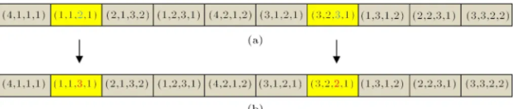
4.2.1. Assignment Neighborhood Structure-1 (ANS-1) The rst neighborhood structure is called ANS-1. In this neighborhood structure, d randomly selected op-erations are randomly reassigned to another machine, among the eligible machines of that operation. Since only eligible machines are considered for each

oper-ation, the new generated solution is always feasible. If the problem size is small, we have d = 1. For medium and large problem size, we have d = 2 and 3, respectively. Note that the assignment of the operations to the workers and sequencing of the operations on the machines remains unchanged.

To further illustrate the procedure, consider a problem with four jobs, three machines, two workers and ten operations. One possible solution is shown by Figure 3(a). Suppose we have d = 2, and then, the two randomly selected operations are O1;1 and

O3;2. In the current solution, O1;1has been assigned to

Machine 2 and O3;2 to Machine 3. By reassigning these

two operations to dierent eligible machines, a new solution is obtained. Again suppose O1;1 is reassigned

to Machine 3 and O3;2 is also reassigned to Machine 2.

Figure 3(b) shows the new generated solution. 4.2.2. Assignment Neighborhood Structure-2 (ANS-2) This neighborhood structure is called ANS-2. Like ANS-1, d operations are randomly selected. But, each one is reassigned to another worker, among eligible workers of that operation. In this case, the new generated solution is also feasible. Again value of d depends on the problem size. If the problem is small, then we have d = 1. For medium and large problem sizes, we consider d = 2 and 3, respectively. Note that ANS-2 does not change any of operation-machine assignment and sequence of operations.

Consider the abovementioned example. Fig-ure 4(a) displays one possible solution to this problem. Suppose we have d = 2 and the two randomly selected operations are O4;2 and O3;3. In the current solution,

both operations O4;2 and O3;3 have been assigned to

worker 2. To generate a new solution, these two operations are reassigned to worker 1. Figure 4(b) shows the new generated solution.

4.2.3. Sequence Neighborhood Structure-1 (SNS-1) The third neighborhood structure is named SNS-1. This structure focuses on sequence of operations. Both operation-machine and operation-worker assignments remain untouched. In this neighborhood structure, d times the following procedure is performed. The

Figure 4. The procedure of neighborhood structure ANS-2.

positions of two randomly selected adjacent operations are replaced. These replacements are performed con-sidering the priority constraints among the operations of the same job. If the problem size is small, we consider d = 2. For medium and large sizes, we have d = 4 and 6. Note that if the two randomly selected adjacent operations belong to two dierent jobs, the swap is carried out; otherwise (i.e., they belong to the same job), swap is avoided and two new adjacent operations are selected for swapping. To describe why swapping of the operations of the same job is avoided, let us remind the reader that each job has a xed processing route among its operations. That is, for job i, the processing route is fOi;1; Oi;2; ; Oi;nig where

ni is number of operations of job i. If the selected

adjacent operations belong to the same job and they are swapped, then the processing route of that job is violated. Hence, the new generated solution becomes infeasible.

To better describe SNS-1, we apply the procedure to the abovementioned example. Figure 5(a) shows one possible solution. Suppose d = 2, and the rst and second two randomly selected adjacent operations are (O1;2; O4;2) and (O1;3; O2;2). By swapping the

positions of these two pair of adjacent operations, the new generated solution, shown in Figure 5(b), is obtained.

4.2.4. Sequence Neighborhood Structure-2 (SNS-2) The fourth neighborhood structure is called SNS-2. In this neighborhood structure, two jobs are randomly selected. We have two cases:

Case 1. If the two jobs have the same number of operations, the following steps are performed:

Step 1: The operations of unselected jobs are copied into the same positions in new solution;

Step 2: The operations of the rst selected job are

copied into the positions of the second selected job with respect to sequencing constraints;

Step 3: The operations of the second selected job are copied into the positions of the rst selected job with respect to sequencing constraints. After implementing Step 3, the new solution is com-pleted.

Case 2. If the two jobs do not have the same number of operations, the following steps are done:

Step 1: The operations of unselected jobs are copied into the same positions in new solution;

Step 2: The operations of the job with lower number of operations, say e operations, are copied into the rst e positions of the other job (the job with greater number of operations) with respect to sequencing constraints;

Step 3: The operations which are related to the job with a greater number of operations are copied into the empty positions with regard to se-quencing constraints.

After Step 3 of this case, we also have a new com-plete solution. Note that the operation-machine and operation-worker assignments are not changed.

Consider an example with four jobs, three ma-chines and two workers and ten operations. One possible solution is shown by Figure 6. Suppose the randomly selected jobs are jobs 1 and 3. Since they have the same number of operations, the procedure of Case 1 is used. Figure 6 shows the steps of this procedure.

For the second case, consider the abovementioned example but suppose job 3 has 2 operations. Figure 7 shows one possible solution for this problem. Again, consider the selected jobs are jobs 1 and 3. Notice

Figure 6. Process of neighborhood structure SNS-2 in Case 1.

Figure 7. Process of neighborhood structure SNS-2 in Case 2.

that jobs 1 and 3 do not have the same number of operations. Therefore, the procedure of Case 2 is used. Figure 7 shows the steps of this procedure.

4.3. Simulated annealing

SA is a well-known meta-heuristic which have been ap-plied successfully to various combinatorial optimization problems [19,20]. This algorithm is capable of escaping from the local optima by permitting moves to inferior solutions during the search process. SA algorithm was rst proposed by Kirkpatrick et al. [19].

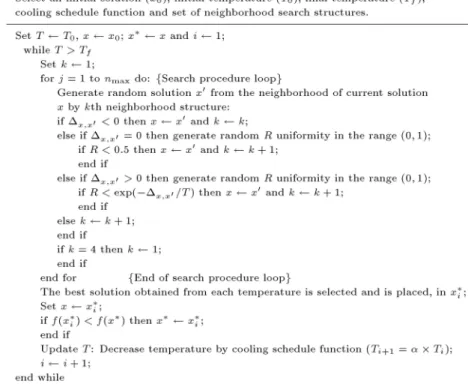
This subsection presents a SA algorithm for op-timizing the DRCFJSP. Figure 8 demonstrates the process of the proposed SA algorithm. At rst, initial solution, parameters of the algorithm and neighbor-hood structures are dened in the initialization step. In the next step, search procedure is performed with the input solution and set temperature. In this step, the neighboring solution x0 _{is generated from}

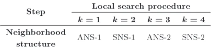
the neighborhood of current solution x by means of one neighborhood structure. In Figure 8, the order of employed neighborhood structures is indicated by parameter k. Table 2 species the type of implemented neighborhood structures in the search procedure. In continuation of the search process, the dierence be-tween x and x0₍

x;x0) is computed in terms of objective

Table 2. Neighborhood structures employed in the search procedure.

Step Local search procedure k = 1 k = 2 k = 3 k = 4 Neighborhood

structure ANS-1 SNS-1 ANS-2 SNS-2

function value. If x;x0 < 0, the current solution x

is replaced with neighboring solution x0_{(x x}0_{). In}

case of x;x0 = 0, a uniform random number (i.e.,

R U(0; 1) is generated. If R < 0:5, x is replaced with x0_{. Also, in case of}

x;x0 > 0, to decrease

the probability to get stuck in local optima, the SA may accept to move to an inferior neighboring solution depending on a randomized structure [21]. In this condition, x is replaced with x0_{, only if uniform random}

number R < exp( x;x0=T ) where R U(0; 1) and T

is current temperature. If none of the cases above is met, the current solution x is preferred.

After completion of the search procedure itera-tions in each temperature, the best solution of the search procedure, x

i, is chosen and it will be assigned

as the input solution of the search procedure in the subsequent temperature (x x

i). Besides, if xi

is better than the best solution having found in the searches so far (i.e., x_{), x is replaced with x}

i(x

x i).

Classically, the probability to accept bad moves (i.e., moves with increase in terms of objective function value) is high at the beginning to allow the algorithm to escape from local minimum. This probability decreases in a progressive way by reducing the temperature. The method used to decrease the temperature is generally called cooling schedule [22]. An applicable initial temperature should be high enough to generate equal chance for all states of the search space to be visited, and it should not be rather too high to perform quite a lot of redundant searches in high temperature [21]. At the end of iterations of the search procedure of SA algorithm (after the number of search procedure iterations at one temperature level is nished), the

Figure 8. Steps of the proposed SA for the DRCFJSP.

current temperature will be decreased by the cooling schedule function. In this paper, we apply the following function to decrease the temperature:

Ti+1= Ti; (10)

where is a constant cooling rate. The cooling rate is dened as less than and close to 1.0. Typically the cooling rate is specied as between 0.8 and 0.99 [23].

The presented SA algorithm continues until the stopping criterion (i.e., nal temperature) is achieved. When the process of the algorithm stops, the nal solution x _{is used as the best solution. The nal}

temperature (Tf) is set to be 0.01. Initial temperature

(T0), number of neighborhood searches in the search

procedure for each temperature (nmax) and cooling rate

() are determined in the parameter tuning section. 4.4. Vibration damping optimization

In physics, vibration is dened as the oscilla-tion/repetitive motion of an object around an equi-librium position [24] where the object position is obtained when no force acts on it. The vibration of an object comes from an excitation force, may either be externally applied to the object or originate inside the object. In vibration phenomenon, the reduction process of amplitude of oscillation, tending to zero over time, is called vibration damping process. There is a useful connection between the vibration damping process and optimization. In the analogy between an optimization problem and the vibration damping process:

I) The states of oscillation system represent feasible solutions of the optimization problem;

II) The energies of the states correspond to the objec-tive function value computed at those solutions;

III) The minimum energy state corresponds to the optimal solution and rapid quenching can be viewed as local optimization.

In the solving methodologies area, Mehdizadeh and Tavakkoli-Moghaddam [25] introduced a new meta-heuristic algorithm, namely Vibration Damping Op-timization (VDO). This stochastic search method is inspired by the SA algorithm and is created based on the concept of the vibration damping in mechanical vibration [26,27].

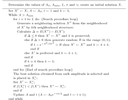
In this subsection, the VDO algorithm is pre-sented for solving the DRCFJSP. Figure 9 shows the process of the proposed VDO algorithm. During the initialization step of the proposed algorithm, initial amplitude (A0), minimum amplitude (Amin), number

of neighborhood searches in the search procedure for each amplitude (L), damping coecient () and sigma of Rayleigh distribution () are determined. The amplitude in the suggested algorithm has a control parameter role. This factor controls the possibility of the acceptance of a worse solution in various steps of the algorithm. At high amplitude (early in the search), there is some exibility to move to a worse solution; however, at lower amplitude (later in the search) less of this exibility exists. The algorithm escapement from local optimum is reduced in low

Figure 9. Steps of the proposed VDO for the DRCFJSP.

amplitude and the accessibility to global optimization is increased in higher amplitude. In addition, in the initialization step, an initial solution X is generated randomly and is set as the current solution X0_(X0

X). In the next step of the VDO algorithm, search procedure is performed. In each iteration of the search procedure, a new neighboring solution X00 _is

generated by implementing a neighborhood structure on the current solution X0_{. It is noted that type and}

order of neighborhood structures of the proposed VDO algorithm are equivalent to the proposed SA algorithm. After the neighboring solution X00 _{is produced, the}

dierence in objective function value ( = E(X00₎

E(X0_{)) is computed. If the dierence is negative or}

zero (i.e., 0), current solution X0 _{is replaced}

with neighboring solution X00_(X0 _X00_{). Besides, In}

the case of positive dierence ( > 0), the algorithm moves from current solution X0_{to neighboring solution}

X00_{, only if 1 e} A2₌₂2

> R where R U(0; 1), A is current amplitude and is sigma of a Rayleigh distribution. This leaves the possibility of nding a global optimal solution out of a local optimum [28]. If none of the conditions above is met, the current solution X0 _{is preferred. On a condition that all}

iterations of the search procedure are considered, one iteration of the VDO algorithm is accomplished. In that case, the stopping condition is checked. If this condition is not met, the next iteration of the algorithm begins with new amplitude (A A0e t=2).

Otherwise, the algorithm is terminated. There are many rules for the stopping condition in meta-heuristic algorithms, which depends on the problem at hand. Some of them for the VDO algorithm can be as follows:

1. Maximum number of iterations;

2. Reaching to the point that iteration will not im-prove quality solution afterwards;

3. Reaching to minimum amplitude Amin.

In this paper, the VDO algorithm continues until pre-specied minimum amplitude (Amin) is achieved.

Amin is set to be 10 6. Values of A0, , L and are

determined in the parameter tuning section.

5. Parameter tuning

For parameter calibration of algorithms, several meth-ods to statistically design the experiment are available. Among all, the Taguchi experimental design method [29,30] has shown great success for the parameter design stage to nd optimal process settings in dierent elds [31-33]. In this method, the orthogonal arrays are used to study a large number of decision variables with a small number of experiments. The Taguchi method separates the factors into two main groups: controllable and noise factors. Controllable factors will be placed in the inner orthogonal array and noise factors in the outer orthogonal array. Due to unpractical and often impossible omission of the noise factors, the Taguchi method tends to both minimize the impact of noise and also nd the best level of the inuential controllable factors on the basis of robustness.

The Taguchi method has created a transformation of the repetition data to another value that is the measure of variation. The transformation is the Signal-to-Noise (S/N) ratio that explains why this type of the parameter design is called robust design [30]. Here, the term \signal" denotes the desirable value (i.e., mean

response variable) and \noise" denotes the undesirable value (i.e., standard deviation) [31]. So the S/N ratio indicates the amount of variation present in the response variable. In the Taguchi method, the S/N ratio of the minimization objectives is given below [32]:

S/N ratio : 10 log₁₀ 1 n

n

X

i=1

y2 i

!

[db]; (11)

where y is the response variable and n is the number of experiments. It should be noted that the S/N ratios are exposed in terms of the desi-bell (db) scale. The aim is to maximize the S/N ratio [34].

In this paper, we apply the Taguchi method in parameter setting to achieve better robustness of the SA and VDO algorithms. Control factors of SA algorithm are: Initial temperature (T0), number of

neighborhood searches in the search procedure for each temperature (nmax) and cooling rate (). Also, VDO

control factors are: Initial amplitude (A0), sigma of

Rayleigh distribution (), number of neighborhood searches in the search procedure for each amplitude (L) and damping coecient (). Levels of these factors are illustrated in Tables 3 and 4.

To select the appropriate orthogonal array for tuning the SA, it is necessary to calculate the total degree of freedom. The proper array should contain a degree of freedom for the makespan and three degrees of freedom for each factor with four levels (3 3 = 9). Thus, the sum of the required degrees of freedom is 1 + 3 3 = 10. Therefore, the appropriate array should have at least 10 rows. From the standard table of orthogonal arrays, L16is selected as the ttest

orthogonal array design that fullls our all minimum requirements. The modied orthogonal array L16 is

presented in Table 5 in which control factors are assigned to the columns of the orthogonal array and

Table 3. Factors and their levels for the SA algorithm.

Factors Symbols Levels

Initial temperature (T0) A

A(1)-10 A(2)-20 A(3)-30 A(4)-40 Number of neighborhood

searches in the search procedure for each temperature (nmax)

B

B(1)-100 B(2)-150 B(3)-200 B(4)-250

Cooling rate () C

C(1)-0.8 C(2)-0.85

C(3)-0.9 C(4)-0.95

the corresponding integers in these columns indicate the actual levels of these factors.

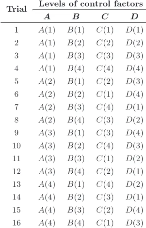
Also, to determine the proper orthogonal array for setting the VDO, we calculate the total degree of freedom. The appropriate array should comprise a degree of freedom for the makespan and three degrees of freedom for each factor with four levels (4 3 = 12). Thus, the sum of the required degrees of freedom is

Table 4. Factors and their levels for the VDO algorithm.

Factors Symbols Levels

Initial amplitude (A0) A

A(1)-5 A(2)-10 A(3)-15 A(4)-20 Sigma of Rayleigh

distribution () B

B(1)-0.5 B(2)-1 B(3)-1.5

B(4)-2 Number of neighborhood

searches in the search procedure for each amplitude (L)

C

C(1)-100 C(2)-150 C(3)-200 C(4)-250

Damping coecient () D

D(1)-0.05 D(2)-0.1 D(3)-0.15

D(4)-0.2 Table 5. The modied orthogonal array L16for tuning the SA algorithm.

Trial Levels of control factors

A B C

1 A(1) B(1) C(1)

2 A(1) B(2) C(2)

3 A(1) B(3) C(3)

4 A(1) B(4) C(4)

5 A(2) B(1) C(2)

6 A(2) B(2) C(1)

7 A(2) B(3) C(4)

8 A(2) B(4) C(3)

9 A(3) B(1) C(3)

10 A(3) B(2) C(4) 11 A(3) B(3) C(1)

12 A3) B(4) C(2)

13 A(4) B(1) C(4) 14 A(4) B(2) C(3) 15 A(4) B(3) C(2) 16 A(4) B(4) C(1)

the VDO algorithm.

Trial Levels of control factors

A B C D

1 A(1) B(1) C(1) D(1) 2 A(1) B(2) C(2) D(2) 3 A(1) B(3) C(3) D(3) 4 A(1) B(4) C(4) D(4) 5 A(2) B(1) C(2) D(3) 6 A(2) B(2) C(1) D(4) 7 A(2) B(3) C(4) D(1) 8 A(2) B(4) C(3) D(2) 9 A(3) B(1) C(3) D(4) 10 A(3) B(2) C(4) D(3) 11 A(3) B(3) C(1) D(2) 12 A(3) B(4) C(2) D(1) 13 A(4) B(1) C(4) D(2) 14 A(4) B(2) C(3) D(1) 15 A(4) B(3) C(2) D(4) 16 A(4) B(4) C(1) D(3)

1 + 4 3 = 13. Therefore, the appropriate array should have at least 13 rows. From the standard table of orthogonal arrays, L16 is selected as the ttest

orthogonal array design that fullls our all minimum requirements. The modied orthogonal array L16 is

presented in Table 6.

For parameter tuning, 10 test problems with dierent sizes and specications are generated. To yield more reliable information and because of having a stochastic nature of the presented algorithms, we tackle each test problem ve times. Therefore, we have 50 results for each trial to set parameters. In parameter tuning step, the stop conditions is the same for SA and VDO algorithms and equal to allowed computational times. After obtaining the results of the test problems in dierent trials, the results of each trial are transformed into the S/N ratio. The S/N ratios of trials are averaged in each level, and its value is plotted against each control factor. The average S/N ratio plot for SA and VDO algorithms are shown in Figures 10 and 11, respectively. As indicated

Figure 10. The average S/N ratio plot at each level of the factors for objective function values in SA.

is achieved when the parameters are set as follows: T0: A(2) = 20, nmax: B(3) = 200 and : C(3) = 0:9.

Also, based on information of Figure 11 the best chosen levels for VDO are as follows: A0: A(1) = 5, :

B(3) = 1:5, L: C(3) = 150 and : D(4) = 0:2.

6. Computational results

The proposed MILP model and algorithms are evalu-ated in this section. In the following subsections, at rst the MILP model is assessed, and then algorithms are evaluated. To conduct the experiments, we use a PC with 3.2 GHz (Core I7) and 8 GB of RAM memory for performing computational study. Minimization of the makespan is considered as the objective function. 6.1. MILP model's evaluation

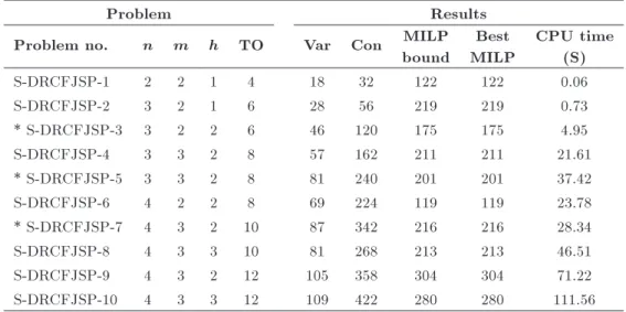
Here, the validity of the proposed MILP model is eval-uated in terms of size and computational complexities. In the size complexity evaluation, models are exam-ined on the basis of the numbers of binary variables, continuous variables and constraints generated by the nature of the models. Table 7 shows the number of binary variables, continuous variables and constraints related to the proposed mathematical model with n jobs, m machines and h workers where each job has m operations.

Next, using CPLEX 12 software, we assess com-putational complexity of the proposed model (i.e. the models' capability to solve dierent problem sizes). We generate a DRCFJSP data set with 10 test problems in small sizes (S-DRCFJSP). The processing times of the problems are uniformly distributed over [1, 99]. These test problems are formulated by the MILP model described in Section 3 \mathematical model", and then the models are solved by CPLEX software. Charac-terizes of the generated test problems and obtained results of the MILP model are shown in Table 8. Columns 1 to 5 represent characterizes of the problems in which n stands for the number of jobs, m embodies the number of given machines, h species the number of workers and TO represents the total number of operations for each problem. The number of variables and constraints related to the mathematical model, are respectively, shown in columns 6 and 7. Also, columns 8 to 10 signify the MILP bound (a bound on the best possible value of the objective can be attained

Table 7. Size complexity of the proposed mathematical model.

Factor Model

No. of binary variables nm2 _{h +}n 1 2

No. of continuous variables nm

Figure 11. The Average S/N ratio plot at each level of the factors for objective function values in VDO. Table 8. Obtained results of the MILP model by CPLEX software on small-sized problems.

Problem Results

Problem no. n m h TO Var Con MILP

bound

Best MILP

CPU time (S)

S-DRCFJSP-1 2 2 1 4 18 32 122 122 0.06

S-DRCFJSP-2 3 2 1 6 28 56 219 219 0.73

* S-DRCFJSP-3 3 2 2 6 46 120 175 175 4.95

S-DRCFJSP-4 3 3 2 8 57 162 211 211 21.61

* S-DRCFJSP-5 3 3 2 8 81 240 201 201 37.42

S-DRCFJSP-6 4 2 2 8 69 224 119 119 23.78

* S-DRCFJSP-7 4 3 2 10 87 342 216 216 28.34

S-DRCFJSP-8 4 3 3 10 81 268 213 213 46.51

S-DRCFJSP-9 4 3 2 12 105 358 304 304 71.22

S-DRCFJSP-10 4 3 3 12 109 422 280 280 111.56

in the given time), the best MILP (the objective value of the best integer solution found by the CPLEX within the given time limit) and computational time of the CPLEX software, respectively. The problems with total exibility are highlighted by symbol (*) in Table 8. The results in Table 8 indicate that the optimal solutions are obtained for test problems 1 to 10 (S-DRCFJSP) in a reasonable computational time. This outcome reveals the mathematical model can be applied for programming and optimizing the small-sized DRCFJSP problems. Note that we also used a mathematical model to solve larger problems. But due to complexity of the mathematical model in problems larger than problems in Table 8, CPLEX cannot obtain the optimal solution.

6.2. Algorithm's evaluation

This subsection describes the computational study which is used to evaluate the eectiveness and eciency of the proposed VDO and SA algorithms. In order to conduct the experiment, we implement the algorithms in MATLAB R2012b. The non-deterministic nature of the presented algorithms makes it necessary to carry

out multiple runs on the same problem instance in order to obtain reliable results. Therefore, the best solution is selected for each problem after ten runs of the given algorithm from dierent initial solutions.

The rst dataset under investigation is S-DRCFJSP. We perform VDO and SA algorithms on these problems. The result revealed that both algo-rithms have obtained optimal solutions in all 10 test problems. To perform extensive computational study, we generate a DRCFJSP data set with 20 test problems in medium and large sizes. Ten of these test problems are generated in medium sizes (M-DRCFJSP) and other ten test problems are generated in large sizes (L-DRCFJSP). The processing times of the problems are uniformly distributed over [1, 99]. Table 9 compares the results of the proposed SA and VDO algorithms on medium and large-sized problems. The rst column up to the fth one represents characterizes of the problems, in which n stands for the number of jobs, m embodies the number of given machines, h species the number of worker and TO represents the total number of operations for each problem. Problems with the total exibility are highlighted by symbol (*) in

Problem Results of SA Results of VDO

Problem no. n m h TO Lower

bound

Best SA

Average of solutions

Best VDO

Average of solutions

* M-DRCFJSP-1 5 3 2 15 435 447 447 447 447

M-DRCFJSP-2 6 3 2 18 496 507 509.5 507 507

M-DRCFJSP-3 6 4 2 25 537 550 553.4 547 547.8

* M-DRCFJSP-4 7 4 3 35 679 701 701 692 694.6

M-DRCFJSP-5 8 4 3 40 613 659 663.5 652 652

M-DRCFJSP-6 9 5 3 45 660 712 718.3 684 691.2

* M-DRCFJSP-7 10 5 3 50 773 820 821.8 805 810.7

M-DRCFJSP-8 10 6 3 60 946 1019 1031.1 984 993.3

* M-DRCFJSP-9 10 6 4 70 817 923 934.6 892 902.5

M-DRCFJSP-10 12 6 4 80 949 1091 1103.1 1045 1062.2

* L-DRCFJSP-1 15 6 4 90 1035 1166 1182.5 1109 1121.4

L-DRCFJSP-2 20 7 5 100 886 1059 1073.8 987 1002.1

L-DRCFJSP-3 20 8 5 120 1090 1241 1260.6 1168 1189.4

* L-DRCFJSP-4 20 8 6 120 954 1112 1128.2 1021 1035.3

L-DRCFJSP-5 30 10 7 150 984 1187 1227.4 1099 1123.8

* L-DRCFJSP-6 30 10 7 200 1292 1513 1549. 5 1396 1428.5

L-DRCFJSP-7 30 10 8 200 1188 1442 1486.2 1276 1307.5

* L-DRCFJSP-8 40 10 8 240 1309 1594 1618.1 1464 1485.2

L-DRCFJSP-9 50 10 8 300 1713 2139 2158.8 1986 2015.1

*L-DRCFJSP-10 50 10 8 300 1628 1980 2005.4 1817 1842.8

Table 9. In this paper, we make use of a lower bound of makespan proposed by Lei and Guo [13] for evaluating and comparing obtained results. This lower bound is attained in the following way: An earliest starting time of operation (rij) is rst calculated, ri1= qi(where qiis

the release time of the ith job), ri(j+1)= rij+~ij, ~ij=

min

k;l fpijklg, where i = f1; 2; ; ng, 1 j ni 1

and pijkl indicates the processing time of operation

Oi;j processed on machine k and operated by worker

l. Then, the values of the earliest starting time are ranked ascending. The sorted earliest starting time are imported in set R = fri1j1; ri2j2; ; r1NjNg, where N

is the total number of operations. The lower bound of the makespan is then obtained by:

Clow

max= max max_i

qi+

X

j

~ij

;

~

ERm+ P

i

P

j~ij

m

;

~

ERh+ P

i

P

j~ij

h

!

; (12)

where ~E is a numerical function dened as follows:

if x is integer, ~E(x) = x, else ~E(x) = x + 1; m indicates number of machines, w species the number of workers, Rm is the sum of the m (number of

machines) smallest values of the earliest start time from set R(Rm = Pml=1riljl) and Rh is the sum of the h

(number of workers) smallest values of the earliest start time from set RRh=Phl=1ril; jl

. In this paper, it is assumed that all jobs can be started at time 0(qi=

0). The values of the lower bound for the generated test problems are shown in the sixth column. The seventh column signies the best makespan obtained from ten runs of the SA algorithm, and the eighth column reports the average of the obtained results of ten runs. The ninth column shows the best makespan obtained from ten runs of the VDO, and the tenth column reports the average of the obtained results of ten runs. The results of Table 9 show that VDO works better than SA in medium- and large-sized problems.

For more investigations in the computational results and comparing the performances of these two algorithms, we use the Relative Percentage Deviation (RPD) measure computed by:

RPD = Algsol LB

LB 100%; (13) where Algsol is the objective function value obtained

Table 10. Results of RP D for the SA and VDO in medium-sized problems (M-DRCFJSP-1:10). Algorithm

SA VDO

Average RP D Standard

deviation RP D Average RP D

Standard deviation RP D

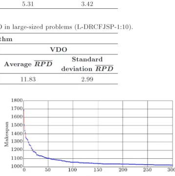
7.47 4.87 5.31 3.42

Table 11. Results of RP D for the SA and VDO in large-sized problems (L-DRCFJSP-1:10). Algorithm

SA VDO

Average RP D Standard

deviation RP D Average RP D

Standard deviation RP D

21.19 4.08 11.83 2.99

by the given algorithm and LB is the lower bound for objective function of the problem. Since 10 runs of algorithm are performed for each test problem, RPD should be calculated for result of each run. Then mean RPD results of runs (RP D) is computed and used for making comparisons among algorithms.

Tables 10 and 11 shows the average and standard deviation of RP D values related to the results of SA and VDO algorithms on medium and large-sized problems, respectively. As indicated in Table 10, the best performance in medium size is obtained by the VDO with the average RP D of 5.31% and the standard deviation RP D of 3.42%. Further-more, as can be seen in Table 11, the VDO achieves the best performance in large size with the average RP D of 11.83% and the standard deviation RP D of 2.99%. In order to verify the statistical validity of the results, we perform two-sample Student's t-test for medium- and large-sized problems, separately. The condence level is set to be 95% ( = 0:05). The tests have been accomplished using MINITAB 15.0 software. Based on t-test result for medium-sized problems, p-value becomes 0.267. Since p-value is higher than , there is not a clear statistically signicant dierence between performances of the VDO and SA algorithms in medium-sized problems and they provide statistically the same performance. Based on t-test result for large-sized problems, p-value becomes 0.00. Since p-value is lower than , there is a clear statistically signicant dierence between perfor-mances of the VDO and SA algorithms in large-sized problems. Therefore, the proposed VDO statistically works better than the proposed SA in large-sized problems.

The results obtained from VDO algorithm re-vealed the appropriate performance of our algorithm in optimizing large-sized problems. For instance, Figure 12 depicts the diagram of the algorithm conver-gence to minimize makespan for problem

L-DRCFJSP-Figure 12. Convergence of the VDO algorithm to minimize the makespan for problem L-DRCFJSP-4.

4. The best makespan which equals to 1021 is reached after 300 iterations.

7. Conclusions and future study

This paper has addressed the dual-resource constrained exible job-shop scheduling problem (DRCFJSP) to minimize the makespan. We presented a mixed integer linear programing model for DRCFSP. Additionally, we have developed two ecient meta-heuristic, namely SA and VDO, for solving the given problem. The search procedure of both algorithms used four ecient neighbourhood structures to search the solution space. In order to adjust the parameters and operators of the proposed algorithms, the Taguchi parameter design method has been used. To evaluate the proposed SA and VDO algorithms, we have performed the computational study with the generated dataset. The computational results have shown that the proposed VDO has worked better than the proposed SA statis-tically. In the following, some suggestions are oered for future studies:

Developing a hybrid meta-heuristic algorithm, such as VNS-SA and GA-VNS for solving DRCFJSP;

Considering sequence-dependent setup times as an important factor in the DRCFJSP;

heuristic algorithms for a multi-objective DRCFJSP considering other objective functions.

References

1. Amiri, M., Zandieh, M., Yazdani, M. and Bagheri, A. \Variable neighbourhood search algorithm for the exible job-shop scheduling problem", International Journal of Production Research, 48(19), pp. 5671-5689 (2010).

2. Mati, Y. and Xie, X. \The complexity of two-job shop problems with multi-purpose unrelated machines", Eu-ropean Journal of Operational Research, 152(1), pp. 159-169 (2004).

3. Sun, Z.J. and Zhu, J.Y. \Intelligent optimization for job shop scheduling of dual-resources", Journal of Southeast University (Natural Science Edition), 35(3), pp. 376-381 (2005).

4. Nelson, R.T. \Labor and machine limited production systems", Management Science, 13(9), pp. 648-671 (1967).

5. Jaber, M.Y. and Neumann, W.P. \Modelling worker fatigue and recovery in dual-resource constrained sys-tems", Computers & Industrial Engineering, 59(1), pp. 75-84 (2010).

6. Jingyao, L., Shudong, S., Yuan, H. and Ganggang, N. \A hybrid algorithm for scheduling of dual-resource constrained job shop", International Conference on Computing, Control and Industrial Engineering, pp. 235-238 (2010).

7. Jingyao, L., Shudong, S., Yuan, H. and Ganggang, N. \Research on double-objective optimal scheduling algorithm for dual resource constrained job shop", Articial Intelligence and Computational Intelligence; Lecture Notes in Computer Science, 6319, pp. 222-229 (2010).

8. Jingyao, L., Shudong, S. and Yuan, H. \Adaptive hy-brid ant colony optimization for solving dual resource constrained job shop scheduling problem", Journal of Software, 6(4), pp. 584-594 (2011).

9. Lobo, B.J., Hodgson, T.J., King, R.E., Thoney, K.A. and Wilson, J.R. \An eective lower bound max L in a worker-constrained job shop", Computers & Operations Research, 40(1), pp. 328-343 (2013).

10. Xianzhou, C. and Zhenhe, Y. \An improved genetic algorithm for dual-resource constrained exible job shop scheduling", Fourth International Conference on Intelligent Computation Technology and Automation (ICICTA), pp. 42-45 (2011).

11. Liu, X.X., Lio, C.H. and Tao, Z. \Research on bi-objective scheduling of dual-resource constrained exi-ble job shop", Advanced Materials Research, 211-212, pp. 1091-1095 (2011).

12. Lang, M.T. and Li, H. \Research on dual-resource

certainty", In Proceedings of 2nd International Con-ference on Articial Intelligence, Management Science and Electronic Commerce, pp. 1375-1378 (2011).

13. Lei, D. and Guo, X. \Variable neighbourhood search for dual-resource constrained exible job shop schedul-ing", International Journal of Production Research, 52(9), pp. 2519-2529 (2014).

14. Fattahi, P., Saidi Mehrabad, M. and Jolai, F. \Math-ematical modeling and heuristic approaches to exible job shop scheduling problems", Journal of Intelligent Manufacturing, 18(3), pp. 331-342 (2007).

15. Demir, Y. and Isleyen, S.K. \Evaluation of mathemat-ical models for exible job-shop scheduling problems", Applied Mathematical Modelling, 37(3), pp. 977-988 (2013).

16. Dousthaghi, S., Tavakkoli-Moghaddam, R. and Makui, A. \Solving the economic lot and delivery scheduling problem in a exible job shop with unrelated paral-lel machines and a shelf life by a proposed hybrid PSO", International Journal of Advanced Manufactur-ing Technology, 68(5-8), pp. 1401-1416 (2013).

17. Tavakkoli-Moghaddam, R., Azarkish, M. and Sadegh-nejad, A. \Solving a multi-objective job shop schedul-ing problem with sequence-dependent setup times by a Pareto archive PSO combined with genetic operators and VNS", International Journal of Advanced Manu-facturing Technology, 53(5-8), pp. 733-750 (2011).

18. Yazdani, M., Amiri, M. and Zandieh, M. \Flexible job-shop scheduling with parallel variable neighborhood search algorithm", Expert System with Applications, 37(1), pp. 678-687 (2010).

19. Kirkpatrick, S., Gelatt, C.D. and Vecchi, M.P. \Op-timization by simulated annealing", Science, 220, pp. 671-680 (1983).

20. Cerny, V. \Thermodynamical approach to the trav-eling salesman problem: An ecient simulation algo-rithm", Journal of Optimization Theory and Applica-tions, 45(1), pp. 41-51 (1985).

21. Yazdani, M., Gholami, M., Zandieh, M. and Mousakhani, M. \A simulated annealing algorithm for exible job-shop scheduling problem", Journal of Applied Sciences, 9(4), pp. 662-670 (2009).

22. Ben-ameur, W. \Computing the initial temperature of simulated annealing", Computational Optimization and Applications, 29(3), pp. 369-385 (2004).

23. Hamm, M., Beibert, U. and Konig, M. \Simulation-based optimization of construction schedules by using Pareto simulated annealing", Proc. of the 18th Inter-national Conference on the Application of Computer Science and Mathematics in Architecture and Civil Engineering, Weimar, Germany (2009).

24. Palm, W.J., Mechanical Vibration, John Wiley & Sons Inc, New York (2007).

new ILP model for identical parallel machine schedul-ing with family setup times minimizschedul-ing the total weighted ow time by a genetic algorithm", Interna-tional Journal of Engineering - Transactions A: Basic, 20(2), pp. 183-194 (2007).

26. Mousavi, S.M., Akhavan Niaki, S.T., Mehdizadeh, E. and Tavarroth, M.R. \The capacitated multi-facility location-allocation problem with probabilistic customer location and demand: Two hybrid meta-heuristic algorithms", International Journal of Sys-tems Science, 44(10), pp. 1897-1912 (2013).

27. Hajipour, V., Mehdizadeh, E. and Tavakkoli-Moghaddam, R. \A novel Pareto-based multi-objective vibration damping optimization algorithm to solve multi-objective optimization problems", Scientia Iran-ica, 21(6), pp. 2368-2378 (2014).

28. Mehdizadeh, E., Tavarroth, M.R. and Mousavi, S.M. \Solving the stochastic capacitated location-allocation problem by using a new hybrid algorithm", MATH'10 Proceedings of the 15th WSEAS International Confer-ence on Applied Mathematics, pp. 27-32 (2010).

29. Taguchi, G., Introduction to Quality Engineer-ing, White Plains: Asian Productivity Organiza-tion/UNIPUB (1986).

30. Phadke, M.S., Quality Engineering Using Robust De-sign, Prentice-Hall, Englewood Clis, New Jersey (1989).

31. Naderi, B., Zandieh, M. and Roshanaei, V. \Schedul-ing hybrid owshops with sequence dependent setup times to minimize makespan and maximum tardi-ness", International Journal of Advanced Manufactur-ing Technology, 41(11-12), pp. 1186-1198 (2009).

32. Gholami, M., Zandieh, M. and Alem-Tabriz, A. \Scheduling hybrid ow shop with sequence-dependent setup times and machines with random breakdowns", International Journal of Advanced Manufacturing Technology, 42(1-2), pp. 189-201 (2009).

33. Molla-Alizadeh-Zavardehi, S., Sadi Nezhad, S., Tavakkoli-Moghaddam, R. and Yazdani, M. \Solving a fuzzy xed charge solid transportation problem by metaheuristics", Mathematical and Computer Mod-elling, 57(5-6), pp. 1543-1558 (2013).

34. Afshar-Nadja, B., Rahimi, A. and Karimi, H. \A ge-netic algorithm for mode identity and the resource con-strained project scheduling problem", Scientia Iranica, 20(3), pp. 824-831 (2013).

Biographies

Mehdi Yazdani accomplished his BSc in Indus-trial Engineering at Islamic Azad University, Qazvin

Branch, Iran (2002-2006), and MSc in Industrial En-gineering at Islamic Azad University, Qazvin Branch, Iran (2006-2008). Currently, He is a PhD candidate in Industrial Engineering at Islamic Azad University, Tehran Science and Research Branch, Iran. His re-search interests are production planning and schedul-ing, project management, applied operations research and articial intelligence techniques.

Mostafa Zandieh accomplished his BSc in Indus-trial Engineering at Amirkabir University of Technol-ogy, Tehran, Iran (1994-1998), and MSc in Indus-trial Engineering at Sharif University of Technology, Tehran, Iran (1998-2000). He obtained his PhD in Industrial Engineering from Amirkabir University of Technology, Tehran, Iran (2000-2006). Currently, he is an Associate Professor at Industrial Management Department, Shahid Beheshti University, Tehran, Iran. His research interests are production planning and scheduling, nancial engineering, quality engineering, applied operations research, simulation, and articial intelligence techniques in the areas of manufacturing systems design.

Reza Tavakkoli-Moghaddam is a Professor of In-dustrial Engineering in College of Engineering at Uni-versity of Tehran, Iran. He obtained his PhD degree in Industrial Engineering from Swinburne University of Technology, Melbourne, Australia, in 1998, his MSc degree in Industrial Engineering from the University of Melbourne, Australia, in 1994, and his BSc degree in Industrial Engineering from Iran University of Science & Technology Tehran, Iran, in 1989. He serves on the Editorial Board of numerous reputable journals. He is the recipient of the 2009 and 2011 Distinguished Researcher Award, the 2010 Distinguished Applied Research Award at the University of Tehran, Iran, and was selected as National Iranian Distinguished Researcher for 2008 and 2010. He is also the member of the Academy of Sciences in Iran. Professor Tavakkoli-Moghaddam has published 4 books, 15 book chapters, and more than 500 papers in reputable academic journals and conferences.

Fariborz Jolai is a Professor of Industrial Engineer-ing in the College of EngineerEngineer-ing at the University of Tehran, Iran. He obtained his PhD degree in Industrial Engineering from INPG, Grenoble, France, in 1998. His current research interests are scheduling and production planning, supply chain modeling and optimization problems under uncertainty conditions.