Value of Information to Improve Daily Operations in High-Density Logistics

Int. J. Food System Dynamics 9 (1), 2018, 1-20

Value of Information to Improve Daily Operations in

High-Density Logistics

Nguyen Quoc Viet, Behzad Behdani, and Jacqueline Bloemhof

[email protected]; [email protected]; [email protected] Received June 2017, accepted October 2017, available online January 2018

ABSTRACT

Agro-food logistics is increasingly challenged to ensure that a wide variety of high-quality products are always available at retail stores. This paper discusses high-density logistics issues caused by more frequent and smaller orders from retailers. Through a case study of the distribution process in a Dutch floricultural supply chain, we demonstrate that using inbound and outbound information flows to plan daily warehouse operations improves the logistics performance. A discrete-event simulation and a simulation-based scheduling algorithm are used as decision-support models to assess the value of information. The results indicate that the higher the density of logistics process, the higher the value of the information. Future research will investigate different uses of information as more types of information become available in the agro-food sector supply chains.

Keywords: high-density logistics; value of information; agro-food logistics; distribution; information accuracy

1

Introduction

Nowadays consumers increasingly expect daily fresh agro-food products to be always available at retail stores (van der Vorst et al., 2011). However, because of the perishability of agro-food products, most retailers prefer to hold only small amounts of inventory to reduce holding costs, which involve costly temperature and humidity controlled storage processes (Trienekens et al., 2014), and spoilage costs, which occur because of continuous decay of product quality (Akkerman et al., 2010). In the last two decades, the assortments of products have increased significantly for most retailers, e.g., US grocery retailers had 50% more products in 2010 compared with 2003 (FMI, 2010). Therefore, a common policy in retail inventory management is to order small quantities of many different products frequently (Fernie and Sparks, 2014). A consequence of this phenomena is increased complexity of logistics operations and distribution of perishable products. Retailers’ orders have become smaller, more frequent, and with shorter lead times required to meet the consumers’ requirements (Romsdal et al., 2014; Verdouw et al., 2014b). This trend leads to a high-density logistics context in the distribution process of agro-food supply chains in which small quantities of a wide product assortment have to be distributed more frequently within short timeframes.

The term “high-density logistics” (HDL) has been used in the literature without being formally defined (e.g., Lee and Whang, 2001, p. 59). We start with a clear definition of this concept and its constituents in Section 2. An important factor in managing the complexity of the logistics and distribution process in an HDL context is accessing and utilizing information. We further investigate the value of information (VOI) in HDL through an illustrative case study of the distribution process in a Dutch flower supply chain. Section 3 provides a concise theoretical background on VOI in the supply chain and logistics and discusses a

stepwise framework to assess the VOI in improving logistics performance. Section 4 introduces the case study. The results of the case study are reported in Section 5. The last section concludes with our findings, discusses the implications of this study for agro-food supply chains, and suggests directions for future research.

2

Defining High-Density Logistics

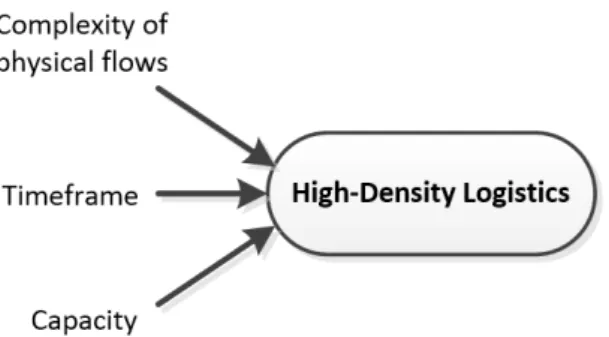
The Council of Supply Chain Management Professionals defines logistics management as “the part of supply chain management that plans, implements, and controls the efficient, effective forward and reverse flow and storage of goods, services and related information between the point of origin and the point of consumption in order to meet customers' requirements” (CSCMP, 2017). This definition emphasizes four aspects of logistics: (i) efficiency and effectiveness, (ii) physical flows, (iii) customer requirements, and (iv) information flows. In defining HDL, we connect the first three aspects to the three dimensions that characterize an HDL context. Then we propose the use of the fourth aspect, information flows, as a mean to tackle the logistics challenges caused by HDL. The dimensions in defining the HDL environment are shown in Figure 1 and elaborated in the following.

Figure 1. Three dimensions in defining high-density logistics

• Complexity of physical flows in the logistics process: a physical flow involves moving products between two points in the supply chain, which can be within a facility or between facilities. The complexity of physical flows in a logistics process can be influenced by the number of items that need to be handled throughout the logistics process (i.e. the number of physical flows) or by the number of material handling activities (i.e. the number of stages) in the process. For example, in the distribution process between a manufacturer and a retailer in the case studies by Liu et al. (2009) and Bryan and Srinivasan (2014), the flow complexity is influenced by the fact that a large number of shipments have to pass multiple facilities and stages before arriving at the retailer. Another example is the order-picking process in a distribution center in which the daily total number of orders, the number of order lines and stock keeping units (which are located in different picking zones) per order will affect the complexity of the process (Le-Duc, 2005). In these examples, increasing customer requirements on product variety (with small orders) is the main cause of increased complexity.

• Timeframe of the logistics process: this is defined by the time required to perform logistics activities, e.g. the timeframe of the distribution process is the required delivery lead time of an order. Time is one of the most important aspects in fast-moving consumer product chains and agro-food value chains (Brandenburg and Seuring, 2011). As these chains have become more demand-driven (Trienekens et al., 2003), customer requirements have also become stricter on delivery lead times to improve the chains’ competitive advantage (Morash et al., 1996).

• Capacity: the capacity of logistics resources utilized in a logistics process such as human resource, truck fleet size, and travelling space in the warehouses. Because the resources are limited and shared among different supply chain actors or different logistics processes (Arshinder et al., 2011), an efficient and effective capacity allocation is a determinant factor in the success of the logistics activities (Perona and Miragliotta, 2004).

Given a fixed capacity, a logistics process develops towards a high-density context if the timeframe becomes shorter or the complexity of physical flows becomes higher.

An example of an HDL context is city logistics distribution operations. Recently, many western European cities have applied strict regulations that force the distribution activities of retail chain to take place within a specific time period (Quak and de Koster, 2007). These regulations make the distribution

schedule from distribution centers to retail outlets more difficult because of the shorter time available for order processing and delivery, and increasing congestion because there are more trucks moving on city roads within the same time windows (Stathopoulos et al., 2012). At the same time, the size of retail order is decreasing, and subsequently, the number of handling and the physical flows in order processing (e.g., receiving, sorting, transferring, picking) at the distribution warehouse are increased (Quak and de Koster, 2009). In this example, HDL is caused by both a shorter timeframe and a higher complexity of physical flow.

The second example of HDL is the distribution in the Dutch floricultural sector. The supply chain network of the sector consists of approximately 5000 national and international growers; 1200 buyers, including wholesalers, exporters, importers; 70 logistics service providers; 6 auction sites and many market places. The consumers of flowers and ornamental plants have not only become more demanding with regard to product variety and availability at shops but also on product shelf life (van der Vorst et al., 2012; Verdouw et al., 2013). As a result, buyers place more small orders for a large variety of products every day (De Keizer et al., 2015). The average order size has dropped from full flower trolleys to less than a trolley (e.g. a number of buckets). From the point of view of auctions and distribution, this implies that a full flower trolley has to be split over several buyers; thus the number of handling operations and the complexity of logistics processes have increased significantly. Moreover, because the buyers demand products with a longer shelf life, shorter delivery lead times (i.e. between 2 and 4 hours) have become the “new normal” (Wallace and Xia, 2014). In this example, both dimensions have become more restricted (i.e. a shorter timeframe and a higher complexity of logistics and distribution processes), which makes the daily distribution in the Dutch sector very challenging. In Section 4, we specifically discuss the logistics challenges caused by HDL at the distribution warehouse for a Dutch flower supply chain.

Integrating information flows in decision-making can leverage the existing logistics resources to achieve the distribution challenge (Lee and Whang, 2001; Lumsden and Mirzabeiki, 2008). The Dutch floricultural sector is active in improving information sharing and information availability throughout the supply chain network (Verdouw et al., 2014a). Taking advantage of the rising momentum of information availability, we propose that the daily distribution process in the case study can be improved by using outbound and inbound information flows in operational planning. Outbound information includes order information such as required lead times, quantity, and destination for each consignment. Inbound information basically includes the contents of the inbound trucks. In addition, the growers can also share information on the arrival time of the inbound trucks with the warehouse operator. In the case study, we examine the value of both outbound and inbound information. Before introducing the case study and the use of inbound and outbound information in decision making, we provide the theoretical background on the VOI in supply chain and logistics decision making in the following section.

3

Value of Information in the Supply chain and Logistics

We first provide an overview of the literature on the VOI in decision making to improve logistics performance. Thereafter, we discuss a stepwise framework to evaluate the value of inbound and outbound information in the case study.

3.1 Value of information in supply chain and logistics decisions

VOI can be seen from two angles. The first associates VOI with the willingness of the information users to pay to gain access to the information (King and Griffiths, 1986). The second defines VOI as the resulting (or expected) benefits from using the information in making a specific decision (Lumsden and Mirzabeiki, 2008). The benefits are determined as improvements in one or several key performance indicators (KPIs) that are achieved through the use of the information in decision making compared with the base scenario in which the information does not exist (Ketzenberg et al., 2006; Ganesh et al., 2014). Therefore, a piece of information can have different values when it is used in different supply chain and logistics decisions. Here, we adopt the second approach, which is also the dominant view in the literature.

The largest part of the VOI literature is about the value of information sharing in inventory decisions such as decisions on order quantity, order frequency, safety stock, etc. The general conclusion from these studies is that the VOI is positive, yet numerically sensitive to logistics process parameters such as capacity, inventory costs, and lead time (Li et al., 2005). We refer to Ketzenberg et al. (2007) and Giard and Sali (2013) for extensive reviews on the value of information sharing in inventory decisions. The second largest area of the literature concerns the VOI in transportation decisions. In collaborative transporation, advanced load information from shippers enables carriers to better plan vehicle routing, and the pickup and delivery schedule (Tjokroamidjojo et al., 2006; Zolfagharinia and Haughton, 2014). Product location information enabled by tracking and tracing technologies is a highly demanded

information type by supply chain members (Lumsden and Mirzabeiki, 2008). This type of information is frequently used in optimizing transportation decisions, including vehicle routing and repositioning of empty vehicles (Kim et al., 2008; Flamini et al., 2011).

The literature focusing on the VOI to improve distribution and warehousing decisions is limited. The use of outbound information (i.e. order information) has been considered extensively in the order-picking literature (de Koster et al., 2007), whereas the literature on the value of inbound information, especially information on truck-arrival time, is rather scant. The reason is that most of the literature assumes that the truck contents and arrival time information are always available for solving distribution warehouse problems, such as inbound and outbound truck scheduling (Ladier and Alpan, 2016). In one of the few studies on this domain, Larbi et al. (2011) studied the VOI on inbound truck contents and arrival time to improve the scheduling of outbound trucks. In their study, three scenarios were explored: full information (i.e. every detail about inbound truck content and arrival time is known), partial information (i.e. contents and arrival times of a number of inbound trucks are known), and no information (i.e. no inbound information is available). The authors concluded that knowing the contents and arrival times of the next 14 inbound trucks is as valuable as knowing the arrival times of all the next trucks to arrive. However, their approaches use exact truck arrival time, which is hard to obtain; in reality, many factors such as traffic congestion can affect the truck arrival time. In addition to Larbi et al. (2011), who explicitly discuss the value of inbound information in managing warehouse operations, other studies have emphasized the importance of considering the uncertainty of truck-arrival time in solving the truck scheduling problem; see for example the study by Konur and Golias (2013).

An important factor in determining the VOI in logistics is the characteristics of the information. Most of the literature considers only the availability aspect of information. In other words, these studies compare two scenarios: decision making with- and without information. However, in many cases, not only the availability of information but also other information characteristics such as timeliness, accuracy, completeness, consistency, and security may influence the VOI. Information characteristics have also been addressed under two different terms: information quality dimension (Miller, 1996; Gustavsson and Wänström, 2009), or information value attributes (Sellitto et al., 2007; Leviäkangas, 2011). These terms are interchangeable from the perspective of their impact on the VOI. A recent extensive literature review on the VOI by Viet et al. (2017) reveals that the three intrinsic characteristics of information - accuracy, timeliness and completeness – have been studied the most. The definition of these characteristics is provided in Table 1. In the case study, we also focus on these three characteristics in the assessment of the VOI because they are objective to the information (Hazen et al., 2014).

Table 1.

Definitions of three intrinsic information characteristics

Characteristic Definition

Accuracy Accuracy defines how the available information reflects the underlying reality

Timeliness Timeliness indicates how up to date the information is and how well it meets the demand for information in a particular time and space.

Completeness Completeness refers to different levels of detail of the information.

3.2 Stepwise framework to assess the VOI

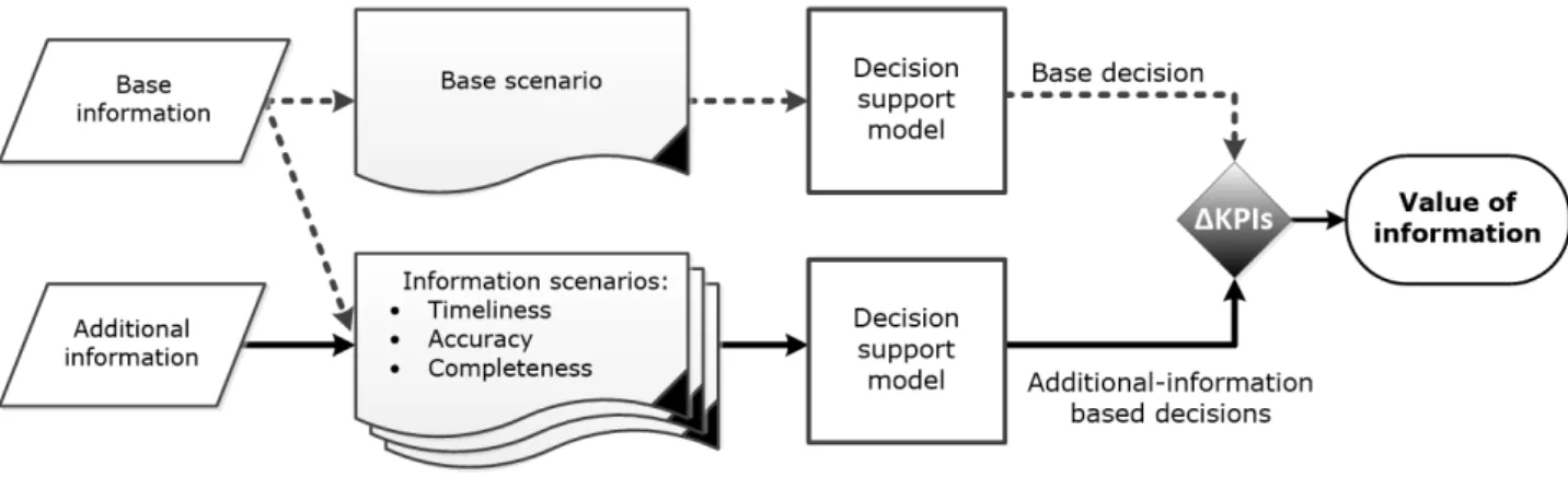
We follow the stepwise framework on assessing the VOI in supply chain and logistics decisions as proposed by Viet et al. (2017). As depicted in Figure 2, the VOI is assessed by comparing the KPIs resulting from two decision-making scenarios:

• In the base scenario, base information is used. Base information is a given set of information (with some specific information characteristics) that is available originally to the decision maker. Accordingly, the base decision is the output from the decision-support model using this base information. In some cases, no information is used in the base scenario.

• In the information scenario, additional information is added to the base information. The additional information is expected to contribute to an improvement in the logistics performance. The decision maker aims to assess the value of this additional information. Given the additional and the base information as input, the decision-support model generates the decision based on the additional

information as output. The difference between performance measures in this case and the base scenario determines the VOI. Furthermore, multiple information sub-scenarios can be defined by considering different options for different information characteristics. Studying these sub-scenarios will provide insight into the impact of the information characteristics on the VOI. The results of this analysis can be used to determine the requirements for information characteristics in information sharing between different actors in the chain.

In the framework, different decision-support models can be used in the base and information scenarios. For instance, in the study by Larbi et al. (2011), a polynomial algorithm is developed for full information scenarios and two heuristics are used for the partial and no information scenarios. In the next section we apply this framework to the case study.

Figure 2. Stepwise framework to assess the VOI in improving the logistics performance

4

A Case Study on a Dutch Flower Supply Chain

In this section, we elaborate on the current HDL situation at the distribution warehouse of a Dutch flower supply chain and the scope of this study. Subsequently, we discuss how the value of inbound and outbound information can be assessed by mapping each concept in the research framework to the case study.

4.1 Case description

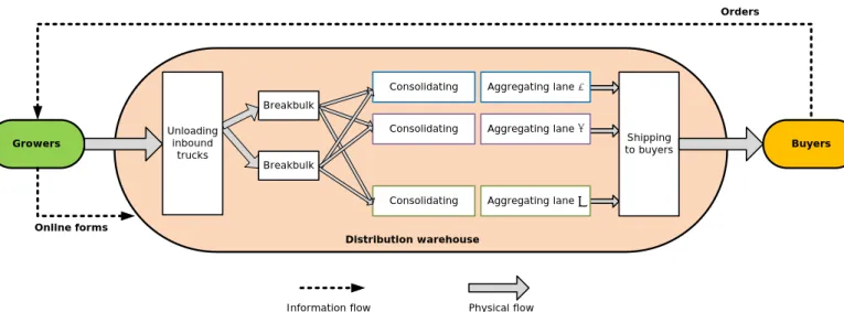
The distribution warehouse in this case study is part of a Dutch flower supply chain. The flower growers send the flower orders by trucks to the warehouse, and the warehouse is responsible for distributing the right flowers to the right buyers in the right quantities. The buyers’ facilities are in the neighborhood surrounding the warehouse. Figure 3 shows the information flows and the physical flows in the supply chain.

4.1.1 Information flows

After processing the orders from the buyers received in a day, growers send online forms to the distribution warehouse indicating the destination of each flower bucket in the flower trolleys that will be transported by trucks to the warehouse. Regularly, the warehouse receives the forms the night before the flower trolleys arrive. Urgent orders, which require lead times of around two hours, are not considered in this study because the growers often send flowers for urgent orders directly to the buyers’ facilities. In addition, currently information on the truck arrival time is not included in the online forms. We design multiple scenarios about the availability of truck arrival time information in the experiment section.

Figure 3. Information flows and physical flows in the Dutch flower supply chain

4.1.2 Physical flows

At the grower sites, many buckets of the same type flower are consolidated to make full trolleys. Each trolley can contain a maximum of 30 buckets. The inbound trucks transporting the trolleys usually arrive at the warehouse from 9:00 hours in the morning. The trucks are unloaded on a first-come first-serve policy. As shown in Figure 3, the internal process at the warehouse between unloading and shipping consists of three stages: breakbulk, consolidating, and aggregating. All unloaded flower trolleys are queued at the breakbulk area, with a first-in first-out policy. Next to the breakbulk area are multiple parallel consolidating and aggregating lanes. Each lane is reserved for a buyer, or a group of buyers whose facilities are closely located to each other. Empty trolleys are prepared at the lanes to receive flower buckets from the breakbulk area.

From the breakbulk area, flower trolleys are distributed to the consolidating and aggregating lanes following the “put system” order-picking (de Koster et al., 2007), which is a popular method for floricultural products and for distribution systems with a large number of orders and a short time window for picking. A worker can carry a trolley directly to a consolidating and aggregating lane if all the buckets in the trolley are to be distributed to the same destination. This happens when the order quantity is large enough. Otherwise, the workers have to drive the trolley to multiple consolidating and aggregating lanes and place the correct number of (ordered) buckets in the trolleys waiting at the lanes. Currently, on average, 60% of inbound trolleys are split among multiple buyers’ lanes due to the high number of small order quantities and the high number of flower varieties. As a consequence, the average time for processing an inbound trolley has increased. The number and complexity of the physical flows has also increased because the worker has to move a trolley multiple times. As a result, congestion often occurs in the travelling space between the breakbulk and the consolidating and aggregating areas. Here we define

the variable β as “the percentage of inbound trolleys that are not split at breakbulk stage”; so in the base

case, β is equal to 40%. Later this variable will be varied to model different levels of high-density in the

distribution process. The lower β is, the higher the complexity of the physical flows, and thus the higher

the density level.

At each consolidating and aggregating lane, flower buckets are merged into full trolleys again. Full trolleys are aggregated and physically connected before they are shipped to the buyers. Currently one worker is in charge of a number of lanes. The worker waits until an aggregating lane reaches 12 trolleys, which is the maximum size, and then ships the set of aggregated trolleys to their destination. It takes a worker on average 15 minutes to drive the aggregated set to the buyers’ facilities. Larger aggregating sizes require longer shipping time.

At the buyers’ facilities, trolleys are then re-processed for deliveries to their next customers. The buyers place high value on deliveries within a 4-hour time window from 9:00 to 13:00 hours which provides sufficient time for their internal logistics activities. We specify this “time window” as Ƭ (hours). In the experimental design, Ƭ is varied to demonstrate different levels of density. The lower Ƭ is, the higher the density level.

Consolidating Consolidating

Consolidating Aggregating lane 1

Aggregating lane 2

Aggregating lane n

Shipping to buyers

Growers

Breakbulk

Breakbulk

Buyers

Distribution warehouse

Orders

Online forms

Unloading inbound

trucks

4.1.3 Scope of this study

In the current situation, the warehouse distributes flowers to a large number of buyers. In the case study, we simplify the current warehouse situation by modelling only three consolidating and aggregating lanes (three groups of buyers). This simplification is justified because we aim for an illustrative case to study the HDL context and the VOI. Therefore, the VOI could be higher in the real situation with the entire distribution system. In addition, we assume a fixed time period for unloading each inbound truck. Our focus is on the complexity of the operations in the three internal stages: breakbulk, consolidating, and aggregating. Two workers work at the breakbulk, consolidating, and aggregating areas. One worker waits at the three aggregating lanes. The day shift of the workers ends when all the inbound trolleys have been processed and delivered.

4.2 Applying the VOI assessment framework to the case study

In this case study, we aim to evaluate the value of inbound and outbound information in improving the logistics performance at the warehouse. Specifically, inbound information is the truck-arrival time information, and outbound information is the order information. Ketzenberg et al. (2007) conclude that the value of additional information depends on the base information in the base scenario. The more information types used in the current decision-making, the lower the value of the additional information can be. Currently, outbound information is available at the warehouse but unused. To understand the value of the outbound and inbound information, we consider three scenarios:

(i) Base scenario: no information is used in decision-making as in the current situation; (ii) Outbound information scenario: only outbound information is used; and

(iii) Total information scenario: both outbound and inbound information is used.

In the following, we first define the logistics KPI and the planning decision. Subsequently, we discuss the mapping of each concept in the VOI framework to the case study in each scenario.

• KPIs: The first indicator KPI1 is defined as the number of full trolleys that are distributed to the buyers before the time window Ƭ. The travelling cost at the shipping stage is mainly associated with the utilization of the shipping workers, which is insignificant in this case. The second indicator KPI2 is the completion time to deliver all the inbound trolleys to the buyers. To quantify the VOI, we used the total improvement in these KPIs where the KPIs are equally important:

(1) • The decision: Truck-arrival time information is used to schedule outbound trucks in Larbi et al. (2011)

and Amini et al. (2014). In this case study, we scheduled the outbound shipping trips by dynamically changing the aggregating sizes at each aggregating lane because the aggregating sizes directly affect both KPIs. Dynamically updating the aggregating sizes every hour can reduce a worker’s productivity. In this case study, we aim to locate the aggregating sizes of the lanes before and after the time window Ƭ for future practical implementation.

From the scheduling problem perspective, the problem in this case study falls into the category of a single batch-process machine with dynamic job arrivals. Full trolleys at the aggregating lanes that need to be shipped can be seen as jobs, the single machine is the worker, the batch service time is the shipping time of the set of aggregated trolleys, and the decision variable is the batch size, i.e. the aggregating size. This type of scheduling problem has been studied extensively in the literature (Ikura and Gimple, 1986; Lee and Uzsoy, 1999). The classic problem formulation is “given n jobs Ji with release times ri (i = 1, 2, …, n) and batch service time µ independent of batch size, minimize the completion time”. In this case study, the problem setting is slightly different because in addition to the completion time KPI2, the number of full trolleys distributed to the buyers before the time window Ƭ (KPI1) must also be considered. Moreover, the batch service time depends on the batch size. Therefore, we formulate the problem as “given n jobs Ji

with release times ri (i = 1, 2, …, n) and batch service time µs (which depends on batch size s),

maximize QƬ and minimize the completion time; where QƬ is the number of jobs finished before time

Ƭ”. Moreover, the release time ri, i.e., the time when a trolley at the aggregating lane is ready for shipping, is unknown. We explain the method to estimate the release time ri using the information in each

information scenario.

4.2.1 Base scenario

• Base information: in the base scenario, which represents the current situation, no information is used in the decision making. The shipping worker waits until an aggregating lane reaches 12 trolleys. In this case, the aggregating size combination is (12, 12, 12) for three lanes.

• Decision-support model is not needed in this base scenario.

4.2.2 Outbound information scenario

• Additional information: order information

• Decision-support model – a scheduling algorithm: we developed a polynomial time scheduling algorithm based on the order information. Without the truck arrival time, the objective of the algorithm is solely to improve KPI2, the completion time. Two main inputs for the algorithm are (i) the total trolley quantity ordered for each aggregating lane and (ii) the estimated time interval for a trolley to be fully filled with flower buckets at the aggregating lanes (i.e. the inter-arrival of the release time ri ). The total trolley quantity ordered can be easily calculated from the order information. The second input is estimated based on the average deterministic flow time at the breakbulk and consolidating stages, similar to the common practice of modelling warehouse handling in the literature (Boysen et al., 2010; Konur and Golias, 2013). With the two inputs, the algorithm can calculate the completion time for each aggregating size combination. The algorithm loops exhaustively through all the combinations of the aggregating sizes and selects the one with the shortest completion time. The pseudo-code is provided in Appendix A.

• Information characteristics: we assume that the order information is accurate, complete and available at the moment of decision-making.

4.2.3 Total information scenario

• Additional information: both the truck-arrival time information and the order information

• Decision-support model – a simulation-based scheduling algorithm: knowing the truck arrival time information, the time that the inbound trolleys enter the internal process is known. The dynamic operations at the breakbulk and consolidating stages cannot be modelled by queueing systems. To estimate the release time ri, we built a discrete-event simulation model that includes only the breakbulk and consolidating stages (i.e. a partial simulation model) using the Enterprise Dynamics 9 software package (EnterpriseDynamics, 2017). Discrete-event simulation is widely used for modelling logistics operation processes (Tako and Robinson, 2012). Given the truck arrival time information and order information, the partial simulation model records the release time ri of each full trolley at each aggregating lane. Because the simulation model uses stochastic cycle times of worker operations at the breakbulk and consolidating stages (Appendix B), the recorded release time ri are different for different simulation runs. However, the recorded release time ri from a single run is an acceptable estimation because we do not need the exact release time of each job arrival, but the estimated release time of an s-sizedbatch of jobs; i.e. the time that a s-sized set of aggregated trolleys is ready for shipping.

Using the recorded release time ri as input, we developed a similar scheduling algorithm to the one in the outbound information scenario. The algorithm loops exhaustively for the entire set of aggregating size combinations. Before the time window Ƭ, the algorithm selects the combination with the highest KPI1, the number of trolleys delivered within the time window Ƭ. After the time window Ƭ, it selects the combination with the shortest KPI2, completion time of the remained trolleys. The pseudo-code is provided in Appendix C.

• Information characteristics: each information characteristic needs specific interpretation according to the specific logistics context. In this case study, we interpreted the characteristics as follows and explain why the focus is on information accuracy.

 Information accuracy: the inbound information is inaccurate if the trucks actually arrive earlier or later than the arrival time provided.

 Information completeness: with regard to the level of detail for inbound truck arrival information, it is common in practice that, instead of an exact time, a time window in quarter hours is provided for each truck (Konur and Golias, 2013). In other words, the lower and upper bounds of a truck’s arrival time are known. For example, the information states that truck A will arrive in one-quarter time window between 9:00 and 9:15 hours, and truck B will

arrive in a two-quarter time window between 9:00 and 9:30 hours. In these cases, the warehouse operator can use the mid-arrival time windows in his scheduling as suggested by Konur andGolias (2013): truck A is expected to arrive at 9:07:30 hours, and 9:15:00 hours for truck B. Therefore, we associate the impact of information completeness with the impact of information accuracy by investigating the impact of information accuracy in different ranges of inaccuracy.

 Information timeliness: from the time dimension, the information is considered timely if it arrives before the warehouse operator makes the schedule. Because this case study does not include the urgent orders, we assume that the growers will have sufficient time to provide the truck arrival information on the online forms.

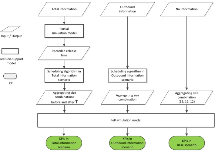
4.2.4 Summary of decision-making flows in the three scenarios

For a fair comparison of the KPIs in all three scenarios, the output aggregating size combinations in these scenarios need to be examined by the same tool and in a stochastic environment to reflect the dynamic nature of warehouse operations. The partial discrete-event simulation was extended to include the complete distribution process i.e. full simulation model. Figure 4 summarizes the decision-making flows in the three scenarios.

Figure 4. Decision-making flows in the three scenarios

4.3 Experimental design and results

We designed different sets of experiments to test the VOI in different parameter settings, in different density levels, and in different scenarios of information accuracy. In each set of experiments, one parameter is varied while the others are fixed at the values in the current situation. Because of the stochastic nature of the parameters in the simulation model, it is incorrect to measure the VOI based on the KPIs observed from a single run. Therefore, we executed 50 separate runs for each parametric setting to achieve narrow intervals with a 95% confidence level. In this way, the mean KPIs obtained from the 50 runs could be used to calculate the VOI. The experiments and the results are elaborated in the following. Input / Output

Decision-support model

KPI

Aggregating size combinations before and after Ƭ

Aggregating size combination

Aggregating size combination

(12, 12, 12)

Full simulation model

KPIs in Total information

scenario

KPIs in Outbound information

scenario

KPIs in Base scenario Scheduling algorithm in

Total information scenario

Scheduling algorithm in Outbound information

scenario Recorded release

time

Partial simulation model

Partial simulation model

4.3.1 Value of accurate information

We investigate the VOI assuming that accurate order information and accurate and exact arrival times of all the trucks are provided. The VOI is subject to logistics process parameters (Li et al., 2005). To carry out the sensitivity experiments, we generated five different datasets based on five different means of the inbound truck inter-arrival time, as shown in Table 2. The bold values indicate the current situation. The current literature has not considered truck inter-arrival time when assessing the value of truck-arrival time information in truck scheduling. We aim to test if the truck inter-arrival time can be an influential factor on the internal handling operations and the value of order and truck-arrival time information.

Table 2.

Parameter setting in experiments on the inter-arrival time of inbound trucks

Parameter Value

Inter-arrival time of trucks Exponential distribution with mean: 6, 8, 10, 12, 15 minutes

β 40%

Time window Ƭ 4 hours

In the five sensitivity experiments, the inter-arrival times of 30 trucks were randomly generated using exponential distribution with different means when the trucks’ contents, i.e. β, and time window Ƭ were unchanged. Each truck carries between 8 and 12 full trolleys. For each full trolley, the allocation of flower buckets to three buyer destinations was randomized using uniform distribution, yet the sum of the quantities was always 30. Currently 40% of the inbound trolleys are fully ordered by one buyer destination (β = 40%); in this case, the possible quantity combinations are (30, 0, 0) or (0, 30, 0) or (0, 0, 30). Details of the other parameters, such as the cycle times at breakbulk, consolidating, and aggregating stages are provided in Appendix B.

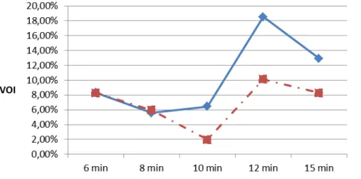
Figure 5. VOI with different means of truck inter-arrival time

The value of outbound information (VOIoutbound) and the value of total information (VOItotal) are positive as shown in Figure 5. The VOI is the percentage improvement in KPIs compared with the base scenario, as presented in Equation 1. The numerical values vary between 1.99% and 10.11% for VOIoutbound, and between 5.57% and 18.52% for VOItotal. We observe that the VOItotal is generally higher than the VOIoutbound. This result supports the conclusion by Ketzenberg et al. (2007) and Ketzenberg et al. (2006): using an additional information type results in additional benefit. In this case, inbound information adds additional value on top of the outbound information. However, this conclusion is not always true.

Interested readers are referred to the results of the case study by Rached et al. (2015) and the analysis on this issue by Viet et al. (2017).

Furthermore, we observed no clear relationship between the VOIoutbound and the truck inter-arrival time means, which is intuitive. However, the gap between VOItotal and VOIoutbound increases as the mean inter-arrival time becomes larger. This gap can be interpreted as the additional value from the truck inter-arrival time information, inbound information. We define VOIinbound as the additional value of the inbound truck arrival time information, given that the order information is already in use in decision making. We measured VOIinbound in Equation 2 by comparing the KPIs in the total information scenario with those in the outbound information scenario. In other words, the outbound information scenario serves as the base scenario in assessing the VOIinbound.

(2)

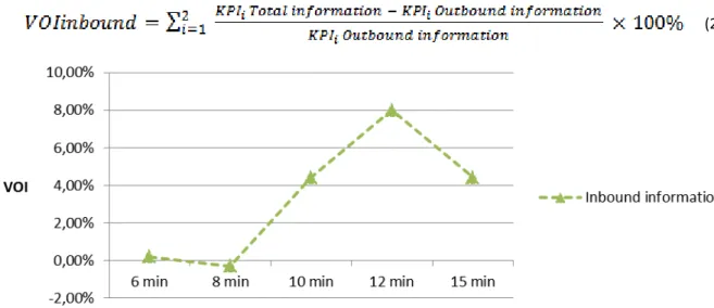
Figure 6. VOIinbound with different means of truck inter-arrival time

Figure 6 reports the numerical values of VOIinbound in the five experiments on inbound truck inter-arrival times. In the cases of 6 minutes and 8 minutes, the VOIinbound is close to zero (0.20% and 0.30%, respectively). The VOIinbound is higher when the inter-arrival time mean is larger. This observation implies that the additional information does not always result in additional value in some specific contexts (in this case, for the small value of the mean truck inter-arrival time). We suggest that the VOIinbound is small with the small mean inter-arrival times because the observed deterministic flow time of the breakbulk and consolidating stages in the outbound information scenario performs well with small inter-arrival time. As a result, the difference between the KPIs in total information scenario and outbound information scenario is small, thus VOIinbound is small. As the mean inter-arrival time becomes larger, the flow time, especially at the consolidating stage, fluctuates more widely. Therefore, the deterministic value cannot be representative for the dynamic flow time of products through the stages.

4.3.2 Value of accurate information for different density levels

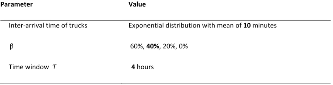
We measured the VOI at different levels of density by changing the value of the time window Ƭ and the

value of β.

4.3.2.1 Time window Ƭ: timeframe of the logistics process

By varying Ƭ, the timeframe of the logistics process is changed. The smaller Ƭ is, the higher the density level. In the experiments on Ƭ, the truck-arrival times and the truck contents were unchanged, as shown in Table 3.

Table 3.

Parameter setting in experiments on time window Ƭ

Parameter Value

Inter-arrival time of trucks Exponential distribution with mean of 10 minutes

β 40%

Time window Ƭ 5, 4, 3, 2 hours

Figure 7 illustrates the results. On the timeframe dimension, the VOIoutbound (and thus VOItotal also) increases as the density level increases. Also, one can see that as the timeframe of the process is long enough, these two VOIs converge to zero (at 5 hours) because the combination of maximum aggregating sizes (12, 12, 12) for the base scenario performs well with long timeframes as suggested by Ikura and Gimple (1986). Contradictorily, the VOIinbound peaks at Ƭ = 4 hours and then decreases as the density level increases; at Ƭ = 2 hours, the VOIinbound is approximately equal to zero.

Figure 7. VOI with different settings for time window Ƭ

4.3.2.2 β: the complexity of physical flow

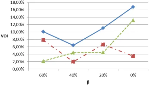
By varying β, the complexity of the physical flow is altered. The lower β is (i.e. the more trolleys are split

over multiple buyer destinations), the higher the complexity, and thus the higher the density level. In the

experiments on β, the truck arrival times and the time window Ƭ were unchanged, whereas the allocation

of flower bucket quantities to each buyer destinations was done according to different values of β, as

shown in Table 4.

Table 4. Parameter Setting In Experiments On β

Parameter Value

Inter-arrival time of trucks Exponential distribution with mean of 10 minutes

β 60%, 40%, 20%, 0%

Figure 8 shows the results. On the complexity of the physical flows dimension, the VOIinbound increases as the density level increases, whereas the VOIoutbound does not have a clear relationship with the density level. As a result of increasing VOIinbound, the VOItotal also increases.

Figure 8. VOI with different settings for β

4.3.3 Summary on the value of accurate information

The impact of process parameters on the values for inbound, outbound, and total information are summarized in Table 5. Overall, the results of the experiments point to (i) a positive correlation between the VOIinbound and the mean inbound truck inter-arrival time, (ii) a positive correlation between the VOIinbound/VOItotal and the density level on the physical flow complexity dimension, and (iii) a positive correlation between the VOIoutbound/VOItotal and the density level on the timeframe dimension. Understanding the impact of the parameters on VOI, especially the parameters that affect the dimensions of HDL, improves the decision about which information to collect and use in different characteristics of the HDL processes.

Table 5.

Summary on value of accurate information

VOI

Impact of process parameter Mean truck

inter-arrival time

Density level on timeframe dimension

Density level on physical flow complexity dimension

Value of outbound

information Non-monotonic Positively correlated Non-monotonic

Value of inbound

information Positively correlated Non-monotonic Positively correlated

4.3.4 Impact of inaccurate information

In the previous experiments, we assumed that the information was accurate. Now, we consider inaccurate truck-arrival time information and examine how information accuracy influences the VOIinbound. Three scenarios of information accuracy were established by adding random errors to the exact truck arrival times. The mean of truck inter-arrival time was kept at 10 minutes as in the current situation. In detail, suppose ti (i = 1, 2, ..., 30) are the accurate truck-arrival times, the inaccurate truck-arrival times are ti +

εi (i = 1, 2, …, 30) where εi are the randomized integers following uniform distributions with three

different intervals: (-7,7) minutes, (-15,15) minutes, and (-30,30) minutes. These three intervals link to three inbound trucks’ arrival time windows of one-, two-, and four quarters of an hour, respectively (Konur and Golias, 2013). With each error interval, we randomized two different data sets. In each scenario, we input the full simulation model with the inaccurate truck-arrival times, yet with the same aggregating size combinations obtained from the decision making based on the accurate information scenario. The purpose is to examine how the decisions based on the accurate truck-arrival time information perform in the case of inaccurate truck arrival times.

The results of experiments on inaccurate information are shown in Table 6. Intuitively we would expect that inaccurate information would reduce the VOI. The results support the expectation, yet it is not clear if there is a relationship between the magnitude of reduction and the error interval. Generally, the VOIinbound remains positive in most of the experiments except one case in the error interval of (-15, 15).

Table 6.

Results of the experiments on inaccurate information

Error interval (minutes) Truck-arrival information VOIinbound

0 Accurate information 4.42%

(-7,7) Inaccurate information dataset 1 2.10%

(-7,7) Inaccurate information dataset 2 1.80%

(-15,15) Inaccurate information dataset 1 -2.08%

(-15,15) Inaccurate information dataset 2 3.46%

(-30,30) Inaccurate information dataset 1 3.31%

(-30,30) Inaccurate information dataset 2 4.16%

5

Discussion and Conclusion

This paper discusses the HDL context in agro-food supply chains in which the distribution process is confronted with more frequent small orders and short lead times. The capacity of logistics resources, the expected timeframe of logistics activities, and the complexity of physical flows in a logistics process are the main factors that shape HDL. The concept is further elaborated through a case study on the distribution warehouse of a Dutch floricultural supply chain. We further discuss the value of inbound and outbound information to improve the logistics performance in the HDL context. We find that as the density of the logistics context increases, the VOI increases. We also discuss the impact of information characteristics on the VOI; we particularly examine information accuracy and find that inaccurate truck-arrival information diminishes its value.

This research contributes to agro-food logistics by explicitly characterizing the HDL in agro-food supply chains, which is mainly caused by the increasing development from supply-driven towards demand-driven requirements. As proposed, effective uses of information flows are the key to overcome the logistics challenges. Extensive research is available on tackling technical challenges of virtual supply chains and smart systems of tracking, tracing, and sensing devices (Verdouw et al., 2013; Verdouw et al., 2016; Wolfert et al., 2017). However, effective real-time uses of different information types enabled by such systems and virtualization in supply chain and logistics decisions remains a promising research area. For example, under regulations on food traceability, the availability of product location and condition information has been improved in the agro-food sector (Heyder et al., 2010; Bosona and Gebresenbet, 2013). Besides direct uses in relation to food safety, quality and food waste, this information can be useful in handling and distribution planning.

Decision-support models developed in the case study can be applied in operations planning at cross-docking distribution warehouses for fresh agricultural products. Particularly, the simulation-based scheduling approach in the total information scenario is suitable to capture dynamics and complex operations in the distribution process. For future research, we suggest two directions to extend the models. Firstly, we only discussed the use of inbound and outbound information in the outbound shipping scheduling decision. This information could have additional value if used in other decisions such as dynamic work force scheduling. We can model the dynamic work shifts of workers by varying the cycle time at each stage in the simulation. Another interesting direction is to include urgent orders in the scheduling process. Entering of flower trolleys linked to urgent orders into the internal distribution process can immediately trigger outbound shipping regardless of the current number of trolleys at the aggregating lanes; thus, it can affect the KPIs and the original shipping planning. Furthermore, the distribution network could be redesigned to be able to handle the distributions of different order types with different required lead times. In that case, we anticipate that the inbound information flows will play a more crucial role in efficient process coordination and resources allocation across the entire network.

Acknowledgements

This study was funded by the Top Kennis Instituut Tuinbouw en Uitgangsmaterialen, the Productschap Tuinbouw, and the participating companies.

References

Akkerman, R., Farahani, P., and Grunow, M. (2010). Quality, safety and sustainability in food distribution: a review of quantitative operations management approaches and challenges. Or Spectrum, 32(4): 863-904. doi: 10.1007/s00291-010-0223-2

Amini, A., Tavakkoli-Moghaddam, R., and Omidvar, A. (2014). Cross-docking truck scheduling with the arrival times for inbound trucks and the learning effect for unloading/loading processes. Production and Manufacturing Research, 2(1): 784-804. doi: 10.1080/21693277.2014.955217

Arshinder, K., Kanda, A., and Deshmukh, S. G. (2011). A review on supply chain coordination: coordination mechanisms, managing uncertainty and research directions. In T.-M. Choi & E. T. C. Cheng (Eds.), Supply Chain Coordination under Uncertainty (pp. 39-82): Springer Berlin Heidelberg.

Bosona, T., Gebresenbet, G. (2013). Food traceability as an integral part of logistics management in food and agricultural supply chain. Food Control, 33(1): 32-48. doi: 10.1016/j.foodcont.2013.02.004

Boysen, N., Fliedner, M., and Scholl, A. (2010). Scheduling inbound and outbound trucks at cross docking terminals. Or Spectrum, 32(1): 135-161. doi: 10.1007/s00291-008-0139-2

Brandenburg, M., Seuring, S. (2011). Impacts of supply chain management on company value: benchmarking companies from the fast moving consumer goods industry. Logistics Research, 3(4): 233-248.

Bryan, N., Srinivasan, M. M. (2014). Real-time order tracking for supply systems with multiple transportation stages. European Journal of Operational Research, 236(2): 548-560. doi: 10.1016/j.ejor.2014.01.062

CSCMP. (2017). CSCMP Glossary. Retrieved 16 May 2017, from http://cscmp.org/CSCMP/Educate/SCM_Definitions_and_Glossary_of_Terms/CSCMP/Educate/SCM_Defini tions_and_Glossary_of_Terms.aspx?hkey=60879588-f65f-4ab5-8c4b-6878815ef921

De Keizer, M., Van Der Vorst, J. G. A. J., Bloemhof, J. M., and Haijema, R. (2015). Floricultural supply chain network design and control: industry needs and modelling challenges. Journal on Chain and Network Science, 15(1): 61-81. doi: 10.3920/jcns2014.0001

de Koster, R., Le-Duc, T., and Roodbergen, K. J. (2007). Design and control of warehouse order picking: a literature review. European Journal of Operational Research, 182(2): 481-501. doi: 10.1016/j.ejor.2006.07.009

EnterpriseDynamics. (2017). Enterprise Dynamics 9. Retrieved 14 January 2017 http://www.incontrolsim.com/product/enterprise-dynamics/

Fernie, J., Sparks, L. (2014). Logistics and retail management: emerging issues and new challenges in the retail supply chain (4th ed.). London: Kogan Page Publishers.

Flamini, M., Nigro, M., and Pacciarelli, D. (2011). Assessing the value of information for retail distribution of perishable goods. European Transport Research Review, 3(2): 103-112. doi: 10.1007/s12544-011-0051-8 FMI. (2010). Food retailing industry speaks 2010 Arlington, VA: Food Marketing Institute.

Ganesh, M., Raghunathan, S., and Rajendran, C. (2014). The value of information sharing in a multi-product, multi-level supply chain: impact of product substitution, demand correlation, and partial information sharing. Decision Support Systems, 58(1): 79-94. doi: 10.1016/j.dss.2013.01.012

Giard, V., Sali, M. (2013). The bullwhip effect in supply chains: a study of contingent and incomplete literature.

International Journal of Production Research, 51(13): 3880-3893. doi: 10.1080/00207543.2012.754552 Gustavsson, M., Wänström, C. (2009). Assessing information quality in manufacturing planning and control

processes. International Journal of Quality and Reliability Management, 26(4): 325-340.

Hazen, B. T., Boone, C. A., Ezell, J. D., and Jones-Farmer, L. A. (2014). Data quality for data science, predictive analytics, and big data in supply chain management: an introduction to the problem and suggestions for research and applications. International Journal of Production Economics, 154: 72-80. doi: 10.1016/j.ijpe.2014.04.018

Heyder, M., Hollmann-Hespos, T., and Theuvsen, L. (2010). Agribusiness firm reactions to regulations: the case of investments in traceability systems. International journal on food system dynamics, 1(2): 133-142. Ikura, Y., Gimple, M. (1986). Efficient scheduling algorithms for a single batch processing machine. Operations

Research Letters, 5(2): 61-65. doi: 10.1016/0167-6377(86)90104-5

Ketzenberg, M. E., Rosenzweig, E. D., Marucheck, A. E., and Metters, R. D. (2007). A framework for the value of information in inventory replenishment. European Journal of Operational Research, 182(3): 1230-1250. doi: 10.1016/j.ejor.2006.09.044

Ketzenberg, M. E., Van Der Laan, E., and Teunter, R. H. (2006). Value of information in closed loop supply chains. Production and Operations Management, 15(3): 393-406.

Kim, J., Tang, K., Kumara, S., Yee, S. T., and Tew, J. (2008). Value analysis of location-enabled radio-frequency identification information on delivery chain performance. International Journal of Production Economics,

112(1): 403-415. doi: 10.1016/j.ijpe.2007.04.006

King, D., Griffiths, J. (1986). Measuring the value of information and information systems, services and products.

Paper presented at the AGARD Conference Proceedings.

Konur, D., Golias, M. M. (2013). Analysis of different approaches to cross-dock truck scheduling with truck arrival time uncertainty. Computers and Industrial Engineering, 65(4): 663-672. doi: 10.1016/j.cie.2013.05.009

Ladier, A. L., Alpan, G. (2016). Cross-docking operations: current research versus industry practice. Omega (United Kingdom),62: 145-162. doi: 10.1016/j.omega.2015.09.006

Larbi, R., Alpan, G., Baptiste, P., and Penz, B. (2011). Scheduling cross docking operations under full, partial and no information on inbound arrivals. Computers and Operations Research, 38(6): 889-900. doi: 10.1016/j.cor.2010.10.003

Le-Duc, T. (2005). Design and control of efficient order picking processes: Erasmus Research Institute of Management (ERIM).

Lee, C. Y., and Uzsoy, R. (1999). Minimizing makespan on a single batch processing machine with dynamic job arrivals. International Journal of Production Research,37(1): 219-236.

Lee, H. L., Whang, S. (2001). Winning the last mile of e-commerce. MIT Sloan Management Review, 42(4): 54. Leviäkangas, P. (2011). Building value in ITS services by analysing information service supply chains and value

attributes. International Journal of Intelligent Transportation Systems Research, 9(2): 47-54. doi: 10.1007/s13177-011-0029-x

Li, G., Yan, H., Wang, S. Y., and Xia, Y. S. (2005). Comparative analysis on value of information sharing in supply chains. Supply Chain Management-an International Journal, 10(1): 34-46. doi: 10.1108/13598540510578360

Liu, M., Srinivasan, M. M., and Vepkhvadze, N. (2009). What is the value of real-time shipment tracking information? IIE Transactions (Institute of Industrial Engineers), 41(12): 1019-1034. doi: 10.1080/07408170902906001

Lumsden, K., Mirzabeiki, V. (2008). Determining the value of information for different partners in the supply chain. International Journal of Physical Distribution & Logistics Management, 38(9): 659-673. doi: 10.1108/09600030810925953

Miller, H. (1996). The multiple dimensions of information quality. Information Systems Management, 13(2): 79-82. doi: 10.1080/10580539608906992

Morash, E. A., Droge, C. L., and Vickery, S. K. (1996). Strategic logistics capabilities for competitive advantage and firm success. Journal of Business Logistics, 17(1): 1.

Perona, M., Miragliotta, G. (2004). Complexity management and supply chain performance assessment. A field study and a conceptual framework. International Journal of Production Economics, 90(1): 103-115. doi: 10.1016/s0925-5273(02)00482-6

Quak, H., de Koster, M. B. (2009). Delivering goods in urban areas: how to deal with urban policy restrictions and the environment. Transportation Science, 43(2): 211-227.

Quak, H. J., de Koster, M. B. M. (2007). Exploring retailers’ sensitivity to local sustainability policies. Journal of Operations Management, 25(6): 1103-1122. doi: http://doi.org/10.1016/j.jom.2007.01.020

Rached, M., Bahroun, Z., and Campagne, J. P. (2015). Assessing the value of information sharing and its impact on the performance of the various partners in supply chains. Computers and Industrial Engineering, 88: 237-253. doi: 10.1016/j.cie.2015.07.007

Romsdal, A., Strandhagen, J. O., and Dreyer, H. C. (2014). Can differentiated production planning and control enable both responsiveness and efficiency in food production? International Journal on Food System Dynamics, 5(1): 34-43.

Sellitto, C., Burgess, S., and Hawking, P. (2007). Information quality attributes associated with RFID-derived benefits in the retail supply chain. International Journal of Retail and Distribution Management, 35(1): 69-87. doi: 10.1108/09590550710722350

Stathopoulos, A., Valeri, E., and Marcucci, E. (2012). Stakeholder reactions to urban freight policy innovation.

Journal of Transport Geography, 22: 34-45. doi: https://doi.org/10.1016/j.jtrangeo.2011.11.017

Tako, A. A., Robinson, S. (2012). The application of discrete event simulation and system dynamics in the logistics and supply chain context. Decision Support Systems, 52(4): 802-815. doi: http://dx.doi.org/10.1016/j.dss.2011.11.015

Tjokroamidjojo, D., Kutanoglu, E., and Taylor, G. D. (2006). Quantifying the value of advance load information in truckload trucking. Transportation Research Part E: Logistics and Transportation Review, 42(4): 340-357. doi: http://dx.doi.org/10.1016/j.tre.2005.01.001

Trienekens, J. H., Beulens, A., Hagen, J., and Omta, S. (2003). Innovation through (international) food supply chain development: a research agenda. International Food and Agribusiness Management Review, 6(1): -. Trienekens, J. H., van der Vorst, J. G. A. J., and Verdouw, C. N. (2014). Global food supply chains. In N. K. V.

Alfen (Ed.), Encyclopedia of Agriculture and Food Systems: 499-517. Oxford: Academic Press.

van der Vorst, J. G., Bloemhof, J. M., and de Keizer, M. (2012). Innovative logistics concepts in the floriculture sector. Proceedings in Food System Dynamics: 241-251.

van der Vorst, J. G., van Kooten, O., and Luning, P. A. (2011). Towards a diagnostic instrument to identify improvement opportunities for quality controlled logistics in agrifood supply chain networks. International Journal on Food System Dynamics, 2(1): 94-105.

Verdouw, C., Bondt, N., Schmeitz, H., and Zwinkels, H. (2014a). Towards a smarter greenport: Public-Private Partnership to boost digital standardisation and innovation in the Dutch horticulture. International Journal on Food System Dynamics, 5(1): 44-52.

Verdouw, C., Vucic, N., Sundmaeker, H., and Beulens, A. (2014b). Future internet as a driver for virtualization, connectivity and intelligence of agri-food supply chain networks. International Journal on Food System Dynamics, 4(4): 261-272.

Verdouw, C. N., Beulens, A. J. M., and van der Vorst, J. G. A. J. (2013). Virtualisation of floricultural supply chains: A review from an Internet of Things perspective. Computers and Electronics in Agriculture, 99: 160-175. doi: http://dx.doi.org/10.1016/j.compag.2013.09.006

Verdouw, C. N., Wolfert, J., Beulens, A. J. M., and Rialland, A. (2016). Virtualization of food supply chains with

the internet of things. Journal of Food Engineering, 176: 128-136. doi:

http://dx.doi.org/10.1016/j.jfoodeng.2015.11.009

Viet, N. Q., Behdani, B., and Bloemhof, J. M. (2017). Value of information in supply chain decisions. BETA Research School for Operations Management and Logistics - Working Papers, (529). http://onderzoeksschool-beta.nl/working_papers/value-information-supply-chain-decisions/

Wallace, W. L., and Xia, Y. L. (2014). Delivering customer value through procurement and strategic sourcing: a professional guide to creating a sustainable supply network: Pearson Education.

Wolfert, S., Ge, L., Verdouw, C., and Bogaardt, M. J. (2017). Big data in smart farming – a review. Agricultural Systems, 153: 69-80. doi: 10.1016/j.agsy.2017.01.023

Zolfagharinia, H., Haughton, M. (2014). The benefit of advance load information for truckload carriers.

Transportation Research Part E: Logistics and Transportation Review, 70: 34-54. doi: http://dx.doi.org/10.1016/j.tre.2014.06.012

Appendix A

Pseudo-code for the scheduling algorithm in the outbound information scenario (implemented in Python)

Initialization

S = all combinations of aggregating sizes at lanes A, B, C T = buyer time window

Completion_time = a big number Output = (0,0,0)

α is the estimated inter-arrival time that a trolley becomes full at the aggregating lanes. It is calculated based on the average flow time at Breakbulk and Consolidating

FOR (sA, sB, sC) in S:

lA = ( tuples (rsA , sA , µsA) ) lB = ( tuples (rsB , sB , µsB) ) lC = ( tuples (rsC , sC , µsC) )

“rs is the release time of the s-sized aggregated set of trolleys at the aggregating lane, rs= s * α.”

“µs is the shipping time for the s-sized aggregated set of trolleys” L = sorted ( lA lB lC ) by the ascending order of rs

time = 0

FOR all tuples in L:

time = max(time, rs) + µs ENDFOR

If (time < Completion_time): Completion_time = time Output = (sA, sB, sC)

ENDFOR Return Output

Appendix B

Parameter setting in the discrete-event simulation model

Parameter Value Unit

Number of trucks 30 Trucks

Number of trolleys per truck Uniform(8,12) Trolleys

Size of a full trolley 30 Buckets

Percentage of full trolleys ordered by only one buyer 40% Worker’s walking time between breakbulk area and

consolidating areas Normal distribution (30,5) Seconds

Time to sort, scan, and place a bucket on the trolleys at

consolidating Normal distribution (6,0.5) Seconds

Shipping time to different buyers destinations (larger size of aggregating requires longer time)

Appendix C

Pseudo-code for the scheduling algorithm in the total information scenario (implemented in Python)

Initialization

S = all combinations of aggregating sizes at lanes A, B, C T = buyer time window

KPI1 = 0

Completion_time = a big number

Output1 = (0,0,0) “aggregating sizes before T” Output2 = (0,0,0) “aggregating sizes after T”

FOR (sA, sB, sC) in S:

lA = ( tuples (rsA , sA , µsA) ) lB = ( tuples (rsB , sB , µsB) ) lC = ( tuples (rsC , sC , µsC) )

“rs is the appearing time of the s-sized aggregated set of trolleys at the aggregating lane based on the recorded release time ri of each trolley”

“µs is the shipping time for the s-sized aggregated set of trolleys” L = sorted ( lA lB lC ) by the ascending order of rs

time = 0 kpi1 = 0

WHILE (time < T):

time = max(time, rs) + µs kpi1 = kpi1 + s

ENDWHILE If (kpi1 > KPI1):

KPI1 = kpi1

Output1 = (sA, sB, sC)

ENDFOR

Identify the remained trolleys after the time T for each destination

FOR (sA, sB, sC) in S:

reA = ( tuples (rsA , sA , µsA) ) reB = ( tuples (rsB , sB , µsB) ) reC = ( tuples (rsC , sC , µsC) )

“reA, reB, reC are the sets of the remained trolleys after the time window T” reL = sorted ( reA reB reC ) by the ascending order of rs

time = 0

FOR all tuples in reL:

time = max(time, rs) + µs ENDFOR

If (time < Completion_time): Completion_time = time Output2 = (sA, sB, sC)

ENDFOR