Sharif University of Technology
Scientia IranicaTransactions E: Industrial Engineering www.scientiairanica.com
An inventory model for deteriorating items with
inventory-dependent and linear trend demand under
trade credit
C.F. Wu
aand Q.H. Zhao
b;a. School of Economics and Management, Qingdao University of Science & Technology, Qingdao, P.R. China. b. School of Economics and Management, Beihang University, Beijing, P.R. China.
Received 28 December 2012; received in revised form 28 May 2014; accepted 29 September 2014
KEYWORDS Inventory-dependent and linear trend demand; Economic Order Quantity (EOQ); Trade credit; Deteriorating items; Permissible delay in payments.
Abstract. One of the important issues in inventory management is permissible delay in payments. Previous inventory lot-size models allowing permissible delay in payments implicitly assumed that the demand rate is constant and inventory-dependent. However, this paper, unlike most existing models, this paper develops an Economic Order Quantity (EOQ) model for deteriorating items with a current inventory-dependent and linearly increasing time-varying demand under trade credit, which ts a more general inventory feature. An ecient solution procedure is shown to determine the optimal replenishment cycle of the model. Furthermore, this study deduces some previously published results as special cases of the proposed model. Finally, numerical examples are presented to illustrate the optimization procedure, and a sensitivity analysis is performed for changes in the parameters to obtain important and relevant ndings on managerial implication. © 2015 Sharif University of Technology. All rights reserved.
1. Introduction
The traditional EOQ model considers a retailer to pay a purchasing cost for the items as soon as the items are received [1]. However, in today's competitive circumstance, the supplier may oer the retailer a delay period in settling the accounts. Trade credit often plays an important role in business transactions for several reasons. For the retailer, trade credit is an ecient method of binding the supplier when the retailer is at risk of receiving inferior quality goods and represents an eective means of reducing cost. For the supplier, it is an eective means of price discrimination that circumvents anti-trust measures and attracts new customers. The policy certainly adds extra cost and an extra dimension of default risk for the
*. Corresponding author. Tel.: +86 10 82316181; Fax: +86 10 82328037
E-mail address: [email protected] (Q.H. Zhao)
supplier [2]. Given the economic signicance of trade credit, several papers have been published that probe inventory problems under varying conditions. Some notable papers are discussed below.
Goyal [1] presented an EOQ model where the supplier oers the retailer a permissible delay in pay-ments. Chung [3] also discussed the economic quantity under permissible delay in payments. Aggarwal and Jaggi [4] then extended Goyal's model [1] to consider deteriorating items. Next, Jamal and Sarkar [5] further generalized Aggarwal and Jaggi's model [4] to allow for shortages. Chang and Dye [6] extended Jamal and Sarkar's model [5] to consider a varying deterioration rate and backlog rate. Later, Teng [7] further estab-lished an easy analytical closed-form solution drawing on Goyal's model [1]. In addition, Mohan et al. [8] investigated mathematical models for multi-item under the conditions of permissible delay in payment, a budget constraint and permissible partial payment at a penalty.
These models assumed that the credit term is in-dependent on the order quantity. Chang et al. [9] then extended Teng's model [7] and established an EOQ model for deteriorating items when credit policies are dependent on the order quantity. Chung et al. [10] then extended the model of Chang et al. [9] to consider cases where the retailer's capital is constrained. Ouyang et al. [11] proposed an EOQ model for deteriorating items with a partially permissible delay in payments relying on order quantity. Chen et al. [12] recently proposed an inventory model with conditionally trade credit link to order quantity.
Furthermore, Huang [13] rst proposed an EOQ model under two levels of trade credit where the supplier permits delay in payments to the retailer, and the retailer provides its customer with the trade credit. Later, Teng and Goyal [14] improved the disadvantage of Huang's model [13]. Kreng and Tan [15] presented an EOQ model under two levels of trade credit when the order quantity is greater than or equal to the predeter-mined quantity. Other prominent works include those by Chang et al. [16], Chung and Cardenas-Barron [17], Ouyang et al. [18], Yadav et al. [19], Guchhait et al. [20], Chung et al. [21], and Wu et al. [22], among others.
However, in practice, for certain commodities, such as consumer goods and food grains, among others, the demand may depend on the quantity size on hand, which is usually inuenced by some factors, such as advertisements. Levin et al. [23] indicated that `It is a common belief that large piles of goods displayed in a supermarket will lead the customer to buy more'. Since the introduction of this problem, much work has con-sidered inventory with inventory-dependent demand. Related articles include those by Gupta and Vrat [24], Baker and Urban [25], Su et al. [26], Widyadana [27], Cardenas-Barron [28], Balakrishnan et al. [29] and their references.
Liao et al. [30] rst developed an inventory model with an inventory-dependent demand rate when a delay in payment is permissible. Sana and Chaudhuri [31] established an EOQ model with stock-dependent de-mand under delays in payments and price-discounts. Soni and Shah [32] and Min et al. [33] researched the optimal replenishment time with inventory-dependent demand under two level trade credits. Min et al. [34] further extended the model of Min et al. [33] to include cases with a nite replenishment rate. Sarkar [35] investigated the retailer's optimal order policy under permissible delay in payments with stock-dependent demand within the Economic Production Quantity (EPQ) framework.
However, in many real-life situations, the demand for items may always be in a dynamic state during the growth and decline phases of the product life cycle, where the demand is either increasing or decreasing
with time. Many researchers have addressed time-dependent demand. Related articles include those by Silver and Meal [36], Wee [37], Omar and Smith [38], and Sarkar et al. [39] and their references. Chang et al. [40] rst proposed an inventory model with a varying deterioration rate and a linear time-varying demand under trade credit. Sana and Chaudhuri [31] established an inventory model with a permissible delay in payments under time-quadratic demand and linear trend demand, respectively. Khanra et al. [41] recently extended the model of Chang et al. [40] to consider time-quadratic demand with a constant deterioration rate under trade credit. Teng et al. [42] extended the constant demand to a linear non-decreasing demand under permissible delay and established some funda-mental theoretical results.
All of the above researchers established their inventory models under delay in payments by as-suming that demand rate is constant, time-varying, or inventory-dependent. However, these assumptions are very restrictive in many real-life situations. In many real-life situations, for certain commodities, such as best selling consumer goods, the demand rate may depend on time and stock level. In addition, deterioration of items is a common phenomenon for some consumer goods. Therefore, this paper aims to develop an inventory model for deteriorating items with stock-dependent and linearly increasing demand under a permissible delay in payments, which will t a more general inventory feature. This is the major contribution of the paper.
The remainder is organized as follows. In Section 2, the notations and assumptions are presented. In Section 3 and 4, the mathematical model is presented and an ecient solution procedure is developed, respec-tively. In Section 5, we develop numerical examples to illustrate the proposed model and their optimal solu-tions, analyze the eect of the optimal solution with respect to system parameters and obtain important and relevant conclusions on managerial phenomena. The last section summarizes the ndings and implications and suggests areas for future research.
2. Notations and assumptions
The following notations and assumptions are used to develop the mathematical model in the paper. Some notations will be presented later when they are needed. 2.1. Notations
S The ordering cost per order, $/order; P The selling price per unit, $/unit; C The purchasing cost per unit, $/unit,
with C < P ;
b The increasing demand rate per year; Q The order quantity, which is a function
of T ;
h The holding cost excluding interest charges, $/unit/year;
Ie The rate of interest that can be earned,
$/year;
Ic The rate of interest charges that are
invested in inventory, $/year; M The retailer's trade credit period
oered by the supplier, years; The constant inventory-dependent
rate;
r The constant deteriorating rate of items;
T The length of inventory cycle; I(t) The level of inventory at time t,
0 t T ;
T C(T ) The retailer's annual total cost, which is a function of T ;
T The optimal replenishment interval of
T C(T );
D The average optimal demand rate per
year, which is equal to Q(T)=T.
2.2. Assumptions
The following assumptions are similar to those in EOQ models of Goyal [1] and Teng et al. [42]:
(i) Shortages are not permitted;
(ii) The inventory system involves only one item;
(iii) The replenishment occurs instantaneously at an innite rate;
(iv) According to previous studies, such as those by Sana and Chaudhuri [31], Min et al. [34], Dye and Ouyang [43] and Koschat [44], among other authors, demand rate is assumed to be a linear function of the instantaneous inventory level I(t). Meanwhile, during the growth stage of a product life cycle, especially for fashionable commodities, seasonal goods and state-of-the art computers, among others, the demand rate may be a linear function of t. This demand pattern may be found in models by Chang et al. [40], Teng et al. [42], and Dave and Patel [45], among others. In real-life situations, for certain commodities, such as seasonal consumer goods, the demand may depend on both inventory level and time.
Therefore, combined with the aforemen-tioned assumptions, the demand rate D(t) may be given by:
D(t) = a + bt + I(t); (1)
where, a > 0, b 0, and t is within a positive time frame;
(v) The objective in this paper is to minimize the annual total cost for the rst replenishment cycle. In practice, we make an initial solution under initial information and then change the solution whenever the demand information is changed. Therefore, after acquiring the initial optimal time interval t1 based on D(0) = a, we reevaluate
the growth situations of a product life cycle to determine whether the model continues to hold. If so, we may reuse the same method to obtain the next optimal cycle time t2 based on the new
D(0) = a + bt1. Otherwise, we should use new
demand rate, i.e. D(t) = a0 + I(t). Since
the problem with constant demand or stock-dependent has been solved in studies such as those by Teng [7], Sana and Chaudhuri [31], we focus on the problem with increasing demand and inventory-dependent for deteriorating items;
(vi) During the trade credit period, the account is not settled. The retailer may accumulate sales revenue, which is deposited in an interest-bearing account with Ie. At the end of the period M,
the retailer pays o all units sold and keeps the prots. When T M, the retailer begins paying the interest charges on those unsold items in stock at an interest rate of Ic;
(vii) To simplify the problem and acquire uniform results, we assume that (+r)C P MIe 0 and
( + r)a rbM, which is a rational assumption in practice.
3. Mathematical formulation of the model The level of inventory I(t) gradually decreases pri-marily to meet demands as well as the loss due to deterioration. Therefore, the change in the inventory level I(t) may be described by the following dierential equation:
dI(t)=dt = a bt ( + r)I(t); 0 t T; (2) where the boundary conditions I(T ) = 0 and I(0) = Q. Therefore, the solution of dierential equation (2) is given by:
I(t) =[( + r)(a + bT ) b]e(+r)(T t)
( + r)(a + bt) + b =( + r)2; 0 t T; (3)
and the order quantity is:
Q = I(0) =[( + r)(a + bT ) b]e(+r)T
The total cost consists of the following: (a) ordering cost; (b) holding cost (excluding interest charges); (c) purchasing cost; (d) interest earned; and (e) interest payable. The elements comprising the retailer's total cost function per cycle are presented as follows:
(a) The ordering cost= S;
(b) The holding cost (excluding the interest charges) = hR0TI(t)dt;
(c) The purchasing cost= CQ.
Regarding interest earned and payable (i.e., the costs of (d) and (e)), based on the length of the inventory cycle T , we have two alternative cases: (i) T M; and (ii) T M.
Case 1: T M. In this case, the replenishment time interval T is less than or equal to the credit period M. The retailer sells all units and receives total revenue at time T . Consequently, the cost of nancing the inventory in stock is zero. However, the retailer may use the sales revenue to earn interest at an annual rate of Ie during the credit period. Therefore, the interest
earned is P IeR0T[a + bt + I(t)] (M t)dt. Therefore,
we obtain the annual total cost T C1(T ) for the retailer
as follows: T C1(T ) = T1
S + h
Z T
0 I(t)dt + CQ
P Ie
Z T
0 [a + bt + I(t)](M t)dt
=T1
S + h
a + bT ( + r)2
b ( + r)3
e(+r)T 1
2aT + bT2
2( + r) + bT ( + r)2
+C[( + r)(a + bT ) b] e(+r)T ( + r)a + b ( + r2)
P Ie
r(6aT M + 3bMT2 3aT2 2bT3)
6( + r)
+( + r)(a + bT ) b( + r)2
T M + Me(+r)T
+ r +1 e( + r)(+r)T2
+b(2MT2( + r)2T2)
: (5)
Case 2: T M. In this case, the replenishment time interval is greater than or equal to the credit period. The retailer use the sales revenue to earn interest at an annual rate of Ie during [0; M]. The interest earned is
P IeR0M[a + bt + I(t)] (M t)dt. Beyond the credit
period, the product still in stock is assumed to be nanced at an annual rate of Ie and thus the interest
payable is CIeRMT I(t)dt. As a result, the annual total
cost T C2(T ) is:
T C2(T )=T1
S+h
Z T
0 I(t)dt+CQ+CIc
Z T M I(t)dt
P Ie
Z M
0 [a + bt + I(t)] (M t)dt
=T1
S + h
a + bt ( + r)2
b ( + r)3
e(+r)T 1 2aT + bT2
2( + r) + bT ( + r)2
+C[( + r)(a + bT ) b] e( + r)(+r)T2 ( + r)a + b
+CIc
(a + bT )( + r)2 b(e(+r)(T M) 1) ( + r)3
2aT + bT2 2aM bM2
2( + r) +
b(T M) ( + r)2
P Ie
r(3aM2+ bM3)
6( + r) +
( + r)(a + bT ) b ( + r)2
Me(+r)T
+ r +
e(+r)(T M) e(+r)T
( + r)2
+2( + r)bM22
: (6)
From the above results, the annual total cost T C(T ) is written as:
T C(T ) = 8 < :
T C1(T ) for T M
T C2(T ) for T M
(7)
It is clear that T C1(M) = T C2(M).
In the next section, we characterize the retailer's optimal solution and determine its optimal cycle time T for both the cases of T M and T M.
For simplicity and convenience, the following some equations still include integral expression.
4. Determination of optimal policy
This paper does not use the traditional second-order derivative and convex analysis used in most previous studies on trade credit; it adopts the rst-order deriva-tive twice. The proof for this approach may be found in [34,46].
Case 1: T M. The rst-order condition for T C1(T ) in Eq. (5) to be minimized is dT C1(T )=dT = 0,
and taking the rst derivative of T C1(T ) with respect
to T will yield: dT C1(T )
dT =
1 T2
S + h
Z T
0
(aT + bT2)e(+r)(T t)
I(t)
dt + Ch(aT + bT2)e(+r)T Qi
P Ie
(aT + bT2)(M T ) + Z T
0 (aT + bT 2)
(M t)e(+r)(T t)dt Z T
0 (a + bt + I(t))
(M t)dt
: (8)
Furthermore, we let: k1(T )= S+h
Z T
0
(aT + bT2)e(+r)(T t) I(t)dt
+Ch(aT + bT2)e(+r)T Qi
P Ie
(aT + bT2)(M t) + Z T
0 (aT + bT 2)
(M t)e(+r)(T t)dt Z T
0 (a + bt + I(t))
(M t)dt
: (9)
Consequently, dT C1(T )=d(T ) and k1(T ) have the same
domain and sign. Furthermore, the derivative of k1(T )
with respect to T is: dk1(T )
dT =h
bT
+ r[e(+r)T 1]+(aT +bT2)e(+r)T
+
C P MI + re bT + ( + r)(aT + bT2)
e(+r)T + P Ie
( + r)2
bT + ( + r)(aT + bT2)
e(+r)T 1+ P I e
[( + r)a rbM] T
+( + 2r)bT2: (10)
According to assumption (vii), it is easy to verify that dk1(T )=dT > 0. Therefore, k1(T ) is a strictly
increasing function of T in (0; M]. Furthermore, it is easy to obtain that lim
T !0+ k1(T ) = S. However, it
is uncertain whether the value of k1(M) is negative
or positive. As a result, if k1(M) > 0, then the
intermediate value theorem implies that k1(T ) = 0,
i.e. dT C1(T )=dT = 0 has a unique positive root
T
1 in (0; M]. Therefore, k1(T ) is negative in (0; T1)
and positive in (T
1; M], which implies that T C1(t)
is decreasing in (0; T
1) and increasing in (T1; M].
Therefore, T
1 is the only optimal solution to T C1(T )
in Eq. (8). However, if k1(M) 0, then k1(T ) is
non-positive for all T in (0; M], and T C1(T ) is decreasing in
(0; M]. Therefore, the only optimal solution to T C1(T )
is M.
From the above arguments, for T C1(T ), the
following theoretical result may be obtained.
Theorem 1. If k1(M) > 0, then T C1(T ) has the
unique optimal solution T
1, which is less than M.
Otherwise, if k1(M) 0, the optimal solution is
T 1 = M.
Proof. This theorem immediately follows from the above arguments.
Case 2: T M. Likewise, the rst-order condition for T C2(T ), minimized in Eq. (6), is dT C2(T )=dT = 0,
and taking the rst derivative of T C2(T ) with respect
to T will yield: dT C2(T )
dT =
1 T2
S + h
Z T
0
(aT + bT2)e(+r)(T t)
I(t)
dt + CIc
Z T
M
(aT + bT2)e(+r)(T t)
I(t)
dt + C
(aT + bT2)e(+r)T Q
P Ie
Z M
0 (aT + bT
2)(M t)e(+r)(T t)dt
Z M
0 (a + bt + I(t)) (M t)dt
: (11)
Likewise, we let: k2(T )= S+h
Z T
0
(aT +bT2)e(+r)(T t) I(t)dt
+CIc
Z T
M
(aT + bT2)e(+r)(T t) I(t)dt
+C
P Ie
Z M
0 (aT + bT
2)(M t)e(+r)(T t)dt
Z M
0 (a + bt + (t)) (M t)dt
: (12)
Therefore, dT C2(T )=dT and k2(T ) have the same
domain and sign. Furthermore, the derivative of k2(T )
with respect to T is obtained by Eq. (13), as shown in Box I.
According to Assumption (vii), it is easy to verify that dk2(T )=d(T )>0. Therefore, k2(T ) is a strictly
increasing function about T in [M; +1). Furthermore, we are able to prove that lim
T !+1k2(T ) = +1 (see
Appendix A for proof). Likewise, it is uncertain whether the value of k2(M) is negative or positive.
Therefore, if k2(M) < 0, then the intermediate value
theorem implies that k2(T ) = 0, i.e. dT C2(T )=d(T ) =
0 has a unique positive root T
2 in [M; +1). Therefore,
k2(T ) is negative in [M; T2) and positive in (T2; +1),
which implies that T C2(T ) is decreasing in [M; T2)
and increasing in (T
2; +1). Therefore, T2 is the only
optimal solution to T C2(T ) in Eq. (11). However,
if k2(M) 0, then k2(T ) is non-negative for all
T in [M; +1), T C2(T ) is increasing in [M; +1).
Therefore, the only optimal solution to T C2(T ) is
M.
From the above arguments, for T C2(T ), the
following theoretical result is obtained.
Theorem 2. If k2(M) < 0, then T C2(T ) has the
unique optimal solution T
2, which is greater than M.
Otherwise, if k2(M) 0, the optimal solution is T2=
M.
Proof. This theorem immediately follows from the above arguments.
Based on the above two theorems and arguments, we have the following theorem about the optimal solution T of T C(T ). In addition, from Eqs. (9)
and (12), one has k1(T ) = k2(T ) if T = M. For
convenience, let ! = k1(T ) = k2(T ), where T = M,
i.e.:
! = S +( + r)h 2
( + r)(aM + bM2) a
bM + + rb
e(+r)M+ a ( + r)bM2
2 b
+ r
+( + r)C 2
( + r)2(aM + bM2)
( + r)(a + bM) + b
e(+r)M+ ( + r)a b
P Ie
aM + bM2 =a + bM
+ r + b ( + r)2
( + r)2 +
Me(+r)M
+ r
e(+r)M
( + r)2
aM2
2 bM3
6 +
3aM2+ bM3
6( + r)
bM2
2( + r)2
: (14) By comparing Theorems 1 and 2, we have the following theorem.
Theorem 3.
(a) If ! > 0, then we have the optimal replenishment interval T= T
1 < M;
(b) If ! < 0, then we have the optimal replenishment interval T= T
2 > M;
(c) If ! = 0, then we have the optimal replenishment interval T= M.
Proof. See Appendix B.
Note that Theorem 3 is a generalization of the cor-responding Theorem 3 of Teng et al. [42], in which the inventory-dependent rate and deteriorating rate both are zero. In addition, the equations dT C1(T )=dT = 0
and dT C2(T )=dT = 0 are solved with the help of
MATLAB R2011a.
dk2(T )
dT = h
bT
+ r[e(+r)T 1] + (aT + bT2)e(+r)T
+
C P MI + re bT + ( + r)(aT + bT2)e(+r)T
+CIe
bT [e(+r)(T M) 1]
+ r + (aT + bT2)e(+r)(T M)
+P Ie
bT + ( + r)(aT + bT2) e(+r)T e(+r)(T M)
( + r)2 : (13)
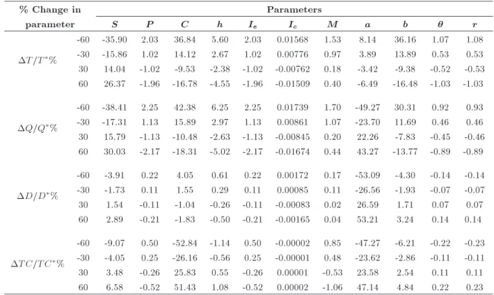
Table 1. Sensitivity analysis.
% Change in Parameters
parameter S P C h Ie Ic M a b r
T=T%
-60 -35.90 2.03 36.84 5.60 2.03 0.01568 1.53 8.14 36.16 1.07 1.08 -30 -15.86 1.02 14.12 2.67 1.02 0.00776 0.97 3.89 13.89 0.53 0.53 30 14.04 -1.02 -9.53 -2.38 -1.02 -0.00762 0.18 -3.42 -9.38 -0.52 -0.53 60 26.37 -1.96 -16.78 -4.55 -1.96 -0.01509 0.40 -6.49 -16.48 -1.03 -1.03
Q=Q%
-60 -38.41 2.25 42.38 6.25 2.25 0.01739 1.70 -49.27 30.31 0.92 0.93 -30 -17.31 1.13 15.89 2.97 1.13 0.00861 1.07 -23.70 11.69 0.46 0.46 30 15.79 -1.13 -10.48 -2.63 -1.13 -0.00845 0.20 22.26 -7.83 -0.45 -0.46 60 30.03 -2.17 -18.31 -5.02 -2.17 -0.01674 0.44 43.27 -13.77 -0.89 -0.89
D=D%
-60 -3.91 0.22 4.05 0.61 0.22 0.00172 0.17 -53.09 -4.30 -0.14 -0.14 -30 -1.73 0.11 1.55 0.29 0.11 0.00085 0.11 -26.56 -1.93 -0.07 -0.07 30 1.54 -0.11 -1.04 -0.26 -0.11 -0.00083 0.02 26.59 1.71 0.07 0.07 60 2.89 -0.21 -1.83 -0.50 -0.21 -0.00165 0.04 53.21 3.24 0.14 0.14
T C=T C%
-60 -9.07 0.50 -52.84 -1.14 0.50 -0.00002 0.85 -47.27 -6.21 -0.22 -0.23 -30 -4.05 0.25 -26.16 -0.56 0.25 -0.00001 0.48 -23.62 -2.86 -0.11 -0.11 30 3.48 -0.26 25.83 0.55 -0.26 0.00001 -0.53 23.58 2.54 0.11 0.11 60 6.58 -0.52 51.43 1.08 -0.52 0.00002 -1.06 47.14 4.84 0.22 0.23 5. Numerical example and sensitivity analysis
To illustrate the proposed method, the following two numerical examples are considered. These examples cover the two cases in the model. The sensitivity analysis of the present model is examined for changes in the parameters. In addition, it should be noted that the time units used for M and T in the model are in `years', whereas the units used in the following examples are `days'. The following examples use the assumptions mentioned in Section 2.
Example 1. Given that S = $80=order, P = $5=unit, C = $2=unit, h = $1=unit/year, Ie =
0:1=year, Ic = 0:1/year, M = 30 days= 30=365 years,
a = 3000 units/year, b = 8100 units/year, = 0:1 and r = 0:1, what will be the optimal results?
Using Eq. (14), we obtain that the value of ! is -1.279. Then, according to Part (b) of Theorem 3, we have T = T
2, Q = Q(T2), D = Q(T2), T C =
T C(T
2). Using corresponding equations and methods,
we obtain that T=30.25 days, Q=278.8, D=3364.3,
and T C=7771.679, respectively.
Example 2. Suppose that S = $70=order, P = $6/unit, C = $2/unit, h = $1/unit/year, Ie =
0:1/year, Ic=0.12/year, M = 30 days = 30=365 years,
a = 5000 units/year, b = 10000 units/year, = 0:1, r = 0:06.
Computing !, the value of ! is 35.619. Then,
according to Part (a) of Theorem 3, we have T= T 1,
Q= Q(T
1), D= Q(T1)=T1, T C= T C(T1). Using
corresponding equations and methods, we obtain that T = 24:58 days, Q = 361:4, D = 5366:2, T C =
11802:199, respectively.
Next, we will study the eects of changes in the values of parameters on the optimal values of T, Q,
D and T C. The sensitivity analysis is examined by
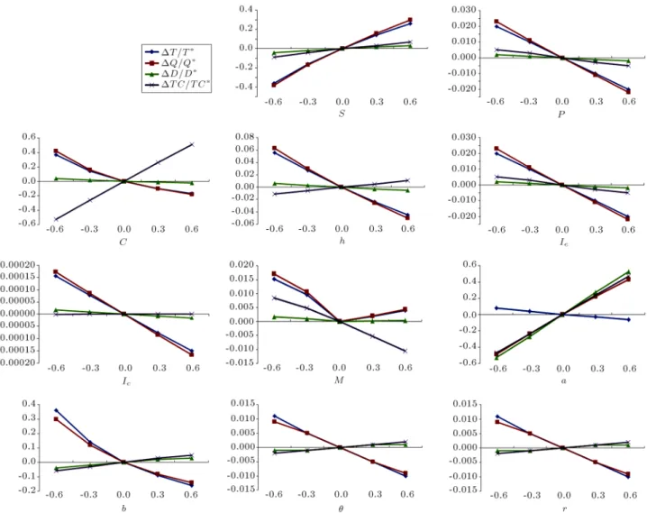
changing the value of each parameter by 60%, 30%, 30% and 60%, taking one parameter at a time and keeping the values of the remaining parameters. The sensitivity analysis is based on the Example 1. and the results are given in Table 1. In addition, in order to better understanding, the sensitivity analysis has been graphed in Figure 1 based on the data in Table 1.
The following points and inferences are obtained:
(i) T, Q, D, and T Cincrease with the increase
in the value of parameter S. A simple econom-ical interpretation is that the retailer will place orders with less frequency to avoid the larger ordering cost. Furthermore, T and Q are
moderately sensitive to the parameter S; T C
is lowly sensitive to the parameter S; and Q is
insensitive to changes in S.
(ii) T, Q, D, and T C decrease as the value
of parameter P or Ie increase. It indicates
that a larger selling price or interest earned rate leads to a higher interest being earned during the trade credit period. Therefore, the retailer
Figure 1. Sensitivity analysis of the parameters for the presented model. places orders with more frequently. However,
T, Q, D and T C are all insensitive to
parameters P and Ie.
(iii) T, Q, and D decrease while T C increase
with the increase in the value of parameter C. It shows that a higher purchasing cost leads to a higher inventory cost and then the retailer will order lower quantity to reduce the higher stock cost. T and Q are moderately sensitive while
T C is highly sensitive to parameter C. D is
insensitive to changes in C.
(iv) T, Q, and D decrease while T C increases
with the increase in the value of parameter h. Its economical interpretation is similar to parameter C. Furthermore, Tand Qare lowly
sensitive while D and T C are insensitive to
parameter h.
(v) T, Q, and D decrease while T C increase
with the value of parameter Ic increasing. In
addition, T, Q, Dand T Care all insensitive
to parameter Ic. Note that Icis most insensitive,
than the other parameters, to the all optimal values.
(vi) T Cdecreases while T, Q, and Ddecrease at
beginning and then increase with the increase in the value of parameter M. However, T, Q, D,
and T C are all insensitive to parameter M. (vii) T is decreasing while Q, D, and T C are
increasing with the increase in the value of parameter a, which is consistent with the eco-nomic sense. In addition, Q, D, and T C are
highly sensitive, while T is lowly sensitive to
parameter a.
(viii) T and Q decrease while Dand T C increase
with the increase in the value of parameter b. Its economical interpretation is similar to parameters P and Ie. T and Q are
moder-ately sensitive while T C is lowly sensitive to
parameter C. Additionally, D is insensitive to
changes in b.
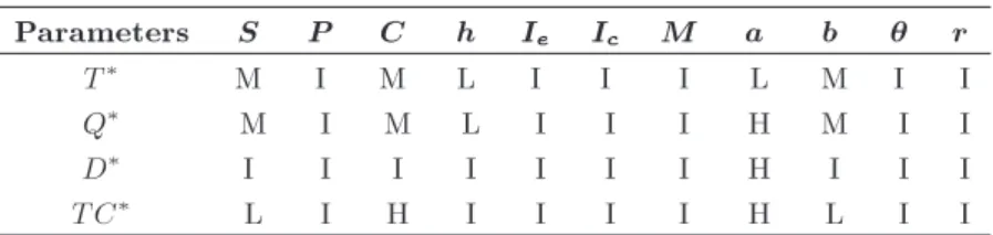
(ix) Tand Q decrease, while Dand T C increase
Table 2. Sensitivity hierarchies.
Parameters S P C h Ie Ic M a b r
T M I M L I I I L M I I
Q M I M L I I I H M I I
D I I I I I I I H I I I
T C L I H I I I I H L I I
H-highly sensitive; M-moderately sensitive; L-lowly sensitive; I-insensitive.
r. Their economical interpretation is similar to parameter C. Nevertheless, T, Q, D, and
T C are all insensitive to parameters and r.
It implies that some errors in estimating or r may result in little deviation from the optimal results.
According to the above analysis and description, we may obtain sensitivity hierarchies between parameters and the optimal values. The results are shown in Table 2.
6. Conclusions
Most of the previous inventory models allowing a permissible delay in payments have usually assumed that the demand is constant or merely dependent on the inventory level or others. In this paper, we develop an inventory model with inventory-dependent and linear trend demand under a permissible delay in payments for deterioration items. The main dierence of this model compared to most existing studies is that we propose a more general inventory model by considering the following aspects: (i) The linear trend demand rate increases signicantly during the growth stage of the product life cycle; (ii) The demand is also linearly dependent on the retailer's instantaneous inventory level; (iii) Deterioration rate is constant; and (iv) The supplier oers the retailer trade credit nancing.
We adopt cost minimization as our objective to determine the optimal order policy. In addition, the conditions of the existence and uniqueness of optimal solution are discussed in detail and an ecient solution is developed to solve the proposed problem. Further-more, we establish Theorem 3 by which we nd a way to obtain the optimal ordering policies by examining the explicit conditions. Whereas Assumption (vii) restricts the application scope of the model to some extent, this assumption is rational in reality. Finally, we provide some numerical examples to illustrate the proposed model and their optimal solutions, and we also obtain some main managerial insights through the sensitivity analysis. Meanwhile, we obtain sensitivity hierarchies between parameters and the optimal values.
When there is no demand stimulation (i.e., =0),
no deterioration rate (i.e., r=0), no increasing demand (i.e., b=0) and no trade credit (i.e., M=0), the pro-posed model may be reduced to the standard EOQ model. Furthermore, as shown in Appendix C, Teng et al. [42] may be viewed as special case.
The present model may be extended in several ways. For instance, we may extend the model to allow for a varying rate of inventory-dependent demand. In addition, we could consider steady decrease demand rate or quadratic time-varying demand rate. Fur-thermore, we could generalize the model to allow for shortages and partial backlogging, partially permissible delay in payments, quantity discounts, relaxation ter-minal condition of zero-ending inventory and ination rates, among others. Therefore, the eects of all of these may be incorporated into future research. Acknowledgments
The authors thank the editor, and the anonymous reviewers for their helpful suggestions. This work is supported by the National Natural Science Foun-dation of China (71471006), Shandong Province Soft Science Research Plan Project (2014RKB01289), Qing-dao City Social Science Planning Research Project (QDSKL140438) and Shandong Province Higher Edu-cational Science and Technology Program (J13WG25). References
1. Goyal, S.K. \Economic order quantity under condi-tions of permissible delay in payments", J. Oper. Res. Soc., 36(4), pp. 335-338 (1985).
2. Goyal, S.K., Teng, J.T. and Chang, C.T. \Optimal ordering policies when the supplier provides a progres-sive interest scheme", Eur. J. Oper. Res., 179(2), pp. 404-413 (2007).
3. Chung, K.J. \A theorem on the determination of eco-nomic order quantity under conditions of permissible delay in payments", Comput. Oper. Res., 25(1), pp. 49-52 (1998).
4. Aggarwal, S.P. and Jaggi, C.K. \Ordering policies of deteriorating items under permissible delay in pay-ments", J. Oper. Res. Soc., 46(5), pp. 658-662 (1995).
5. Jamal, A.M.M. and Sarker, B.R. \An ordering policy for deteriorating items with allowable shortage and
permissible delay in payment", J. Oper. Res. Soc., 48(8), pp. 826-833 (1997).
6. Chang, H.J. and Dye, C.Y. \An inventory model for deteriorating items with partial backlogging and permissible delay in payments", Int. J. Sys. Sci., 32(3), pp. 345-352 (2001).
7. Teng, J.T. \On the economic order quantity under conditions of permissible delay in payments", J. Oper. Res. Soc., 53(8), pp. 915-918 (2002).
8. Mohan, S., Mohan, G. and Chandrasekhar, A. \Multi-item, economic order quantity model with permissible delay in payments and a budget constraint", Eur. J. Ind. Eng., 2(4), pp. 446-460 (2008).
9. Chang, C.T., Ouyang, L.Y. and Teng, J.T. \An EOQ model for deteriorating items under supplier credits linked to ordering quantity", Appl. Math. Model., 27(12), pp. 983-996 (2003).
10. Chung, K.J., Goyal, S.K. and Huang, Y.F. \The optimal inventory policies under permissible delay in payments depending on the ordering quantity", Int. J. Prod. Econ., 95(2), pp. 203-213 (2005).
11. Ouyang, L.Y., Teng, J.T., Goyal, S.K. and Yang, C.T. \An economic order quantity model for deteriorating items with partially permissible delay in payments linked to order quantity", Eur. J. Oper. Res., 194(2), pp. 418-431 (2009).
12. Chen, S.H., Cardenas-Barron L.E. and Teng, J.T. \Retailer's economic order quantity when the supplier oers conditionally permissible delay in payments link to order quantity", Int. J. Prod. Econ., 155(51), pp. 284-291 (2014).
13. Huang, Y.F. \Optimal retailer's ordering policies in the EOQ model under trade credit nancing", J. Oper. Res. Soc., 54(9), pp. 1011-1015 (2003).
14. Teng, J.T. and Goyal, S.K. \Optimal ordering policies for a retailer in a supply chain with up-stream and down-stream trade credits", J. Oper. Res. Soc., 58(9), pp. 1252-1255 (2007).
15. Kreng, B.V. and Tan, S.J. \The optimal replenishment decisions under two levels of trade credit policy de-pending on the order quantity", Exp. Sys. Appl., 37(7), pp. 5514-5522 (2010).
16. Chang, C.T., Teng, J.T. and Goyal, S.K. \Inventory lot-size models under trade credits: A review", A. Pac. J. Oper. Res., 25(1), pp. 89-112 (2008).
17. Chung, K.J. and Cardenas-Barron, L.E. \The simpli-ed solution procsimpli-edure for deteriorating items under stock-dependent demand and two-level trade credit in the supply chain management", Appl. Math. Model., 37(7), pp. 4653-4660 (2013).
18. Ouyang, L.Y., Yang, C.T., Chan, Y.L. and Cardenas-Barron, L.E. \A comprehensive extension of the opti-mal replenishment decisions under two levels of trade credit policy depending on the order quantity", Appl. Math. Comput., 224(1), pp. 268-277 (2013).
19. Yadav, D., Singh, S.R. and Kumari, R. \Retailer's optimal policy under ination in fuzzy environment with trade credit", International Journal of Systems Science, 46(4), pp. 754-762 (2015).
20. Guchhait, P., Maiti, M.K. and Maiti, M. \Two storage inventory model of a deteriorating item with variable demand under partial credit period", Appl. Soft Com-put., 13(1), pp. 428-448 (2013).
21. Chung, K.J., Cardenas-Barron, L.E. and Ting, P.S. \An inventory model with non-instantaneous receipt and exponentially deteriorating items for an integrated three layer supply chain system under two levels of trade credit", International Journal of Production Economics, 155(51), pp. 310-317 (2014).
22. Wu, J., Ouyang, L.Y, Cardenas-Barron, L.E. and Goyal, S.K. \Optimal credit period and lot size for deteriorating items with expiration dates under two-level trade credit nancing", Eur. J. Oper. Res., 237(3), pp. 898-908 (2014).
23. Levin, R.I., Mclaughlin, C.P., Lamone, R.P. and Kot-tas, J.F., Productions/Operations Management: Con-temporary Policy for Managing Operating Systems, p. 373, McGraw-Hill, New York (1972).
24. Gupta, R. and Vrat, P. \Inventory model for stock-dependent consumption rate", Opsear., 23(1), pp. 19-24 (1986).
25. Baker, R.C. and Urban, T.L. \A deterministic inven-tory system with an inveninven-tory-level-dependent demand rate", J. Oper. Res. Soc., 39(9), pp. 823-831 (1988).
26. Su, C.T., Tong, L.I. and Liao, H.C. \An inventory under ination for stock dependent consumption rate and exponential decay", Opsear., 33, pp. 71-88 (1996).
27. Widyadana, G.A., Cardenas-Barron, L.E. and Wee, H.M. \Economic order quantity model for deterio-rating items and planned backorder level", Math. Comput. Model., 54(5-6), pp. 1569-1575 (2011).
28. Cardenas-Barron, L.E. \Optimal ordering policies in response to a discount oer: Extensions", Int. J. Prod. Econ., 122(2), pp. 774-782 (2009).
29. Balakrishnan, A., Pangburn, M.S. and Stavrulaki, E. \Stack them high, let `em y": Lot-sizing policies when inventories stimulate demand", Man. Sci., 50(5), pp. 630-644 (2004).
30. Liao, H.C., Tsai, C.H. and Su, C.T. \An inventory model with deteriorating items under ination when a delay in payments is permissible", Int. J. Prod. Econ., 63(2), pp. 207-214 (2000).
31. Sana, S.S. and Chaudhuri, K.S. \A deterministic EOQ model with delays in payments and price-discount oers", Eur. J. Oper. Res., 184(2), pp. 509-533 (2008).
32. Soni, H. and Shah, N.H. \Optimal ordering policy for stock-dependent demand under progressive payment scheme", Eur. J. Oper. Res., 184(1), pp. 91-100 (2008).
33. Min, J., Zhou, Y.W. and Zhao, J. \An inventory model for deteriorating items under stock-dependent
demand and two-level trade credit", Appl. Math. Model., 34(11), pp. 3273-3285 (2010).
34. Min, J., Zhou, Y.W., Liu, G.Q. and Wang, S.D. \An EPQ model for deteriorating items with inventory-level-dependent demand and permissible delay in pay-ments", Int. J. Sys. Sci., 43(6), pp. 1039-1053 (2012).
35. Sarkar, B. \An EOQ model with delay in payments and time varying deterioration rate", Math. Comput. Model., 55(3), pp. 367-377 (2012).
36. Silver, E.A. and Meal, H.C. \A simple modication of the EOQ for the case of a varying demand rate", Prod. Invent. Man., 10(4), pp. 52-65 (1969).
37. Wee, H.M. \A deterministic lot-size inventory model for deteriorating items with shortages and a declining market", Comput. Oper. Res., 22(3), pp. 345-356 (1995).
38. Omar, M. and Smith, D.K. \An optimal batch size for a production system under linearly increasing time-varying demand process", Comput. Ind. Eng., 42(1), pp. 35-42 (2002).
39. Sarkar, T., Ghosh, S.K. and Chaudhuri, K.S. \An opti-mal inventory replenishment policy for a deteriorating item with time-quadratic demand and time-dependent partial backlogging with shortages in all cycles", Appl. Math. Comput., 218(18), pp. 9147-9155 (2012).
40. Chang, H.J., Hung, C.H. and Dye, C.Y. \An inventory model for deteriorating items with linear trend demand under the condition of permissible delay in payments", Prod. Plan. Control., 12(3), pp. 274-282 (2001).
41. Khanra, S., Ghosh, S.K. and Chaudhuri, K.S. \An EOQ model for a deteriorating item with time de-pendent quadratic demand under permissible delay in payment", Appl. Math. Comput., 218(1), pp. 1-9 (2011).
42. Teng, J.T., Min, J. and Pan, Q.H. \Economic order quantity model with trade credit nancing for non-decreasing demand", OMEGA, 40(3), pp. 328-335 (2012).
43. Dye, C.Y. and Ouyang, L.Y. \An inventory models for perishable items under stock-dependent selling rate and time-dependent partial backlogging", Eur. J. Oper. Res., 163(3), pp. 776-783 (2005).
44. Koschat, M.A. \Store inventory can aect demand: Empirical evidence from magazine retailing", J. Re-tail., 84(2), pp. 165-179 (2008).
45. Dave, U. and Patel, L.K. \(T, Si) policy inventory model for deteriorating items with time proportional demand", J. Oper. Res. Soc., 32(2), pp. 137-142 (1981).
46. Chung, K.J. \Viewpoints: An EOQ model for deteri-orating items under trade credits by Ouyang, Chang and Teng", J. Oper. Res. Soc., 59(10), pp. 1425-1430 (2008).
Appendix A Proof of lim
T !1k2(T ) = +1.
k2(T ) = S + h
Z T
0
(aT + bT2)e(+r)(T t)
I(t)
dt + CIc
Z T
M
(aT + bT2)e(+r)(T t)
I(t)
dt + C
(aT + bT2)e(+r)T Q
P Ie
Z M
0 (aT + bT
2)(M t)e(+r)(T t)dt
Z M
0 (a + bt + I(t))(M t)dt
:
By using L'Hospital rule and assumption (vii), it is easy to obtain Eqs. (A.1) to (A.3) as shown in Box II. From the analysis conducted so far, we can conclude that lim
T !+1k2(T ) = +1.
Appendix B
If !>0, according to Theorem 1, we obtain T C1(T1) >
T C1(M). In addition, using T C1(M) = T C2(M), and
Theorem 2, we have T C1(T1) > T C1(M) = T C2(M) >
T C2(T ) for all T > M. It thus proves Part (a) of
Theorem 3. Likewise, Parts (b) and (c) of Theorem 3 may be proved in a similar manner.
Appendix C
Special case of the presented model. When ! 0+, r ! 0+, the proposed model may be reduced to
the model of Teng et al. [42]. By using L'Hospital rule, from Eqs. (3), (4), (5) and (6), we obtain:
I(t) = lim
!0+r!0lim+
[( + r)(a + bT ) b] e(+r)(T t)
( + r)(a + bt) + b
=( + r)2= a(T t)
+12b(T2 t2); 0 t T; (C.1)
Q = I(0) = lim
!0+r!0lim++
[( + r)(a + bT ) b]
e(+r)T ( + r)a + b=( + r)2=aT +1
2bT(C.2)2;
T C3(T ) = lim
!0+r!0lim+T C1(T ) = lim!0+r!0lim+
1 T
S
lim
T !+1
(aT + bT2)RT
0 e(+r)(T t)dt
RT 0 I(t)dt
= lim
T !+1
(a + 2bT )R0Te(+r)(T t)dt + (aT + bT2) + ( + r)(aT + bT2)RT
0 e(+r)(T t)dt
(a + bT )R0Te(+r)(T t)dt
> lim
T !+11 + ( + r)T = +1 (A.1)
lim
T !+1
C(aT + bT2)e(+r)T Q
P Ie
h
R0M(aT + bT2)(M t)e(+r)(T t)dt RM
0 (a + bt + I(t))(M t)dt
i
= lim
T !+1
C( + r)2
P Ie( + r)M + e (+r)M 1 1; (A.2)
lim
T !+1
RT
M(aT + bTR 2)e(+r)(T t)dt T
MI(t)dt
= lim
T !+1
RT
M(a + 2bT )e(+r)(T t)dt + (aT + bT2) + ( + r)(aT + bT2)
RT
Me(+r)(T t)dt
RT
M(a + bT )e(+r)(T t)dt
> lim
T !+11 + ( + r)T = +1: (A.3)
Box II
+h
a + bT ( + r)2
b
( + r)3(e(+r)T 1)
2aT + bT2
2( + r) + bT ( + r)2
+C[( + r)(a + bT ) b] e( + r)(+r)T2 ( + r)a + b
P Ie
r 6aT M + 3bMT2 3aT2 2bT3 6( + r)
+( + r)(a + bT ) b( + r)2
T M + Me(+r)T
+ r +1 e( + r)(+r)T2
+b(2MT2( + r)2T2)
= 1 T
S + (h + P Ie)
1 2aT2+
1 3bT3
+(C P MIe)
aT +12bT2; if T M;
(C.3) T C4(T ) = lim
!0+r!0lim+T C2(T ) = lim!0+r!0lim+
1 T
S
+h
a + bT ( + r)2
b
( + r)3(e(+r)T 1)
2aT + bT2
2( + r) + bT ( + r)2
+C[( + r)(a + bT ) b] e(+r)T ( + r)a + b ( + r)2
+CIe
(a + bT )( + r)2 b
(e(+r)(T M) 1)
( + r)3
2aT + bT2 2aM bM2
2( + r) +
b(T M) ( + r)2
P Ie
r(3aM2+ bM3)
6( + r) +
( + r)(a + bT ) b ( + r)2
Me(+r)T
+ r +
e(+r)(T M) e(+r)T
( + r)2
+2( + r)bM22
= T1
1 2aT2+
1 3bT3
+ (C CMIc)(aT +12bT2)
+(CIc P Ie)(12aM2+16bM3)
if T M: (C.4) Then, Eqs. (7) may be reduced as follows:
T C(T ) = 8 < :
T C3(T ) T M
T C4(T ) T M
(C.5)
Eqs. (C.5) are consistent with Eqs. (6) and (7), respec-tively, in Teng et al.'s model [42]. Therefore, the model of Teng et al. is a special case of this paper. Note that Teng et al.'s model is a prot function.
Biographies
Chengfeng Wu is a full-time instructor in the De-partment of Logistics at Qingdao University of Science
and Technology. He received his PhD degree in the Department of Management Science at Beihang University, P.R. China. His research interests include inventory control, supply chain management, etc. His articles have appeared in journals such as Interna-tional Transactions in OperaInterna-tional Research and In-ternational Journal of Systems Science: Operations & Logistics.
Qiuhong Zhao is a Professor of Management Science at Beihang University, P.R. China. She received her PhD degree in Management Science from Beihang Uni-versity. Her major research elds include production and operation management, supply chain and logistics management, emergency management, meta-heuristics algorithms, etc. Her articles have appeared in journals such as Computers and Operations Research, Euro-pean Journal of Operational Research, Computers and Industrial Engineering, Omega-International Journal of Management Science, Applied Mathematics and Computation, Engineering Optimization.