2. Escobedo, J. and Mansoori, G.A. \Solid particle depo-sition during turbulent ow production operations", SPE paper #29488, Proceed. Soc. Petrol Eng. Produc-tion OperaProduc-tion Symp. Held in Oklahoma City, OK (2-4 Apr. 1995).
3. Branco, V.A.M., Mansoori, G.A., De Almeida Xavier, L.C., Park, S.J. and Mana, H. \Asphaltene occula-tion and collapse from petroleum uids", J. Petrol Sci. & Eng., 32, pp. 217-230 (2001).
4. Mousavi-Dehghani, S.A., Riazi, M.R., Vafaie-Sefti, M. and Mansoori, G.A. \An analysis of methods for deter-mination of onsets of asphaltene phase separations", J. Petrol Sci. & Eng., 42(2-4), pp. 145-156 (2004). 5. Mansoori, G.A., Vazquez, D. and Shariaty-Niassar,
M. \Polydispersity of heavy organics in crude oils and their role in oil well fouling", J. Petrol. Sci. and Engineering, 58(3-4), pp. 375-390 (2007).
6. Lichaa, P.M. and Herrera, L. \Electrical and other eects related to the formation and prevention of asphaltene deposition in Venezuela", Paper SPE paper #5304, Proceed. Soc. of Petrol Eng. Intl. Symposium on Oileld Chemistry, Dallas TX (Jan. 16-17, 1975). 7. Ray, R.B., Witherspoon, P.A. and Grim, R.E. \A
study of the colloidal characteristic of petroleum using the ultracentrifuge", J. Phys. Chem., 61, pp. 1296-1302 (1957).
8. Katz, D.H. and Beu, K.E. \Nature of asphaltic sub-stances", Ind. Eng. Chem., 37, pp. 195-200 (1945). 9. Eliassi, A., Modaress, H. and Mansoori, G.A. \Study
of asphaltene occulation using particle counting method", Proceed. Filtech 2005 (Int.'l Conf. & Exhib for Filteration & Separation Tech), I, pp. 506-511, Weisbaden, Germany (11-13 Oct. 2005).
10. Lin, C.S., Moulton, R.W. and Putnam, G.L. \Mass transfer between solid wall and uid streams", Ind. Eng. Chem., 45, pp. 636-646 (1953).
11. Lauufer, J. \The Structure of turbulence in fully developed pipe ow", NACA 1174, National Advisory Committee for Aeronautics (Available from NASA as TR-1174) (1954).
12. Friedlander, S.K. and Johnstone, H.F. \Deposition of suspended particles from turbulent gas streams", Ind. Eng. Chem., 49(7), pp. 1151-1156 (July 1957). 13. Beal, S.K. \Deposition of particles in turbulent ow on
channel or pipe walls", Nuclear Sci. Eng., 40, pp. 1-11 (1970).
14. Derevich, I.V. and Zaichik, L.I. \Particle deposition from a turbulent ow", Fluid Dynamics, 23(5), pp. 722-729 (1988).
15. Tandon, P. and Adewumi, M.A. \Particle deposition from turbulent ow in a pipe", J. Aerosol. Sci., 29(1-2) pp. 141-156 (1998).
16. Harriott, P. and Hamilton, R.M. \Solid-liquid transfer in turbulent pipe ow", Chem. Eng. Sci., 20, pp. 1073-1078 (1965).
17. Shapiro, M., Brenner, H. and Guell, D.C. \Accumu-lation and transport of Brownian particles at solid surfaces: Aerosol and hydrosol deposition processes", J. Colloid Inter. Sci., 136(2), pp. 552-558 (1990). 18. Johansen, S.T. \The deposition of particles on vertical
walls", Int. J. Multiphase Flow, 17(3), pp. 355-362 (1991).
19. Von Karman, T., Aerodynamics: Selected Top-ics in the Light of Their Historical Development, www.doverpublications.com (2004).
20. Mansoori, G.A. \ASPHRAC: A comprehensive package of computer programs and database which calculates various properties of petroleum uids containing heavy organics", www.uic.edu/ mansoori/ASPHRAC html
Invited Paper
Predicting Corrosion in Pipelines, Oil Wells and
Gas Wells; a Computer Modeling Approach
F.F. Farshad
1;, J.D. Garber
2, H.H. Rieke
3and Sh.G. Komaravelly
2Abstract. Hostile oileld corrosive environments have challenged the production and transportation operations of the petroleum industry. The estimated cost of corrosion on the U.S. economy in the year 2002 resulted in an expenditure of about 276 billion U.S. dollars. This amount was an increase of more than $100 billion over a previous ve year period. Corrosion maintenance expenditures over this 5 year period were approximately 3.1% of the U.S. GDP, and stimulated congress to enact the Corrosion Prevention Act in 2007. One avenue available to successfully combat corrosion in the petroleum industry is the recent progress made in corrosion prediction applications for petroleum operations. Three such corrosion computer models have been developed at the University of Louisiana at Lafayette. These models are capable of predicting the physical conditions and corrosion rates inside pipelines and in producing oil and gas wells. The models are window based and described in this paper. An expert system module was developed, which adjusts the predicated corrosion rate based on various known reservoir and well subsurface parameters. Keywords: Pipeline corrosion modeling; Oil and gas corrosion modeling; Flow assurance.
INTRODUCTION
Corrosion can be dened as the destruction of a metal by chemical or electrochemical reactions, or microbial reaction with its environment. The principles of corrosion must be established in order to eectively select materials, and provide the design and fabrication of Oil Country Tubular Goods (OCTG) and production facilities in such a manner as to optimize their eco-nomic life and ensure safety in petroleum operations. Mitigation of corrosion is an important integral part of combating ow assurance problems [1]. Until recently, no single text book devoted to petroleum science and engineering aspects of corrosion was available until one was authored by Chilingar [2].
1. College of Engineering, Department of Chemical Engineer-ing, University of Louisiana at Lafayette, P.O. Box 40083, Lafayette, LA 70504, USA.
2. College of Engineering, Department of Chemical Engineer-ing, University of Louisiana at Lafayette, P.O. Box 44130, Lafayette, LA 70504-4130, USA.
3. College of Engineering, Department of Petroleum Engineer-ing, University of Louisiana at Lafayette, P.O. Box 44690, Lafayette, LA 70504-4690, USA.
*. Corresponding author. E-mail: farshaddr@gmail.com Received 11 July 2009; received in revised form 8 January 2010; accepted 1 February 2010
The basic fundamentals of corrosion are the same for all metals and alloys, and dier in degree and not in kind [3]. The factors which inuence corrosion are divided into two groups. Group one delineates factors associated mainly with metals. These include:
Eective electrode potential of the metal. Overvoltage of hydrogen on the metal.
Tendency of metal to form an insoluble protective lm.
Chemical and physical homogeneity of metal sur-face.
Nature, concentration and distribution of elec-trolytes.
Environmental tendency to deposit a protective lm on the metal surface.
Solution ow rate against metal.
Environmental temperature and pressure. Static or cyclic stresses.
Contact with dissimilar solutions. Contact with dissimilar metals.
Microbial activity that forms H2S, sulfur bearing
During well drilling, general corrosion control practices in petroleum operations involve the use of a high pH mud containing a corrosive inhibitor. The well completion practice uses a cement sheath and bond between the pipe and the formation to protect the casing by controlling water inow into the well. The pipe mill scale is controlled by pickling (5-10% H2SO4 or 5% HCl at 180F with inhibitors) or by
sand blasting [2]. Bactericides or oxygen scavengers are used to control corrosion in the subsurface. Cathodic protection is not a practical method for controlling corrosion of drill pipes or the internal surface of the well casing. Chilingar [2] pointed out that cathodic production is best used in the protection of pipelines and owlines.
Today, newly developed computer models help combat corrosion and predict corrosion rates for a variety of petroleum production operations. Such computer models were developed at the University of Louisiana at Lafayette, Corrosion Research Center. The models are capable of predicting corrosion rates in oil wells, gas wells and pipelines. Development of the models was sponsored by industry and the United States Department Of Energy (DOE) [4]. The oil and gas modeling results provide a physical description of what is happing inside production wells, as a function of well depth [5,6]. An overview of the computer models is presented to demonstrate the technical advances in corrosion mitigation in vertical production hydrocar-bon wells, pipelines and owlines.
PIPELINE MODEL
A new pipeline model has been developed that can predict the corrosion rate in gas and oil owlines and pipelines. The program describes the physical and chemical conditions inside a pipeline. This model predicts the corrosion rate in systems containing CO2,
H2S, organic acid and bacteria. The above model
predicts the occurrence of \top of the line" corrosion, internal wettability conditions and describes ow dy-namics in large diameter pipelines. Furthermore, the model is capable of providing risk assessment which allows for integrity management of the system [7]. Physical Description
The rst three modules shown in Figure 1 give the owchart description of a process modeling. This includes a temperature/pressure prole, the phases present and the ow dynamics at each point in the pipe. In the case of CO2 corrosion, the ow regime
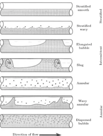
is very critical to the prediction of the corrosion rate. Typical horizontal ow regimes are described by the model in Figure 2. The ow dynamic model includes empirical corrosion rate prediction.
Figure 1. The three models that are looped for pressure convergence.
Figure 2. Flow pattern for horizontal two-phase ow.
Chemical Prole
The model is capable of predicting the chemical prop-erties of the water in the system. In a system containing condensed water, the pH is low and so is the ion concentration. It is possible to track the location of organic acids entering the system, as well as bicarbonates and other ions. The potential for scale can be predicted by this model.
Corrosion Rate Prole
The nal and most dicult part of the model is determination of the corrosion rate. Using equations developed in our previous models, we obtained accurate estimates of the corrosion rate at each point in the
pipeline system. In addition to the more empirical models, a pitting corrosion model has also been in-cluded, which estimates the theoretical pitting rate. This model requires that a water analysis be available. To provide the best estimate of the actual corro-sion rate, an expert system has been developed. The parameters that are considered are temperature, water wetting, % inhibition, scaling and microbial eect. Risk Assessment
Risk Assessment is useful in evaluating the life of various systems. General corrosion models predict the corrosion rate on a deterministic basis, namely all the input values are known and are xed. However, in reality, each input will have some uncertainty asso-ciated with it because of the variation of production conditions and environment. This variation can have a signicant impact on the corrosion rate prediction. One way to solve this problem is to calculate the range of corrosion rates based on the whole range of input values. This process can be time consuming if many inputs are involved.
Pitting Corrosion
There are, in total, 20 parameters used as inputs to de-termine corrosion rate in the pitting model. Variations of some of the 20 parameters have a signicant impact on the predicted corrosion rate, and others have only a minor impact. Attaching a random number generator to all these variables will be time consuming and unnec-essary. In this work, major variables are distinguished from minor variables in terms of their inuence on the corrosion rate, and only major variables are considered to be associated with certain distribution types. The minor variables will be evaluated on their input basis. Specifying the typical range of each variable in the eld, the corrosion rate is calculated by continu-ously changing one variable in the range with others xed. The resulting maximum and minimum corrosion rates are compared, giving the percent change of the corrosion rate for that particular variable. The eect of each variable on the corrosion rate was determined and it can be seen by our data that bicarbonate, temperature, CO2 mole fraction, pipe wall thickness,
chlorides, pressure and bulk iron have an eect on the corrosion rate in the range assigned [7].
MAJOR VARIABLES
In this work, eld data and assumptions from the literature are combined to determine the distribution type of major variables. Based on 11,838 water analyses from oil and gas companies, distributions have been found for the following variables:
Alkalinity (bicarbonate): log-normal. pH: normal.
Chlorides: log-normal or normal.
A corrosion rate distribution of 20,000 iterations with assigned distribution type inputs resulted in a calcu-lated mean corrosion rate of 20.7 mpy, and the standard deviation equals 9.54 mpy. The actual predicted corrosion rate was calculated to be 19.6 mpy by using the mean value for normal and log-normal type inputs and the average value between the lower and upper limit for uniform type inputs.
This ratio is the same as quoted by investigators of the Norsok and DeWaard Milliams [7] models for local corrosion. This result is encouraging, because it validates the random number generators and also the pitting model. In the model, due to time con-straints, the standard deviation was xed at 45% of the predicted corrosion rate, even though it will normally range from 35% to 55%, depending on input values.
CLASSIFICATION OF RISK ASSESSMENT With the knowledge of probability of failure, the risk category of the pipe can be identied based on the criteria proposed in the DNV RP-G101 stan-dard [7].
OIL WELL MODEL
An oil well computer model is developed that is capable of predicting physical conditions and corrosion rates inside a vertical or deviated well at various depths and under naturally owing or gas lift conditions [4]. The model contains ve specic parts. The following describes the ve main parts of the model.
1. Temperature/Pressure Prole: This program calculates the temperature and pressure prole at various depths in an oil well. The model uses the method of Articial Neural Networks (ANN) to establish the temperature prole. Farshad et al. [8] developed a neural network based methodology to predict the uid temperature prole in producing multiphase oil wells. The initial values used in the pressure calculation assume a linear pressure prole between the wellhead and bottomhole pressure values. A looping routine was used to estimate the pressure drop in an oil well.
2. Phase Behavior Prole: Prediction of the hy-drocarbon phases that are at equilibrium at various depths in the well was undertaken using the Peng-Robinson equation of state. This model rst matches the ow rates of the gas-oil-water phases in the separator using gas composition, gravity of
oil, temperature and pressure. Once the ow rates in the separator are matched by looping, the overall composition of the full production stream can then be determined. The program then performs the phase equilibrium calculation to bottomhole. 3. Flow Dynamics Prole: Once the phase
equi-librium information is known, it is possible to establish the ow dynamics at various depths in a [9] well. Figure 2 was used to provide the best overall description of the transition points between bubble, slug and churn ow regimes in an oil well. The three ow regimes are shown in Figure 3 for a non-annular owing oil well. The liquid and gas [9] supercial velocities calculated in Figure 2 can be used to identify which regime occurs at any location in an oil well.
The equations described by Fernandes [10] are the ones being used to physically describe the slug unit, as shown in Figure 4. One of the parameters that come from this calculation is the length of the liquid slug. Calculations have shown, in over 50 wells tested, that the void fraction at the point when the length of the Taylor bubble became negative was approximately 0.275. This value was, therefore, adopted as the point of slug to bubble transition.
4. Corrosion Rate Prole: Garber et al. [4] pointed out that the primary objective of this model was to use the physical parameters generated at each point in the production tubing to develop an empirical correlation with the corrosion rate. Inasmuch as oil inhibition is a problem in the prediction of the corrosion rate in oil wells, uid data from non-annular gas condensate wells was used in the correlation. Four parameters, plus this one, were established to produce an empirical corrosion rate model for vertical owing oil wells.
Figure 3. Flow pattern for vertical two-phase ow.
Figure 4. Slug unit in an oil well.
5. Corrosion Rate Expert System Component: Factors to be considered in developing a corrosion rate expert system for oil wells are:
Water wetting eect. Eect of ow regime. Temperature eect. Inhibitive eect.
These factors have been shown to be important by various investigators who have worked in the area of CO2 corrosion for many years. The factors are used
to adjust the predication rate for an oil well. GAS WELL MODEL
A gas well computer model was developed [6], which can help predict the location of corrosion and the life of carbon steel tubular in a gas condensate well containing carbon dioxide. This model provides a physical description for the ve dierent ow regimes that can occur in gas wells. This description has proven to be useful in the prediction of the corrosion rates of these wells. The model does not use the partial pressure of CO2 in calculation of the corrosion rate. It has
been found that the hydrodynamics and the amount of water present are the most important parameters in this type of corrosion. The model has an expert
system associated with it, which takes into account the volume fraction of condensate and water in the tubing. When the water level reaches and exceeds 50% of the total volume, the tubing is completely water-wet and the corrosion rate is a maximum. At the point where 30% or less of the volume of the uid is water, the corrosion rate is believed to be zero. Caliper surveys have played a role in our ability to establish these points of transition within the model. Farshad et al. [6] presented case histories that illustrate how the model can help in performing corrosion failure analysis and in the design of gas condensate wells.
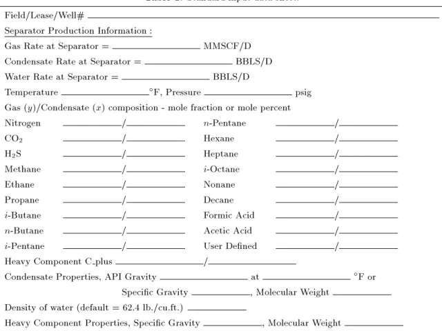
The model provides a physical description of what is happening inside the production tubing as a function of well depth. This type of description has been found to be essential for an accurate prediction of corrosion rates in gas wells. Table 1 is a data sheet that presents the technical input into the model. Five categories of minimum requirements for data input are mandatory to successfully run the model. The minimum required data are:
Completion information, such as true vertical depth, measured depth, size of tubing and casing data, is required.
Temperature and pressure information at the sepa-rator wellhead and bottomhole is required.
Separator production rates of the gas, condensate and oil are required.
Analysis of the gas phase and gravity of the conden-sate are a minimum requirement for the input. A water analysis is needed if the in situ pH is to
be calculated. The model corrects the pH for the presence of organic acid.
The required data, when used, is for a particular time period in the life of the gas wells. Producing gas wells can have compositions and ow rates that normally change with time. This requires multiple modeling of a gas well during its productive life to obtain the necessary picture for corrosion control. The model consists of ve computer modules A, C, E, F and G.
Computer module A calculates the temperature and pressure proles in a well based on computer module G, which produces the bottomhole owing temperature for a given pressure drop as the gas exits through the casing perforations into the well. The phase behavior program which calculates the phases that exists at any point in the tubing is calculated by computer module C. Information from computer module C can help in deciding if the gas well tubing is oil wet or water wet. Computer module E is the ow dynamic model that describes the type of ow regimes present inside the well's tubing, and module F is the model for corrosion rate prediction.
COMPUTER MODULES' PHYSICAL DESCRIPTION
Physical Description Models Models A and G
The rst calculation made with the input data focuses on the temperature and pressure at each depth. Well conguration, number and length of casing and the casing lls constitute the information necessary to calculate the overall heat transfer coecient vs. depth. If the geothermal gradient is known, the heat transfer rate can be determined. The uids inside the well are owing nonisothermally and a microscopic momentum and energy balance calculation on the owing gas produces the equations necessary to calculate both the temperature and pressure drop. Physical properties of the gas and liquids produced inside the tubing are permanently stored in the program for use when needed.
The gas undergoes a substantial pressure drop through the perforations during production. It is possible to estimate the bottomhole owing temper-ature using Model G. This model accounts for the adiabatic expansion of the gas using the Peng-Robinson equation of state. For a typical pressure drop, the temperature of the gas can drop as much as 25F from
its reservoir temperature value. Neglecting this factor can signicantly aect the temperature prole and dew point location.
Model C
Since a gas condensate well is being modeled, one may expect that in addition to gas, both condensate and water could be present inside the tubing. Using the separator production rates and the gas composition, it is possible for the Peng-Robinson EOS to predict the phases present at every depth. If a well is producing formation water, it can be said with certainty that the tubing contains water from the bottomhole to the wellhead. Otherwise, the water may show a dew point somewhere up the tubing. The program can predict this water dew point location. Likewise, the location of condensate inside the tubing is equally important and the model can predict the location of the condensate as well. Therefore, unlike oil wells which produce oil from bottomhole to wellhead, condensate wells may or may not have condensate inside the tubing. Previous work at the center [11] showed that approximately 55% of condensate wells had no condensate inside the tubing, even though there was a substantial amount of condensate in the separator.
Model E
Once it has been established that there is liquid inside the production tubing, it is important to know what type of ow pattern exists at each depth. Figure 3
Table 1. Standard input data sheet. Field/Lease/Well#
Separator Production Information :
Gas Rate at Separator = MMSCF/D
Condensate Rate at Separator = BBLS/D
Water Rate at Separator = BBLS/D
Temperature F, Pressure psig
Gas (y)/Condensate (x) composition - mole fraction or mole percent
Nitrogen / n-Pentane /
CO2 / Hexane /
H2S / Heptane /
Methane / i-Octane /
Ethane / Nonane /
Propane / Decane /
i-Butane / Formic Acid /
n-Butane / Acetic Acid /
i-Pentane / User Dened /
Heavy Component C plus /
Condensate Properties, API Gravity at F or
Specic Gravity , Molecular Weight Density of water (default = 62.4 lb./cu.ft.)
Heavy Component Properties, Specic Gravity , Molecular Weight
Well Information:
Type of Well: On-shore O-shore
Depth of Well to mid-perfs : True Vertical Depth ft, Measured Depth ft
Oshore Well Only:
Depth of Water ft
Sea Level to Wellhead - Length of wellbore exposed to air ft
Temperature of Air F
Wellhead Temperature (owing) F, Pressure (owing) psig
Bottomhole Temperature (static) F, Pressure (static) psig
Production Tubing inside Diameter (ID) inches, Thickness inches
Coated Tubing Yes No
Casing Size inches, Length ft, Annulus Fill
Casing Size inches, Length ft, Annulus Fill
Casing Size inches, Length ft, Annulus Fill
Casing Size inches, Length ft, Annulus Fill
Casing Size inches, Length ft, Annulus Fill
Water Analysis (Optional) Ion Concentration (mg/l)
shows the ve types of ow pattern that can exist in vertical ow. Sixty percent of gas wells studied using Model E were found to be in annular ow at all points in the tubing. Of the remaining wells, 20% were found to be in mist ow at various points in the tubing and 20% were in churn-, slug- or bubble-type ow. A description of how the various ow regimes are modeled follows.
Annular Flow
This type of ow is dened as having the bulk of the liquid owing upward against the pipe wall as a lm. The gas phase is owing in the center of the pipe with some entrained liquid droplets in the gas phase. As described earlier [12], to obtain the liquid lm thickness, it is necessary to calculate the entrained liquid. Then, using a microscopic momentum balance on an element in gas-liquid two-phase ow, it is possible to develop a triangular relationship between pressure gradient, ow rate of liquid lm and liquid lm thickness [12].
Mist Flow
In high velocity wells, the corrosion rate can become activation controlled due to a disturbance of the liquid lm. This has been found to occur whenever (1) the annular ow program calculates that the liquid lm is more than 50% turbulent, or (2) when the liquid droplets become large enough and of sucient velocity to disturb the liquid lm. A paper by Kocamustafaogullari et al. [13] gives an equation for the maximum stable droplet size, in terms of dimensional groups, such as liquid-and gas-phase Reynolds number, modied Weber number and dimensionless physical property groups. Using this concept, a paper [14] on the generation of droplets has shown that for gas condensate wells, the droplets are about 12 times larger in diameter than the thickness of the liquid lm. Their velocities are somewhat less than that of the gas, but it is clear that these are high energy projectiles than can impact the liquid lm causing it to become increasingly turbulent.
The ability to identify mist ow wells based on their abnormally high corrosion rates has been made possible, using a discriminate analysis method [15]. A probability equation has been developed which uses four parameters:
1. Mixture supercial velocity. 2. Reynolds number of liquid.
3. Percent of liquid lm in turbulent ow. 4. Liquid pressure drop.
Based on this relationship, at every depth in an annular ow well, the equation is checked to determine if mist ow exists.
Slug/Churn/Bubble
The remaining 20% of gas wells exist in a ow pattern described as churn, slug or bubble. The approach used in this work was based on considering the slug unit as consisting of one Taylor bubble, its surrounding liquid lm and a liquid pad between the bubbles. Several important parameters, such as the length of the Taylor bubble and the average void fraction of the Taylor bubble and the slug unit were all calculated to within 5 to 10% of the measured values. The void fraction of the slug unit is equivalent to the liquid holdup at each point in the tubing.
This model has also proven to be useful in den-ing the slug/ churn transition point. Mashima and Ishii [16] postulated that direct geometrical parame-ters, such as the void fraction are conceptually simpler and yet more reliable parameters to be used in ow regime criteria than the traditional parameters such as gas and liquid supercial velocities. With this in mind, other work [17] has shown that the vast majority of void fractions for churn ow had a slug unit void fraction of greater than 0.73. None of the reported values below 0.73 were in churn ow [18]. This parameter and its value of 0.73 were selected in this work as the basis of the slug/churn transition point.
Corrosion Rate Model
Since a physical description of each ow regime has been developed, attempts have been made to use these ow parameters to predict corrosion rates in these wells. The following corrosion rate models have been developed.
Annular Flow
As described previously, a well that is in the annular ow regime is usually found to exhibit a liquid lm of a given thickness that can be divided into laminar, buer and turbulent components. Table 2 shows the results of modeling 12 gas wells [12] that had known corrosion rates. The three wells with the thickest lm failed in the shortest period of time. From these data, an excellent tubing life correlation [12,19] based on the rst principle, known as Model F, was developed, which uses the lm thickness and liquid velocity.
Mist Flow
If a well is found to be in mist ow by the pre-viously mentioned discriminate analysis equation, a fundamental change is made to the above corrosion rate correlation. The velocity of the droplet is used in place of the liquid velocity. In most cases, the droplet velocity is within 90% of the gas velocity value. This approach is theoretically more sensible, because it is believed by some investigators that the corrosion rate in mist ow is controlled by droplet impingement [20]. The corrosion under this condition is believed to be
Table 2. Calculated lm thickness in a gas condensate well.
Actual Life Entrainment Calculated Film Thickness (mils)
Well No. (months) % Laminar Buer Turbulent Total
1 44 0.21 1.0 5.0 0.4 6.5
2 117 1.04 0.5 1.6 . . . 2.1
3 113 0.28 1.2 3.5 . . . 4.7
4 59 0.60 0.5 2.4 . . . 3.0
5 71 0.25 1.0 4.5 . . . 5.5
6 116 0.62 0.8 2.9 . . . 3.6
7 62 0.49 1.0 4.4 . . . 5.4
8 91 0.63 1.5 4.2 . . . 5.7
9 97 0.26 1.3 4.1 . . . 5.5
10 32 0.27 1.2 6.1 3.8 11.1
11 41 0.33 0.8 3.8 2.1 6.7
12 66 0.14 1.1 5.0 . . . 6.2
partially activation and mass transfer controlled. In other words, a protective iron carbonates lm forms, which is then physically removed by impingement or by dissolution.
The accuracy of the two above-mentioned corro-sion rate correlations can be seen in Figure 5. The time to failure of 53 gas condensate wells that were in annular or mist ow has been shown to correlate well with the eld data [21]. The average percent dierence between predicted and actual corrosion rates was 18%.
Slug Flow
What has made this model comprehensive is inclusion of the physical description and corrosion prediction for the nonannular ow regime. At this time, a total of only eight gas condensate wells in slug ow with known production and corrosion rates have been documented.
Figure 5. USL model results compared to actual corrosion.
All eight wells contained CO2 as the corrosion specie,
and failed due to internal penetration. The wells were found to be in slug ow at the depth of the failure.
Corrosion rates in slug ow have been experimen-tally determined in the laboratory [22] to be higher than churn ow.
It was decided to develop a correlation for slug ow wells by performing a regression on several of the calculated parameters [5]. The four parameters selected were (1) length of the Taylor bubble, (2) velocity of the Taylor bubble, (3) water rate, and (4) gas supercial velocity. The resulting equation showed an average percent dierence of 14% from the actual value.
To this date, no eld data have been found for the corrosion rate of churn ow wells. It is proposed that the same slug ow regression equation be used and that an experimental factor be applied. The corrosion rate for churn ow gas wells has been found experimentally to be consistently 15% less than slug ow on the experiments conducted [22]. Therefore, at the present time for churn ow wells, the slug parameters are calculated and a 15% reduction factor is applied to the slug corrosion rate equation.
CONCLUSIONS Pipeline Model
The pipeline computer model contains a physical de-scription of large diameter pipes with the modication of the Dukler ow regime maps [23]. Within the ow regime area, the modeling of slug ow has been
the most dicult ow regime to describe. A change in the calculation of the height of the liquid lm has given reasonable slug lengths and liquid hold up values.
The accurate prediction of the wettability of a three-phase of gas-oil-water is important for the deter-mination of the nal corrosion rate. Describing \top of the line" corrosion in a condensing pipeline requires an accurate calculation of the physical system, as well as an accurate knowledge of the ow regime involved. The model is capable of determining if the \top of the line" corrosion can occur and what the pH value is at the top and bottom of the line. By incorporating the eect of organic acid in the calculations, it is possible to predict how seriously it would aect the pipe.
Experimental data has veried that, initially, the CO2 will dominate the corrosion process and a
small amount of H2S will contribute to an increase
in corrosion. However, when the H2S species become
dominant, then, there is usually a drop in the corro-sion rate. Using the pitting model developed at UL Lafayette, it has been possible to model the eect of H2S on CO2 corrosion.
The pipeline model includes an internal risk as-sessment module. The risk asas-sessment module is used to calculate the probability of failure (pof) and provide a risk classication using a 1-5 rating (with 1 the best) as a function of years of use. From this information, a plot of risk classication versus years, to determine the expected time of failure, can be developed. The eect of inhibitors on this classication can also be described. This pipeline program is the \state-of-art" computer model for predicting corrosion in pipelines and owlines with the capability of risk assessment. This program has achieved accurate corrosion rate predictions.
Oil Well Model
An updated computer model was developed that phys-ically describes owing or gas lifted vertical or deviated wells. The model is capable of predicting temperature, pressure, phase behavior and ow dynamics at each depth inside a owing well. The ow regime has a pronounced aect on the pressure drop and corrosion rate inside a well. It was found that the physical description of the Taylor Bubble gave the best indi-cation of when the transition from slug to bubble ow occurred.
Corrosion rates in gas condensate wells correlated well to ve physical parameters for vertical wells. These wells are believed to represent a higher corrosion rate than oil wells due to the inhibitive eect of the crude. The expert system developed for oil wells uses the factors of water cut, ow regime, temperature
and inhibitive eect to adjust the predicted corrosion rate.
The model was tested on several wells in the eld and in these cases the predicted value of corrosion rate was close to the actual corrosion rate.
Gas Well Model
A computer model has been developed for gas conden-sate wells and a number of conclusions can be made. The Corrosion Research Center at the University of
Louisiana at Lafayette has developed a computer model which provides a comprehensive physical description of gas wells.
This physical description which includes temperature-pressure prole, phase behavior and ow dynamics can be useful in the design and production of these wells.
The non-annular model completes the description of the ve dierent types of ow regime possible in a gas well.
The equations of Fernandes [10] are able not only to describe slug ow, but to provide a means by which the slug/churn transition and the bubble/slug transition can be dened.
The corrosion rates of wells operating in annular ow have been shown to be mass transfer controlled. Using a discriminate analysis method, the
occur-rence of mist ow in a gas well can be predicted. Using the velocity of the droplets instead of the
liquid velocity appears to provide a better estimate of corrosion rate in the mist ow regime.
Model F which predicts the corrosion rate for annu-lar and mist type wells is accurate to within 18%. The same wells were shown to show no correlation between partial pressure of CO2 and the corrosion
rate.
Based on laboratory experiments, wells in slug ow are 15% more corrosive than churn ow wells. Field data on nonannular ow wells show that the
shorter the Taylor bubble, the more corrosive is the well. This may be due to the washing eect of the slug.
A statistical equation to predict the corrosion rate of nonannular gas wells has been developed, which has an accuracy of 14%.
REFERENCES
1. Farshad, F.F. and Rieke, H.H. \Gas well optimiza-tion: A surface roughness approach", CI/PC/SPE Gas Technology Symposium Joint Conference, Calgary, Alberta, Canada, p. 8 (2008).
2. Chillingar, G.V., Mourhatch, R. and Al-Qahtani, G.D., The Fundamentals of Corrosion and Scaling, Gulf Publ. Company, Houston, TX, p. 276 (2008). 3. Chillingar, G.V. and Beeson, C.M. \Surface operations
in petroleum production", American Elsevier, New York, NY, p. 397 (1969).
4. Garber, J.D., Farshad, F.F. and Reinhart, J.R. \A model for predicting corrosion rates on oil wells con-taining carbon dioxide", SPE/EPA/DOE Exploration and Production Environment Conference, San Anto-nio, TX, p. 21 (2001).
5. Garber, J.D., Polaki, V., Varansi, N.R. and Adams, C.D. \Modeling corrosion rates in non-annular gas condensate wells containing CO2", NACE Annual
Meeting, p. 53 (1998).
6. Farshad, F.F., Garber, J.D. and Polaki, V. \A com-prehensive model for predicting corrosion rates in gas well containing CO2", SPE Prod. and Facilities, 15(3),
pp. 183-190 (2000).
7. Garber, J.D., Farshad, F.F., Reinhart, J.R., Hui Li and Kwei Meng Yup \Prediction pipeline corrosion", Pipeline and Gas Technology, 7(11), pp. 36-41 (2008). 8. Farshad, F.F., Garber, J.D. and Lorde, J.N. \Predict-ing temperature prole in produc\Predict-ing oil wells us\Predict-ing articial neural network", SPE Sixth Latin Ameri-can and Caribbean Petroleum Engineering Conference, Caracas, Venezuela (1999).
9. Koch, G.H., Brongers, M.P.H., Thompson, N.G., Virmani, Y.P. and Payer, J.H., Corrosion Costs and Preventive Strategies in the United States, Publication No. FHWA-RD-01-156:1-11 (2002).
10. Fernandes, C.S. \Experimental and theoretical stud-ies of isothermal upwards gas-liquid ows in vertical tubes", University of Houston, Houston, PhD Disser-tation (1981).
11. Garber, J.D., Adams, C.D. and Hill, A.G. \Expert system for predicting tubing life in the gas condensate wells", NACE Annual Meeting, p. 273 (1992). 12. Fang, C.S., Garber, J.D., Perkins, R.S. and Reinhardt,
J.R. \Computer model of a gas condensate well con-taining CO2", NACE Annual Meeting, p. 465 (1989).
13. Kocamustafaogullari, G., Smits, S.R. and Razi, J., Int. J. Heat Mass Transf., 37, p. 955 (1994).
14. Garber, J.D., Singh, R., Rama, A. and Adams, C.D. \An examination of various parameters which produce erosional conditions in gas condensate wells", NACE Annual Meeting, p. 132 (1995).
15. Garber, J.D., Walters, F.H., Singh, C., Alapati, R.R. and Adams, C.D. \Downhole parameters to predict tubing life and mist ow in gas condensate wells", NACE Annual Meeting, p. 25 (1994).
16. Mashima, K. and Ishii, M. \Flow regime transition criteria for upward two-phase ow in vertical tubes", Int. J. Heat Mass Transf., 27, p. 723 (1984).
17. Garber, J.D. and Varanasi, N.R.S. \Modeling non-annular ow in gas condensate wells containing CO2",
NACE Annual Meeting, p. 605 (1997).
18. Fernandes, R.C., Semiat, R. and Dukler, A.E. \Hy-drodynamic model for gas-liquid slug ow in vertical tube", Am. Inst. Chem. Eng. J., 29, p. 981 (1983). 19. Perkins, R.S., Garber, J.D., Fang, C.S. and Singh,
R.K. \A procedure for predicting tubing life in annular ow gas condensate wells containing carbon dioxide", Corrosion, 52(10), p. 801 (1996).
20. Smart, J.S. \The meaning of the API-RP14E formula for erosion corrosion in oil and gas production", NACE Annual Meeting, p. 468 (1991).
21. Adams, C.D. et al. \Computer modeling to predict corrosion rates in gas condensate wells containing CO2", NACE Annual Meeting, p. 31 (1996).
22. Varanasi, N.R.S. \Modeling nonannular ow in gas condensate wells", MS dissertation, University of Southwestern Louisiana, Lafayette, Louisiana (1996). 23. Dukler, A.E., Wicks, M. III. and Cleveland, R.G.
\Friction pressure drop in two-phase ow: an approach through similar uid mechanics and heat transfer in vertical falling-lm system", Chem. Eng. Prog. Sym-posium Series, 56(30), p. 1 (1964).
BIOGRAPHIES
Fred F. Farshad holds a PhD degree in Petroleum Engineering from the University of Oklahoma. He is now a Chevron-Texaco Endowed Research Professor in the Department of Chemical Engineering at the University of Louisiana at Lafayette, where he was awarded the university's 1999 Outstanding Faculty Award for teaching. He is also a member of the Russian Academy of Natural Sciences. He previously worked for Cities Service Oil Co. and Core Labo-ratories. Professor Farshad established and set up the Pipe Surface Roughness Testing and Fluid Flow Laboratory Facility at the University of Louisiana and is internationally renowned as the originator of research on the surface roughness of newly developed pipes using proling instruments. He has served on numerous SPE technical committees, authored over 75 technical papers and lectured and conducted short courses worldwide.
James D. Garber received his BS degree from the University of Louisiana at Lafayette, and MS and PhD degrees from the Georgia Institute of Technology in Chemical Engineering. He is Professor and Head of the Chemical Engineering Department at the University of Louisiana at Lafayette and the Director of the UL Lafayette Corrosion Research Center. For the past 28 years, he has been a registered professional engineer and NACE member. He performs Failure Analysis through his company, `Garber Laboratories of Lafayette', Louisiana.
Herman H. Rieke, PhD, has multiple degrees in Geology and Petroleum Engineering from the
uni-versities of Kentucky and Southern California, and has served the academic, industrial and governmental sectors in The United States of America and inter-nationally. He has recently completed his tenure as Head of the Department of Petroleum Engineering at The University of Louisiana at Lafayette, USA, and presently has dual appointments as Professor in the Departments of Petroleum Engineering and Geology. He is a foreign member of the Russian Academy of Natural Science and the National Academy of Engineering of Armenia. Some of his recent major awards include: the Einstein Medal (American Section of the Russian Academy of Natural Sciences, 2001) Kapitsa Gold Medal (Russian Academy of Natural
Sciences, 1996), Honorary Doctor of Science Degree from the All Russia Petroleum Scientic Research Geological Exploration Institute (VNIGRI), 1996, and Professor Honoris Causa (Dubna International Uni-versity, Russia), 1996. He has published 120 jour-nal articles and is author/editor of nine technical books.
Shiva Guru Komaravelly received his MS degree from the Department of Chemical Engineering at the University of Louisiana at Lafayette. He works on the surface roughness of pipes at the Surface Roughness Testing and Fluid Flow Laboratory facility at the University of Louisiana.