Available online throug
ISSN 2229 – 5046
THE STUDY OF DOUBLE DIFFUSIVE NATURAL CONVECTION IN ANISOTROPIC POROUS
RECTANGULAR CHANNEL USING A LOCAL THERMAL NON-EQUILIBRIUM MODEL
A. PRANESHA SETTY
a*, P. M. BALAGONDAR
ba
*Department of Mathematics,
B N M Institute of Technology, Bangalore – 560 070, India.
b
Department of Mathematics,
Central College, Bangalore University, Bangalore – 560 001, India.
(Received On: 07-07-15; Revised & Accepted On: 28-07-15)
ABSTRACT
T
he effect of local thermal non-equilibrium on double diffusive convection in a rectangular channel filled with anisotropic porous media is considered, when the fluid and solid phases are not in local thermal equilibrium. Walls of the channels are non-uniformly heated to establish a linear temperature gradient and they are assumed to be impermeable and perfectly conducting. Darcy model with anisotropy permeability is used to describe the flow and a two field model is used for energy equation each representing fluid and solid phase separately. The critical Rayleigh number for the onset of convection using linear stability analysis obtained numerically as a function of mechanical anisotropy parameters, interphase heat transfer coefficient, solutal Rayleigh number, aspect ratio and results are investigated.1.1 INTRODUCTION
The problem of double diffusive convection in porous media has attracted considerable interest because of its wide range of applications, from the solidification of binary mixture to the migration of solutes in water-saturated soils. Nilsen and Storesletton [1] presented an analytical study of two dimensional natural convection in horizontal rectangular channels filled with an isotropic porous medium. Rees and Pop [2] have investigated vertical free convection boundary layer flow in a porous medium using a thermal non-equilibrium model. Banu and Rees [3] have discussed thermal non-equilibrium effect on free convective flows in a porous medium. Free convection in a square porous cavity using a thermal non equilibrium model is studied by Baytas and Pop [4]. The problem of two-dimensional steady mixed convection in a vertical porous layer using thermal non-equilibrium model is investigated numerically by Saeid [5]. Straughan [6] has considered a problem of thermal convection in a fluid saturated porous layer using a global nonlinear stability analysis with a thermal non-equilibrium model. Postelnicu and Rees [7] have studied the onset of Darcy-Brinkmann convection in a porous layer using a thermal non-equilibrium model. Malashetty
et al., [8, 9] have studied the effect of thermal non-equilibrium on the onset of convection in a porous layer using the Lapwood-Brinkman model and also including anisotropy in permeability and thermal diffusivity in a densely packed porous layer. Balagondar and Pranesha Setty [10] have investigated natural convection in anisotropic porous rectangular channels using a thermal non-equilibrium model.
In this paper we study the local thermal non-equilibrium on double diffusive convection in a rectangular channel filled with anisotropic porous media, when the fluid and solid phases are not in local thermal equilibrium. Walls of the channels are non-uniformly heated to establish a linear temperature gradient and they are assumed to be impermeable and perfectly conducting. Darcy model with anisotropy permeability is used to describe the flow and a two field model is used for energy equation each representing fluid and solid phase separately. The critical Rayleigh number for the onset of convection using linear stability analysis obtained numerically as a function of mechanical anisotropy parameters, interphase heat transfer coefficient, solutal Rayleigh number, aspect ratio and results are discussed.
Corresponding Author: A. Pranesha Setty
a*,
a*Department of Mathematics,
1.2 MATHEMATICAL FORMULATION
We consider two-dimensional free convection in a horizontal porous media heated from below. The lower surface is
held at temperature
T
l while upper surfaceT
u(
∆ = −
T
T
lT
u)
and concentration gradient∆ = −
S
S
lS
uwherel u
T
>
T
andS
l>
S
uare maintained between the lower and upper surfaces. We assume that the solid and fluid phases ofthe medium are not in local thermal equilibrium and use a two field model for temperatures with anisotropy in porous media. The channel is rectangular with height‘d’ and width ‘a’, we choose a cartesian co-ordinate system with z-axis is in the vertical direction and x-axis is the horizontal direction perpendicular to the channel axis. The horizontal channel
walls are z = 0 and z = d and the vertical walls at
2
a
x
= −
and2
a
x
=
. On assuming that the Prandtl-Darcy numberis large, so that inertia term may be neglected and invoking Boussinesq approximation, the governing equations are
0,
u
w
x
z
∂
+
∂
=
∂
∂
(1.2.1)0
1
0,
xp
u
x
k
ν
ρ
∂
+
=
∂
(1.2.2)1
0,
0
0
p
w
g
z
k
z
ν
ρ
ρ
ρ
∂
+
+
=
∂
(1.2.3)2
(
c
) .
fT
f(
c
) ( . )
fq
T
fK
fT
fh T
(
sT
f),
t
ε ρ
∂
+
ρ
∇
=
ε
∇
+
−
∂
(1.2.4)2
(1
) (
)
s(1
)
.
(
),
s s s s f
T
c
k
T
h T
T
t
ε ρ
∂
ε
−
= −
∇
−
−
∂
(1.2.5)2
1
(
)
,
S
q
S
D
S
t
ε
∂
+
⋅ ∇
= ∇
∂
(1.2.6)(
)
(
)
0
(1
TT
fT
l SS
S
l)
ρ
=
ρ
−
β
−
+
β
−
. (1.2.7)Since the flow is two-dimensional, we introduce the stream function ψ as:
,
u
w
z
x
ψ
ψ
∂
∂
=
= −
⋅
∂
∂
(1.2.8)We also define non dimensional variables by
* * * * 2
,
,
,
,
(
)
(
)
fz fz f fk a
k
x a x
z d z
u
u
w
w
c
d
c
d
ε
ε
ρ
ρ
=
=
=
=
* * * *
0
1
,
01
s
z
z
T
T
T
S
S
S
S
d
ϕ
d
=
+ ∆
−
+
=
+ ∆
−
+
* * *)
(
,
)
(
,
)
(
∆
T
=
∆
T
S
=
∆
S
S
=
θ
φ
φ
θ
, * *0 0
)
(
,
)
(
ψ
ρ
ε
ψ
d
c
a
k
T
T
T
f z f=
∆
=
(1.2.9)Using the equation (1.2.8) and (1.2.9) into equations (1.2.1)-(1.2.7) the non-dimensional equations after dropping the * we obtained in the form:
0
2 2=
∂
∂
+
∂
∂
z
d
a
x
p
ε
ψ
, (1.2.10)
0
=
∂
∂
−
+
−
∂
∂
x
k
k
S
R
Ra
z
p
z x s cψ
ε
θ
, (1.2.11))
(
2 2 2 2φ
θ
θ
ψ
θ
ψ
θ
ψ
θ
θ
η
+
−
∂
∂
∂
∂
−
∂
∂
∂
∂
+
∂
∂
=
∂
∂
−
∂
∂
+
∂
∂
H
z
x
x
z
t
x
z
x
)
(
2 2 2 2φ
θ
γ
φ
α
φ
φ
η
−
−
∂
∂
=
∂
∂
+
∂
∂
H
t
z
x
s . (1.2.13)
z
x
x
z
t
S
x
z
S
x
S
Le
∂
∂
∂
∂
−
∂
∂
∂
∂
+
∂
∂
=
∂
∂
−
∂
∂
+
∂
∂
ψ
ψ
θ
ψ
θ
2 2 2 2
1
(1.2.14)Eliminating pressure gradient from the equations (1.2.10) and (1.2.11), we get
,
0
2 2 2 2=
∂
∂
−
∂
∂
+
∂
∂
+
∂
∂
x
S
R
x
Ra
z
x
cξ
sθ
ξ
ψ
ψ
ξ
(1.2.15)where
2 2 2
,
fx,
x sx
f s
z fz sz
k
k
d
d
k
d
k
a
k
a
k
a
ξ
=
η
=
η
=
, szz f f s
k
k
c
c
)
(
)
(
ρ
ρ
α
=
2 , , (1 ) f zs z f z
k h d
H k k ε γ ε ε = = −
0 T z
,
c
f z
g
T k d
Ra
k
ρ β
ε µ
∆
=
z f z S Sk
d
k
S
g
R
µ
ε
β
ρ
∆
=
0The asterisks have been dropped for simplicity
1.3 LINEAR STABILITY ANALYSIS AND NUMERICAL SOLUTION
The linearised forms of the governing equations are
2 2
2 2 c s
0.
S
Ra
R
x
z
x
x
ψ
ψ
θ
ξ
∂
+
∂
+
ξ
∂
−
ξ
∂
=
∂
∂
∂
∂
(1.3.1)2 2
2 2
(
)
f
H
x
z
x
t
θ
θ
ψ
θ
η
∂
+
∂
−
∂
=
∂
+
θ ϕ
−
∂
∂
∂
∂
(1.3.2)2 2
2 2
(
)
s
H
x
z
t
ϕ
ϕ
ϕ
η
∂
+
∂
=
α
∂
−
γ
θ ϕ
−
∂
∂
∂
. (1.3.3)2 2
2 2
1
S
Le
x
z
x
t
ϕ
ϕ
ψ
∂
+
∂
+
∂
=
∂
∂
∂
∂
∂
(1.3.4)The boundary conditions used are
0
=
=
=
=
θ
φ
S
ψ
at1 1
, , 0 1
2 2
1 1
0, 1,
2 2
x x z
z z x
= − = < <
= = − < <
. (1.3.5)
The onset of stationary convection is described by the linear version of equations (1.3.1)-(1.3.4) and the solution for
ψ, θ , φand S is now taken as single mode component as
z
x
D
π
ψ
=
(
)
sin
,θ
=
G
(
x
)
sin
π
z
,φ
=
I
(
x
)
sin
π
z
,S
=
Q
(
x
)
sin
π
z
(1.3.6)In terms of D, G, I and Q the boundary conditions are
1
1
1
1
0,
0,
0,
0
2
2
2
2
D
±
=
G
±
=
I
±
=
Q
±
=
Using equation (1.3.6) in (1.3.1) to (1.3.4), we get
2 2
2
( )
s( )
s( ) 0
d
D x
Ra G x
R Q x
d x
ξ
π
ξ
ξ
−
+
−
=
, (1.3.7)2 2
2 ( ) ( )
f
d d D
G x H G I
d x d x
η
π
− − = −
2 2
2
( )
(
)
s
d
I x
H G I
d x
η
π
γ
−
=
−
. (1.3.9)2 2 2
1
( )
d
d D
Q x
Le d x
π
d x
−
=
(1.3.10)1.4 Anisotropic case:
ξ
≠
η
f≠
η
sBy eliminating
D
(
x
),
I
(
x
)
and
Q
(
x
)
between (1.3.7)-(1.3.10), we get a eighth order differential equation in the form:[ f s
1
D
8Le
η η ξ
(
(
)
(
(
)
(
)
)
)
2 2 6
1
c s f s s s s
H
Ra
Le R
H
D
Le
π
η ξ η
η
γ ξ π η ξ η ξ
−
+
−
+
+
+
+ +
1
(
Le
+
2(
(
)
2(
)
)
c c s s s s s
Ra
Ra
Le R
π
−
+
η
−
η ξ π η ξ η ξ
+
+ +
+
H
(
(
Le R
sη
s−
Ra
cγ ξ π η ξ η ξ γξ
)
+
2(
s+ +
s+
)
)
+
η
f(
H Le R
sγξ π
+
4(
1
+ +
η ξ
s)
+
π
2(
Le Rs
ξ
+
H
γ
(
1
+
ξ
)
)
)
)D
4
1
(
2(
2(
Ra
cLe R
s 2(
1
f s)
)
Le
π π
ξ
ξ π
η η ξ
−
−
+
+
+
+ +
+
H
(
(
−
Ra
cγ
+
Le R
s(
1
+
γ ξ π
)
)
+
2(
1
+ + +
η ξ γ
s(
1
+
η
f+
ξ
)
)
)
))
D
2
1
(
6(
H
2H
)
)
] ( )
G x
0
Le
π
π
γ
+
+
+
=
wheredx
d
D
=
(1.4.1)with boundary conditions
/ / / / / /
1
1
1
1
0.
2
2
2
2
G
±
=
G
±
=
G
±
=
G
±
=
(1.4.2)
The general solution of equation (1.4.1) is
3 5 6 7 8
1 2 4
1 2 3 4 5 6 7 8
( )
m x m x m x m x m x m x m x m xG x
=
c e
+
c e
+
c e
+
c e
+
c e
+
c e
+
c e
+
c e
(1.4.3)where
c
i’s are arbitrary constants andm
i'
s
are roots of the auxiliary equation of (1.4.3). Since the auxiliaryequation involves fourth order in D2, we can put
2 1
,
4 3,
6 5,
8 7m
= −
m
m
= −
m
m
= −
m m
= −
m
(1.4.4)where
2 2
1 2 2 1 4
1 1
(( )(9 3 3 36
m δ δ K
δ
= −
2
2 2 4 4 2 3 4 6 2 2 2 4 2
1 6 1 2 1 3 5 1 3 2 1 2 3 1 4 4
1
1
3 6
δ
((
) 3
δ δ
8
δ δ
K
2
δ
K
3 3 (
δ
4
δ δ δ
8
δ δ
) /
K
)))))
δ
−
−
−
+
+
+
+
−
+
(1.4.5)
2 2
3 2 2 1 4
1
2
2 2 4 4 2 3 4 6 2 2 2 4 2
1 6 1 2 1 3 5 1 3 2 1 2 3 1 4 4
1 1
(( )(9 3 3
36
1
3 6 (( ) 3 8 2 3 3 ( 4 8 ) / )))))
m K
K K K
δ δ
δ
δ δ δ δ δ δ δ δ δ δ δ δ
δ
= −
+ − − + + + + − +
(1.4.6)
2 2
5 2 2 1 4
1 1
(( )(9 3 3
36
m δ δ K
δ
= +
2
2 2 4 4 2 3 4 6 2 2 2 4 2
1 6 1 2 1 3 5 1 3 2 1 2 3 1 4 4
1
1
3 6
δ
((
) 3
δ δ
8
δ δ
K
2
δ
K
3 3 (
δ
4
δ δ δ
8
δ δ
) /
K
)))))
δ
−
−
−
+
+
+
−
−
+
2 2
7 2 2 1 4
1
2
2 2 4 4 2 3 4 6 2 2 2 4 2
1 6 1 2 1 3 5 1 3 2 1 2 3 1 4 4
1 1
( (9 3 3
36
1
3 6 ( 3 8 2 3 3 ( 4 8 ) / )))))
m K
K K K
δ δ
δ
δ δ δ δ δ δ δ δ δ δ δ δ
δ = + + − − + + + − − + (1.4.8)
ξ
η
η
δ
f sLe
1
2 1=
(
)
(
(
)
(
)
)
(
)
2 2 2
2
1
c s f s s s s
H
Ra
Le R
H
Le
δ
=
+
π
−
η ξ η
+
η
+
γ ξ π η ξ η ξ
+
+ +
(
1
2 3Le
=
δ
2(
(
)
2(
)
)
c c s s s s s
Ra
Ra
Le R
π
−
+
η
−
η ξ π η ξ η ξ
+
+ +
+
H
(
(
Le R
sη
s−
Ra
cγ ξ π η ξ η ξ γξ
)
+
2(
s+ +
s+
)
)
+
η
f(
H Le R
sγξ π
+
4(
1
+ +
η ξ π
s) (
2Le Ra
c)
)
+
η
f(
H Le R
sγξ π
+
4(
1
+ +
η ξ
s)
+
π
2(
Le R
sξ
+
H
γ
(
1
+
ξ
)
)
)
(
)
(
)
2 2 2 2
4
1
(
(
Ra
cLe R
s1
f sLe
δ
=
π π
−
ξ
+
ξ π
+
+
η η ξ
+ +
+
(
(
−
γ
+
(
1
+
γ
)
)
ξ
+
π
2(
1
+
η
+
ξ
+
γ
(
1
+
η
+
ξ
)
)
)
))
f s
s c
Le
R
Ra
H
(
)
(
)
2 6 2
5
1
H
H
Le
δ
=
π
+
π
+
γ
23 2 1 4 2
1
=
3
δ
−
8
δ
δ
K
,2
(
3
12
2)
5 2 1 2 4 2 2 4 3 2 1 3 1
2
=
δ
δ
−
δ
δ
+
δ
δ
K
6 2 4 4 2 2 2 2 2 2
3 (2 3 27 1 4 27 2 5 9 3 ( 2 4 8 1 5 )
K =
δ
+δ δ
+δ δ
−δ δ δ
+δ δ
1 2
4 2 2 2 2 3 6 2 2 2 2 4 2 4 4 2 3
3 2 4 1 5 3 3 2 4 1 5 1 4 2 5
( 4(
δ
3
δ δ
12
δ δ
)
(2
δ
9
δ δ δ
(
8
δ δ
) 27 (
δ δ
δ δ
)) )
+ −
−
+
+
−
+
+
+
)
2
2
)
3
/
)
4
(
((
1
3 2 1 3 1 2 1 4 14
K
K
K
K
δ
δ
+
+
×
=
,K
5=
((
2
δ
12K
2)
/
K
3)
(1.4.9)For a non-trivial solution of the system of equations (1.4.1), (1.4.2) and (1.4.3) we require:
3 3 5 5 7 7
1 1 1 1
3 3 5 5 7 7
1 1 1 1
3 3 5 5 7 7
1 1 1 1
1 1
0.5 0.5 0.5 0.5 0.5 0.5
0.5 0.5
0.5 0.5 0.5 0.5 0.5 0.5
0.5 0.5
0.5 0.5 0.5 0.5 0.5 0.5
0.5 0.5
1 1 3 3 5 5 7 7
0.5 0.5
1 1
m m m m m m
m m
m m m m m m
m m
m m m m m m
m m
m m
e
e
e
e
e
e
e
e
e
e
e
e
e
e
e
e
m e
m e
m e
m e
m e
m e
m e
m e
m e
m e
− − − − − − − − − − − − −
−
−
−
−
−
( )
( )
( )
( )
( )
( )
( )
( )
( )
( )
( )
( )
( )
( )
( )
31 31 5 5 7 7
3 3 5 5 7 7
1 1
3 3 5 5 7
1 1
0.5 0.5 0.5 0.5 0.5 0.5
3 3 5 5 7 7
2 0.5 2 0.5 2 0.5 2 0.5 2 0.5 2 0.5 2 0.5 2 0.5
1 1 3 3 5 5 7 7
2 0.5 2 0.5 2 0.5 2 0.5 2 0.5 2 0.5 2 0.5
1 1 3 3 5 5 7
m m m m m m
m m m m m m
m m
m m m m m
m m
m e
m e
m e
m e
m e
m e
m
e
m
e
m
e
m
e
m
e
m
e
m
e
m
e
m
e
m
e
m
e
m
e
m
e
m
e
m
e
m
− − − − − − − − − − −
−
−
−
( )
( )
( )
( )
( )
( )
( )
( )
( )
( )
( )
( )
( )
( )
( )
( )
( )
73 3 5 5 7 7
1 1
3 3 5 5 7 7
1 1
2 0.5 7
3 0.5 3 0.5 3 0.5 3 0.5 3 0.5 3 0.5 3 0.5 3 0.5
1 1 3 3 5 5 7 7
3 0.5 3 0.5 3 0.5 3 0.5 3 0.5 3 0.5 3 0.5 3 0.5
1 1 3 3 5 5 7 7
0
m
m m m m m m
m m
m m m m m m
m m
e
m
e
m
e
m
e
m
e
m
e
m
e
m
e
m
e
m
e
m
e
m
e
m
e
m
e
m
e
m
e
m
e
− − − − − − − −
=
−
−
−
−
−
−
−
−
(1.4.10)The left hand side of (1.4.10) may be viewed as a function of
Ra
c, sayf
(
Ra
c)
, withR
adepending onRs
Le
H
,
η
f,
η
s,
γ
,
ξ
,
and
hence equation (1.4.10) can be written asf
(
Ra
c)
=
0
. Using Newton-Raphsonmethod for various values of
S s
f
,
,
H
,
,
Le
and
R
,
η
η
γ
ξ
andRa
c can be now calculated numerically using the[
]
1(
)
(
(
)
)
C k
C k C k
C k
f Ra
Ra
Ra
f
Ra
+
=
−
′
,where
(
)
(
c k)
f
′
Ra
=
0
c
δRa
Lt
→(
)
(
c k c)
(
(
c)
k)
cf
Ra
Ra
f
Ra
Ra
δ
δ
+
−
(1.4.11)
RESULTS AND DISCUSSION
Double diffusive convection in a horizontal fluid-saturated porous medium is carried out by considering a thermal non-equilibrium model. The expression for critical Rayleigh number is derived numerically by using Newton-Raphson method. The effect of solute diffusion and thermal non equilibrium on the stability of the system is investigated. It is observed that for very small and large values of H the stability criterion is found to be independent of H. However, the effect of H on the stability of the system is significant only for intermediate values of H. The physical reason for this is
that when H→0 there is almost no transfer of heat between the fluid and solid phases and the prosperities of solid phase
have no significant influence on the onset of criterion. When H→∞ the fluid and solid phase have almost equal
temperatures and therefore may be treated as single phase (i.e. LTE model). Between these two extremes H gives rise to a strong non-equilibrium effect.
In figure 1 we show the effect of mechanical anisotropy parameter
ξ
on Rayleigh numberRa
c for a fixed value ofother parameters. From this figure it is evident that increase in the value of
ξ
decreasesRa
cand thus advances theonset of convection.
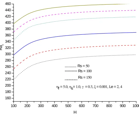
The variation of critical Rayleigh number with inter-phase heat transfer coefficient H for different parameter values is shown in figs 2 - 6. These figures indicate that the critical Rayleigh number increases from the LTE values when H is small to an LTNE values when H is large. Thus, the inter-phase heat transfer coefficient makes the system more stable for its intermediate values. Fig 2 indicates the effect of solute Rayleigh number on the critical Rayleigh number. For
small values of solute Rayleigh number (Rs ≤ 10) the convection sets is stationary mode. As the value of
Ra
c isincreased further the motion become significant and the convection sets. The critical Rayleigh number for stationary convection is found to increase with the solute Rayleigh number, indicating that the presence of additional diffusing component stabilizes the system towards the stationary convection.
Figure 3 displays the variation of the critical Rayleigh number with H for different values of the Lewis number. This figure indicates that the increasing values of Le, the critical Rayleigh number increases. The Lewis number has very negligible effect on the convection.
The variation of the critical Rayleigh number with H for different values of porosity modified conductivity ratio γ is
shown in figure 4 when all other parameters are fixed. From this figure it is observed that for small H,
Ra
c isindependent of γ and is close to the LTE case. Since small value of H, there is no significant transfer of heat between the phases and the onset of criterion is not affected by the properties of the solid phase. For large values of H, through the stability criterion is independent of H, the condition for the onset of convection is based on the mean properties of
the medium, and therefore the critical Rayleigh number is independent of γ.
The variation of critical Rayleigh number
Ra
cwith H for different valuesη
f as shown in the figure 5 We find that anincrease in the value of f
η
increases in the value ofRa
c indicating that the effect of increasing the thermal anisotropyparameter is to delay the onset of convection.
Figure 6 shows the variation of critical Rayleigh number with H for different values of thermal anisotropy
parameter
η
S. Its effect is found to be similar to that ofη
f. However, for small values of H,Ra
cis found to beindependent of
η
S. For increasing values of parameterη
S the convection is stabilized. The effect ofη
Sat small values2 4 6 8 10 0
100 200 300 400 500 600
Ra
c
ξ
ηf = 1.0, ηs= 5.0, Le = 4.0, Rs = 100, γ = 0.3, H = 0.0, 0.1, 1.0
Figure 1: Variation of critical Rayleigh number Rac withξ for various values
f H
100 200 300 400 500 600 700 800 900 1000 100
200 300 400 500 600 700 800
Ra
c
H
---ξ =0.5
... ξ = 1.0
____ξ = 1.5 Le = 4.0, γ =0.3, ηf = 5.0, ηs = 1.0, Rs = 10, 50
Figure 2: Variation of critical Rayleigh number Rac with H for different values
of ξ and Rs
100 200 300 400 500 600 700 800 900 1000
160 180 200 220 240 260 280 300 320 340 360 380 400 420 440 460
Ra
c
H ... Rs = 50
--- Rs = 100
_____Rs = 150
ηf = 5.0,ηs= 1.0, γ = 0.3, ξ = 0.001, Le = 2, 4
Figure 3: Variation of critical Rayleigh number Rac with H for different values
200 400 600 800 1000 100
200 300 400 500 600
Ra
c
H
--- Rs = 100
______ Rs = 200
Figure 4. Variation of critical Rayleigh number Rac with H for different
l f d R
ηf = 5.0, ηs = 1.0, ξ = 0.001, Le= 4.0, γ = 0.5, 0.3, 1.0
200 400 600 800 1000
0 50 100 150 200 250 300 350 400 450 500
Ra
c
H
ηs=1.0, Le = 4.0, γ = 0.3, ξ = 0.001, ηf = 10, 8, 5 ---Rs = 100
________Rs = 200
Figure 5: Variartion of critical Rayleigh number Rac with H for different
l f d R
200 400 600 800 1000
0 50 100 150 200 250 300 350 400
Ra
c
H _____Rs =100
---Rs =200
ηf =5.0, Le = 4.0, ξ= 0.001,γ = 0.3, ηs = 5 , 3, 1
Figure 6: Variation of critical Rayleigh number Rac with H for various values
ACKNOWLEDGEMENT
REFERENCES
1. Nilsen, T. and Storesletten, L., An analytical study of natural convection in isotropic and anisotropic porous
channels, Trans. ASME J. Heat Transfer, 112 (1990), 396-401.
4. Baytas. A. C, and Pop I., Free convection in a square porous cavity using a thermal nonequilibrium model,
International Journal of Thermal Science, 41(2002), 861-870.
5. Saeid H.Nawaf., Analysis of mixed convection in a vertical porous layer using non-equilibrium model.
International Journal of Heat and Mass Transfer. 47 (2004), 5619-5627.
6. Straughan. B., Global nonlinear stability in porous convection with a thermal non-equilibrium model.
Proceedings of the Royal Society, 462 (2010), 409-418.
7. Postelnicu, A. and Rees, D.A.S. The onset of Darcy-Brinkman convection in a porous layer using a thermal
non-equilibrium model- Part I: Stress free boundaries, International Journal of Energy Res. 27 (2003),
961- 973.
8. Malashetty, M. S., Shivakumara, I. S., and Kulkarni, S., 2005, The onset of convection in an Anisotropic
porous layer using a thermal non-equilibrium model. Transport in Porous Media, 60 (2005), 199–215.
9. Malashetty, M. S.and Rajashekhar Heera, Onset of double diffusive convection in a sparsely packed porous
layer using a thermal non-equilibrium model, Acta Mechanica, (2008), 8-36.
10. Balagondar, P.M., and Pranesha Setty A., A Study of natural convection in anisotropic porous rectangular
channels using a thermal non-equilibrium model. International Journal of Mechanics and Engineering
17(2012), 5-16.
Source of support: Nil, Conflict of interest: None Declared