Proceedings of the
Ninth International Workshop on
Graph Transformation and
Visual Modeling Techniques
(GT-VMT 2010)
Graph Algebras for Bigraphs
Davide Grohmann, Marino Miculan17 pages
Guest Editors: Jochen K ¨uster, Emilio Tuosto
Managing Editors: Tiziana Margaria, Julia Padberg, Gabriele Taentzer
Graph Algebras for Bigraphs
∗Davide Grohmann1, Marino Miculan2
1[email protected],2[email protected]
Department of Mathematics and Computer Science, University of Udine, Italy
Abstract: Binding bigraphs are a graphical formalism intended to be a meta-model for mobile, concurrent and communicating systems. In this paper we present an algebra oftyped graph termswhich correspond precisely to binding bigraphs over a given signature. As particular cases, pure bigraphs and local bigraphs are described by two sublanguages which can be given a simple syntactic characterization. Moreover, we give a formal connection between these languages andSynchronized Hyperedge Replacementalgebras and the hierarchical graphs used inArchitectural Design Rewriting. This allows to transfer results and constructions among for-malisms which have been developed independently, e.g., the systematic definition of congruent bisimulations for SHR graphs via the IPO construction.
Keywords:Bigraphs, graph grammars, types.
1 Introduction
Bigraphical Reactive Systems(BRSs) [Mil01] have been proposed as a promising meta-model for ubiquitous, mobile systems. The key feature of BRSs is that their states arebigraphs, semi-structured data which can represent at once both the (physical, logical) location and the connec-tions of the components of a system. The dynamics of the system is given by a set of rewrite rules on this semi-structured data.
Bigraphs have been successfully used for representing many domain-specific calculi and mod-els, from traditional programming languages, to process calculi for concurrency and mobility, from context-aware systems to web-service orchestration languages—see e.g. [JM03, LM06,
BDE+06,GM07,BGH+08]. In fact, many variants of bigraphs have been proposed: the original purebigraphs have been later generalized intobinding bigraphs, allowing also for name scoping; other variants have been proposed, such aslocal bigraphsused for studying theλ-calculus.
In this paper, we propose ageneral typed languagefor binding bigraphs, which we recall in Section2. More precisely, in Section3we define an algebra of typed graph terms, so that well-typed terms correspond to binding bigraphs, and congruence captures bigraphic equality; this interpretation and corresponding properties are exposed in Section4. Moreover, as we will show in Section5, the important subcategories of pure, local and prime bigraphs can be described by suitable sublanguages which can be given a simple and effective syntactic characterization.
Finally, we show how this language can be tailored to formalisms introduced in literature (for quite different purposes). In Section6we consider hypergraphs used inSynchronized Hyperedge Rewriting[FHL+05] and the “designs” ofArchitectural Design Rewriting[BLMT07].
∗Work funded by MIUR PRIN project “SisteR”, prot. 20088HXMYN.
Graph Algebras for Bigraphs
used to simulate a simple model of a mobile phone system.
Bigraphical reactive systems are related to general graph transformation systems; Ehrig et al. [10] provide a recent comprehensive overview of graph transformation systems. In particular, bigraph matching is related to the general graph pattern matching (GPM) problem, so general GPM algorithms might also be applicable to bigraphs [11, 14, 20, 21]. As an alternative to implementing matching for bigraphs, one could try to formalize bigraphical reactive systems as graph transformation systems and then use an existing implementation of graph transformation systems. Some promising steps in this direction have been taken [19], but they have so far fallen short of capturing precisely all the aspects of binding bigraphs. For a more detailed account of related work, in particular on relations between BRSs, graph transformations, term rewriting and term graph rewriting, see the Thesis of Damgaard [8, Section 6].
The remainder of this paper is organized as follows. In Section 2 we give an informal presentation of bigraphical reactive systems and in Section 3 we present our matching algorithm: we first recall the graph-based inductive char-acterization, then we develop a term-based inductive charchar-acterization, which forms the basis for our implementation of matching. In Section 4 we describe how our implementation deals with the remaining nondeterminism and in Sec-tion 5 we discuss a couple of auxiliary technologies needed for the implementaSec-tion of the term-based matching rules. In Section 6 we finally describe the BPL Tool and present an example use of it. We conclude and discuss future work in Section 7.
2. Bigraphs and Reactive Systems
In the following, we present bigraphs informally; for a formal definition, see the work by Jensen and Milner [13] and Damgaard and Birkedal [9].
2.1. Concrete Bigraphs
A concrete binding bigraph Gconsists of aplace graph GP and a link graph GL. The place graph is an ordered list of trees indicatinglocation, with rootsr0,...,rn, nodesv0,...,vk, and a number of special leavess0,...,smcalled
sites, while the link graph is a general graph over the node set v0,...,vk extended with inner names x0,...,xl, and equipped with hyper edges, indicatingconnectivity.
We usually illustrate the place graph by nesting nodes, as shown in the upper part of Figure 1 (ignore for now the interfaces denoted by “ :· →·”). Alinkis a hyper edge of the link graph, either an internaledge eor aname y. Links
BigraphG:�3,[{},{},{x0,x2}],X� → �2,[{y0},{}],Y�
0
1
2
y0 y1 y2
x0 x2
x1
e2
v0
v1
v2 v3
e1
X={x0,x1,x2}
Y={y0,y1,y2}
Place graphGP: 3→2
roots:
sites:
r0
v0
v1
s0
v2
r1
v3
s2 s1
Link graphGL:X→Y
names:
inner names:
y0 y1 y2
v0
v1
v2
v3
x0 x2 x1
e1
e2
Fig. 1. Example bigraph illustrated by nesting and as place and link graph.
2
Figure 1: A binding bigraph (picture taken from [BDGM07]).
These results are useful for several reasons. First, the typed algebra we propose can be used as a language for binding, pure, local and prime bigraphs, alternative to the bigraph algebra [JM03]. Moreover, we confirm once more that bigraphs are a quite expressive general framework of ubiquitous systems. These connections pave the way for transferring results and constructions from bigraphs to the SHR and ADR frameworks, and vice versa, as suggested in Section7.
2 Binding Bigraphs
In this section we recall Milner’sbinding bigraphs[JM03,JM04]. Intuitively, a binding bigraph represents an open system, so it has an inner and an outer interface to “interact” with subsystems and the surrounding environment (Figure1). Thewidthof the outer interface describes theroots, that is, the various locations containing the system components; the width of the inner interface describes thesites, that is, the holes where other bigraphs can be inserted. On the other hand, the
namesin the interfaces describe free links, that is end points where links from the outside world can be pasted, creating new links among nodes. In particular, we consider binding bigraphs with (possibly) multiply localized names, as in [Mil04] and slightly generalizing [JM03,JM04].
More formally, let K be abinding signature of controls (i.e., node types), and ar: K →
N×Nbe the arity function. The arity pair(h,k)(writtenh→k) consists of thebinding arity h
and thefree arity k, indexing respectively the binding and the free ports of a control.
Definition 1(Interfaces) Aninterfaceis a pairhm,Xiwheremis a finite ordinal (calledwidth),
X is a finite set of names. Abinding interfaceis a triplehm,loc,Xi, wherehm,Xiis an interface andloc⊆m×X is a localitymap associating a subset of the names in X with sites in m. If
Sometime, we shall represent the locality map as a vector~X= (X0,...,Xm−1)of subsets, where
Xs is the set of names local tos; thusX\~X=X\(X0∪ ··· ∪Xm−1) are the global names. We call an interfacelocal(resp.global) if all its names are local (resp. global). We denote by]the union of already disjoint sets, i.e.,S]T ,S∪T ifS∩T =/0, otherwise it is undefined.
Definition 2(Pure and binding bigraphs) A(pure) bigraph G:hm,Xi → hn,Yiis composed by aplace graph GPand alink graph GLdescribing node nesting and (hyper-)links among nodes:
G= (V,E,ctrl,GP,GL):hm,Xi → hn,Yi (pure bigraph) GP= (V,ctrl,prnt):m→n (place graph)
GL= (V,E,ctrl,link):X→Y (link graph)
whereV,E are the sets of nodes and edges respectively;ctrl:V →K is thecontrol map,which assigns a control to each node; prnt:m]V →V]nis the (acyclic)parent map(often written also as<);link:X]P→E]B]Y is thelink map,whereP=∑v∈Vπ1(ar(ctrl(v)))is the set of ports and B=∑v∈Vπ2(ar(ctrl(v))) is the set of bindings (associated to all nodes). A link
l∈X]Pisboundiflink(l)∈B; it isfreeiflink(l)∈Y]E.
Abinding bigraph G:hm,loc,Xi → hn,loc0,Yiis a (pure) bigraphGu:hm,Xi → hn,Yi
satis-fying the following locality conditions:
1. if a link is bound, then the names and ports linked to it must lie within the node that binds it; 2. if a link is free, with outer namex, thenxmust be located in every region that contains any
inner name or port of the link.
Definition 3(Binding bigraph category) The category of binding bigraphs over a signatureK
(writtenBbg(K)) has local interfaces as objects, and binding bigraphs as morphisms.
Given two binding bigraphs G:hm,loc,Xi → hn,loc0,Yi, H:hn,loc0,Yi → hk,loc00,Zi, the
compositionH◦G:hm,loc,Xi → hk,loc00,Ziis defined by composing their place and link graphs,
whenever they have disjoint node and edge sets:
1. the composition ofGP:m→nandHP:n→kis defined as HP◦GP= (V
G]VH,ctrlG]ctrlH,(idVG]prntH)◦(prntG]idVH)):n→k;
2. the composition ofGL:X→Y andHL:Y →Zis defined as HL◦GL= (V
G]VH,EG]EH,ctrlG]ctrlH,(idEG]linkH)◦(linkG]idPH)):X→Z.
Definition 4(Pure, local and prime bigraphs) The category ofpure bigraphs(Big) is the full subcategory ofBbgwhose objects are of the formhn,(/0),Xi(often shorten ashn,Xi).
The category oflocal bigraphs(Lbg) is the full subcategory of binding bigraphs whose objects are of the formhn,(~X),S~
Xi(often shorten as(~X)).
The category ofprime bigraphs(Pbg) is the full subcategory of local bigraphs whose objects are of the formhn,(~X),S~Xi, withn∈ {0,1}, (often shorten as before:(~X)).
An important operation about (bi)graphs, is the tensor product. Intuitively, the tensor prod-uct puts “side by side” two bigraphs, givenG:hm,(~X),Xi → hn,(~Y),YiandH:hm0,(~X0),X0i →
hn0,(~Y0),Y0i, their tensor product is a bigraphG⊗H:hm+m0,(X~~X0),X∪X0i → hn+n0,(~Y~Y0),Y∪
Y0idefined when global names inX,X0andY,Y0are disjoint. Two useful variants of tensor
prod-uct can be defined using tensor and composition: theparallel productk, which merges shared names between two bigraphs, and theprime product|, that also merges all roots in a single one. As shown in [Mil04,DB06], all bigraphs can be constructed by composition and tensor product from a set ofelementary bigraphs:
• 1 :h0,(/0),/0i → h1,(/0),/0iis the barren (i.e., empty) root;
• mergen:hn,(/0),/0i → h1,(/0),/0imergesnroots into a single one;
• γm,n,(~X,~Y):hm+n,(~X~Y),(S~X)∪(S~Y)i → hm+n,(~Y~X),(S~X)∪(S~Y)ipermutes the firstm
roots having local names in~X with the followingnroots with local names in~Y. • /x:h0,(/0),{x}i → h0,(/0),/0iis aclosure, that is it mapsxto an edge;
• y/X:h0,(/0),Xi → h0,(/0),{y}isubstitutes the names inX withy, i.e., it maps the whole set
X toy; as a shortcuts, we write~y/~X to meany0/X0⊗...⊗yn−1/Xn−1;
• pXq:h1,(X),Xi → h1,(/0),Ximeans that names inX are switched from local to global
• conversely,(X):h1,(/0),Xi → h1,(X),Xilocalizes the global names ofX.
• Finally,K~x(~X):h1,(X),/0i → h1,(/0),~xiis a control which may contain other graphs, and it has
free ports linked to the name in~x, whilst the names~X are connected to its binding ports. We use the convention that local names are enclosed in parenthesises.
Bigraphs can be given always in discrete normal form: the idea of this normal form is to separate wirings (i.e., linkings) from discrete bigraphs (i.e., nesting of nodes). The following is an easy generalization of [DB06, Theorem 1] to the case of bigraphs with multiply located names.
Theorem 1(Discrete Normal Form (DNF)) 1. Any binding bigraph G:I→ hn,~YB,(S~YB)]YFican be expressed as
G=N
i<n(~yi)/(~Xi)⊗Ni<|YF|wi/Wi⊗ N
i<|Z|(/zi◦zi/Zi)
◦D
where D:I→ hm,~X,(S~
X)]W]Ziis a name discrete.
2. Any name discrete D:I→ hm,~X,(S~X)]W]Zican be expressed as
D=α⊗((P0⊗...⊗Pn−1)◦π)
whereα is a renaming, andπa permutation.
3. Any name-discrete prime P:J→ h1,(UB),Uican be expressed as
(UB)◦(mergen+k⊗idU)◦(pα0q⊗...⊗pαn−1q⊗M0⊗...⊗Mk−1)◦π
where every Mi:Ji→ h1,(/0),UiMiis a free discrete molecule, and for renamingsαi:Vi→UiC, we have U = (U
i∈nUiC)]Ui∈kUiM.
(a) l x0x1...xn
...
(b) L
A
y0 y1 ym
...
x0 x1... xn
... ...
...
Figure 2: Example of an atomic label (a) and a non-atomic one (b).
3 Graph Grammar for Bigraphs
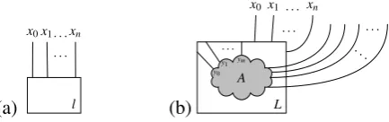
In this section we introduce a language for binding bigraphs. It is parametric over a ranked alphabet of labelsL = (La,Ln,exit:La∪Ln→N,in:Ln→N), whereLa are theatomic
labels, ranged over byl, andLnare thenon-atomiclabels, ranged over byL. Each label is given
anexit-rank,exit(l)∈N, enumerating the “exiting tentacles”. Non-atomic labels have anin-rank
in(L)∈N, enumerating the label’s “incoming tentacles”. We often denote byL the setLa∪Ln.
One may think of a node with an atomic labellas an hyperedge withexit(l)tentacles, as in Figure2(a). A node labelled withLhasexit(L)tentacles, and may contain a subsystem whose exiting tentacles are either linked to the in(L)ports of the node, or go “outside” the node, see Figure2(b). More formally, the language of graphs is as follows.
Definition 5(Agent graphs) LetN be an infinite set of names,V be an infinite set of variables, andL be a ranked alphabet of labels. Anagent-graph Ais a term generated as follows:
A::=ε|0|l(~x)|L(~x)[A\~y]|X|A|A|AkA|νz.A|A[w7→z]|A•|z|A|•z where~x,~y⊆N∗;l∈L
a,L∈Lnwithexit(l) =exit(L) =|~x|,in(L) =|~y|;X∈V; andw,z∈N.
Moreover, in a termA, eachX is used at most once.
Intuitively,ε represents the absence of any system, that is, no agents at all, while0represents an empty agent (i.e., an agent with no nodes). We denote byl(~x) atomic hyperedges whose tentacles are linked to the names in~x, whilst byL(~x)[A\~y]non-atomic hyperedges having exiting tentacles linked to the names in~x, containing a subgraphAwhose names~yare linked on the edge itself. Graph variablesXare needed for representing open systems, i.e., graphs with holes.
Two agent graphsA,Bcan be composed in parallel in two different ways:A|B“merges” two graphs into a unique one (i.e., in the same location), whileAkBputs the two systems side by side, i.e., they keep living in different locations.
As usual,νy.Alimits the scope ofytoA, whileA[w7→z]is the explicit substitution of namew
withz. Notice that the agent-graphA[w7→z]exhibits the namezalso whenwdoes not appear in
A; in this case, the operator [w7→z]“creates” unused (or idle) names.
Finally,A•|z localizes zto (the location of)A. This means thatzcan only be accessed by/linked to nodes lying in the location ofA, that is, they must be inside or in parallel (|) toA. Dually,A•|z
globalizes z, allowing a localized name to be used also by nodes in different locations.
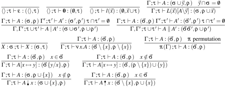
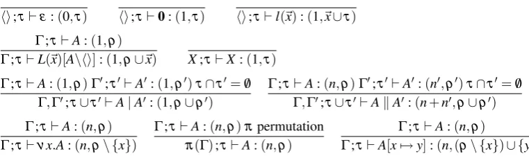
hi;τ`ε:(hi,τ) hi;τ`0:(/0,τ) hi;τ`l(~x):(/0,~x∪τ)
Γ;τ`A:(σ∪~y,ρ) ~y∩σ=/0 Γ;τ`L(~x)[A\~y]:(σ,ρ∪~x)
Γ;τ`A:(σ,ρ)Γ0;τ0`A0:(σ0,ρ0)τ∩τ0=/0
Γ,Γ0;τ∪τ0`A|A0:(σ∪σ0,ρ∪ρ0)
Γ;τ`A:(σ~,ρ)Γ0;τ0`A0:(~σ0,ρ0)τ∩τ0=/0
Γ,Γ0;τ∪τ0`AkA0:(~σ~σ0,ρ∪ρ0)
X:σ;τ`X:(σ,τ)
Γ;τ`A:(~σ,ρ) Γ;τ`νx.A:(~σ\ {x},ρ\ {x})
Γ;τ`A:(~σ,ρ) πpermutation π(Γ);τ`A:(~σ,ρ)
Γ;τ`A:(~σ,ρ) x∈~σ
Γ;τ`A[x7→y]:(~σ{y/x},ρ)
Γ;τ`A:(~σ,ρ) x∈/~σ
Γ;τ`A[x7→y]:(~σ,(ρ\ {x})∪ {y})
Γ;τ`A:(σ,ρ∪ {x}) x∈/ρ Γ;τ`A|•x:(σ∪ {x},ρ)
Γ;τ`A:(~σ,ρ) x∈~σ Γ;τ`A|•x:(~σ\ {x},ρ∪ {x})
Figure 3: Type inference rules for agent-graphs.
Definition 6(Type system for agent graphs) Simple typesτ,σ,ρ are finite sets of names. Anagent-type(~τ,τ)is a pair formed by a list~τ=τ0...τn−1of simple types (wherehiis the empty list), and a simple-typeτ, such thatτ∩(τ0∪...∪τn−1) =/0.
Anenvironmentis a pairΓ;τformed by a list of typed variables (Γ=~X:~τ=X0:τ0,...,Xn−1:
τn−1) and a simple-type (τ), such that(~τ,τ)is an agent-type.
A typing judgement is of the formΓ;τ`A:(~σ,ρ), whose inference rules are in Figure3.
Agent-types(~τ,τ) = (τ0...τn−1,τ)describe both the locations of a graph, and the names that the graph exposes to the environment. Names in τ are “global”, and can be used from every location; instead, names inτican be used only inside thei-th location of the system.
We are interested in open systems, that is systems with “holes”. An environmentΓ;τ=X0:
τ0,...,Xn−1:τn−1;τdeclares the “inner interface” of an agent: the names of the variables (Xifor i∈n), with their sets of local names (τiare the names local toXi), and the set of incoming global
names (τ), i.e., names that can be used from within any variable.
Notation. List concatenation is denoted simply by juxtaposition. We extend the operators ∈, ∪ and\ over set lists as follows: x∈~τ iff there exists ¯τ ∈~τ such that x∈τ¯; let S be a set, thenτ0...τn−1∪S,(τ0∪S)...(τn−1∪S)andτ0...τn−1\S,(τ0\S)...(τn−1\S).Γ1,Γ2is the concatenation ofΓ1andΓ2, defined when dom(Γ1)∩dom(Γ2) = /0. We introduce some useful shortcuts:ν~x.A=νx|~x−1|....νx0.A;A[~x7→~y] =A[x07→y0]...[xn−17→yn−1]when|~x|=|~y|=n;
A[X 7→x] =A[x07→x]...[x|X|7→x]ifX6= /0,A[/07→x] =A[z7→x]for somezfresh (i.e.,zis not
used byA); finallyA[~X7→~x] =A[X07→x0]...[Xn−17→xn−1]when|~X|=|~x|=n.
Some intuitive explanation of the typing rules may be useful. Empty agents have only global names, as defined by the environment. Notice that0is the null process, whichisan agent, while
l Xx z
x w
u
l0 Yx
L y
y
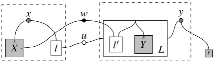
Y:{x},X:{x,z};{y} `νu.((l(x,u)|X)|•z[z7→w]kL(y,u)[(Y|l0(w,x))\x]•|w):({w}{w},{x,y})
Figure 4: An example of an agent-graph.
The names exposed by a composition (|) of two subgraphs are the union of the names exposed by the two subgraphs. The rule forkis quite similar, but in this case the two graphs keep their different locations, and hence the names can be treated in a different way, so global names are the union of agents’ global names, whilst local names remains unchanged, i.e, the two lists of local names are concatenated. If a variable has typeσ in an environmentΓ, then it exposesσ local names and the global namesτ defined by the environment. The restriction deletes a name from the set of global or local exposed names. The next rule describes the possibility to reorder the variables in the environment; it will be important in the definition of a category for agent-graphs. For the substitutionA[w7→z]there are two cases: (1) ifwis localized, it will be substituted byz; (2) if it is global the substitution (possibly) deleteswand addszto the set of global names. Notice that ifw,zare not used inA, then it effectively adds the namezto its interface.
An example of an agent-graph is given in Figure 4, where white nodes are closed (that is, nodes not accessible from the context); the other are the external nodes (which can be visible by a context): the grey nodes are global and the black ones are local.
Now, we can prove the following properties on our language.
Proposition 1 IfΓ;τ`A:(σ~,τ)andΓ;τ`A:(~σ0,τ0)then~σ =~σ0 andτ=τ0.
Lemma 1(substitution lemma) The following rule is admissible.
Γi;τi`Ai:(σi,ρi) 0≤i<n ∀i6= j.τi∩τj=/0 X0:σ0,...,Xn−1:σn−1;Sin=−01ρi`A:(~η,ζ) Γ0,...,Γn−1;Sin=−01τi`A{A0/X0,...,An−1/Xn−1}:(~η;ζ)
As happens often with graph grammars, the same system may be denoted by many terms. Therefore, it is convenient to introduce astructural congruenceover terms, capturing graph iso-morphisms up-to free nodes. Congruence judgments are of the formΓ;τ`A≡B, forA,Bterms of the language. This turns our language into agraph algebra, whose axioms are in AppendixA.
Proposition 2 LetΓ;τ`A≡A0,Γ;τ`A:(σ~,ρ)if and only ifΓ;τ `A0:(~σ,ρ).
4 Interpreting Agent Graphs as Binding Bigraphs
Definition 7 The categoryA(L)of agent-graphs, over a ranked alphabetL, has graph types
(~σ,ρ) as objects, and judgments on agent-graphs as morphisms, that is, ifX0:η0,...,Xn−1:
ηn−1;τ `A:(~σ,ρ) then (X0,...,Xn−1,A):(~η,τ)→ (~σ,ρ) is a morphism. Composition is defined in virtue of Lemma1.
Proposition 3 (A(L),k,hi; /0`ε:(hi,/0))is a strict symmetric monoidal category.
4.1 Interpretation of agent-graphs as binding bigraphs
LetL be a ranked alphabet of labels; we define a functor from the agent-graph categoryA(L)
to the binding bigraph categoryBBg(KL), for a suitable bigraphical signatureKL. The idea
is to map agent-graph hyperedges into nodes, and nodes (or names) into links (i.e., outer names and edges); hence, the bigraphical signature corresponds to the alphabet of labels. Formally:
KL ,{l: 0→exit(l)|l∈La} ∪ {L:in(L)→exit(L)|L∈Ln}.
We can now define the functorJ−K:A(L)→BBg(KL)by induction on the typing judgments:
Objects: J(~σ,τ)K=h|~σ|,~σ,τi
Morphisms: Jhi;τ`ε :(hi,τ)K=idτ
Jhi;τ`0:(/0,τ)K=1kidτ
Jhi;τ`l(~x):(/0,~x∪τ)K=l~xkidτ
JΓ;τ`L(~x)[A\~y]:(σ,ρ∪~x)K=L~x,(~y)◦JΓ;τ`A:(σ∪~y,ρ)K
JX:σ;τ`X:(σ,τ)K=id(σ)kidτ
JΓ,Γ
0;τ∪τ0`A|A0:(σ∪σ0,ρ∪ρ0)
K=JΓ;τ `A:(σ,ρ)K|JΓ
0;τ0`A0:(σ0,ρ0) K
JΓ,Γ
0;τ∪τ0`AkA0:(~σ~σ0,ρ∪ρ0)
K=JΓ;τ `A:(~σ,ρ)KkJΓ
0;τ0`A0:(~σ0,ρ0) K
JΓ;τ `νx.A:(~σ\ {x},ρ)K=/(x)◦JΓ;τ`A:(σ~,ρ)K (ifx∈~σ)
JΓ;τ`νx.A:(σ~,ρ\ {x})K=/x◦(JΓ;τ`A:(~σ,ρ)Kk {x}) (ifx∈/~σ)
JΓ;τ `A[x7→y]:(~σ{y/x},ρ)K= (y)/(x)◦JΓ;τ`A:(~σ,ρ)K (ifx∈~σ)
JΓ;τ `A[x7→y]:(~σ,(ρ\ {x})∪ {y})K=y/x◦(JΓ;τ`A:(~σ,ρ)Kk {x}) (ifx∈/~σ)
JΓ;τ`A•|x:(σ∪ {x},ρ)K= (x)◦JΓ;τ `A:(σ,ρ∪ {x})K
JΓ;τ`A|
•x:(~σ\ {x},ρ∪ {x})
K=pxq◦JΓ;τ`A:(~σ,ρ)K (ifx∈~σ)
Jπ(Γ);τ`A:(~σ,ρ)K=JΓ;τ`A:(~σ,ρ)K◦π.
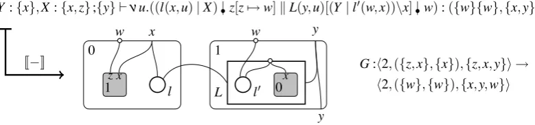
Basically, each variable of typeσ is encoded as a site havingσ local names; therefore, variable permutation is site permutation. Restricted names are represented by bigraph edges, not accessi-ble from the context. The graph0is represented by the empty root 1. An example is in Figure5.
Now we can prove thatJ−Krespects the structure of the two categories:
Proposition 4 J−K:(A(L),k,hi; /0`ε :(hi,/0))→(Bbg(K),k,id(0,/0,/0))is strict monoidal.
Moreover, the axiomatization of the graph algebra given in AppendixAis sound and complete with respect to bigraph equivalence.
Proposition 5 Let A,A0 be two agent-graphs; then, for every environmentΓ;τ: Γ;τ`A≡A0
Y:{x},X:{x,z};{y} `νu.((l(x,u)|X)|•z[z7→w]kL(y,u)[(Y|l0(w,x))\x]•|w):({w}{w},{x,y})
1z x l 0
w x
0x
l0
L
1
w
y y
G:h2,({z,x},{x}),{z,x,y}i → h2,({w},{w}),{x,y,w}i J−K
Figure 5: An example of encoding an agent-graph into a binding bigraph.
4.2 Representing binding bigraphs with agent-graphs
In this section we show that our language is expressive enough to cover all binding bigraphs, over a given signatureK. To this end, we define a translation from binding bigraphs to agent-graphs of a language whose ranked labels are defined by means of the bigraphical signature.
LK ,({k|k: 0→n∈K,atomic},{k|k:m→n∈K,non atomic},exit,in)
exit(k),n fork:m→n∈K in(k),m fork:m→n∈K non atomic
The representation function L−M maps objects of the category Bbg(K) to agent-types, as
Lhn,(~X),(
S~
X)]XiM ,(~X,X). In order to simplify the translation of bigraphs, in virtue of
Theorem1 we can suppose w.l.o.g. that all binding bigraphs are in discrete normal form. Let
G:hm,~XB,(S~XB)]XFi → hn,~YB,(S~YB)]YFi, be in discrete normal form as follows
G=N
i<n(~yi)/(~Xi)⊗Ni<|YF|wi/Wi⊗ N
i<|Z|(/zi◦zi/Zi)
◦(~a/~b⊗((P0⊗...⊗Pn−1)◦π))
then, forQ~ =Q0,...,Qm−1a list ofmvariables, we define
LGMQ~ =νz|Z|−1....νz0. (Lp0M~Qk...kLpn−1MQ~)
[~b7→~a][W07→w0]...[W|YF|−17→w|YF|−1][~X07→~y0]...[~Xn−17→~yn−1]
wherep0⊗...⊗pn−1= (P0⊗...⊗Pn−1)◦π◦(v0(X0)⊗...⊗v(mX−m1−1)).
Given p= (UB)◦(mergeh+k⊗idU)◦(p~a0/~b0q⊗...⊗p~ah−1/~bh−1q⊗m0⊗...⊗mk−1), then
LpM~Q= LK
0
~x0,(~S0)◦p0MQ~ |...|LK ki−1
~xki−1,(~Ski−1)◦pki−1M~Q|
Lv j0
(Xj0)M~Q[~b07→~a0]•|~a0|...|Lv jhi−1
(Xjhi−1)MQ~[~bhi−17→~ahi−1]•|~ahi−1
|
•UB
Lv i
(Xi)M~Q=Qi
LK~x,(/0)◦1M~Q=K(~x) where Katomic
LK~x,(~S)◦pM~Q=K(~x)[LpM~Q[~S7→~s]\~s] where Knon-atomic, and~sfresh
where the nodes v0,...,vm−1 have special controls not present in K, and they are used only to simplify the translation. In practice, these special nodes give a “name” to each hole of the bigraphs, i.e., the nodevi represents thei-hole of the bigraphs. Notice that, the hole sequence
1z x l 0
w x
0x
l0
L
1
w
y y
G:h2,({z,x},{x}),{z,x,y}i → h2,({w},{w}),{x,y,w}i
0
v1
x
1
v0
z x
y
L−M
Q0:{x},Q1:{x,z};{y} `
νz.((((l(x,z)|Q1)kε)•|zk(L(y,z)[(Q0|l0(w,x))[x7→s]\s]kε)|•w)[z7→w]):({w}{w},{x,y})
Figure 6: An example of encoding a binding bigraph into an agent-graph.
Proposition 6 Let G:hm,~XB,(S~XB)]XFi → hn,~YB,(S~YB)]YFibe a binding bigraph. Then,
LGMQ~ is an agent-graph s.t.Q~ :~XB;XF `LGM~Q:(~YB,YF), andJ~Q:~XB;XF `LGM~Q:(~YB,YF)K=G.
We can also establish nice connections between the axiomatizations of the two categories.
Proposition 7 Let G,G0:hm,~X
B,(S~XB)]XFi → hn,~YB,(S~YB)]YFibe two binding bigraphs over a given signature. Then, G=G0 if and only if~Q:~XB;XF `
LGM~Q≡LG0M~Q.
Proposition 8 ForΓ;τ`A:(~σ,ρ)a typing judgment:Γ;τ`LJΓ;τ `A:(~σ,ρ)KMdom(Γ)≡A.
These results induces anormal formfor agent-graphs inspired to the discrete normal form of binding bigraphs. This normal form tries to separate the notions of nesting and linking:
A≡ν~z.(A¯0k...kA¯n−1)[~X7→~x]
¯
A≡ L0(~x0)[A¯0[~Y07→~y0]\~y0]|...|Lm−1(~xm−1)[A¯m−1[~Ym−17→~ym−1]\~ym−1]|
l0(~z0)|...|lk−1(~zk−1)|X0[~Z07→~z0]•|~z0| ··· |Xh−1[~Zh−17→~zh−1]•|~zh−1•|W.
Proposition 9 Every agent-graph is structural equivalent to an agent-graph in normal form.
Finally, notice that the mappingL−M:Bbg(K)→A(LK)is not a functor, because the
com-position of wirings in binding bigraphs is not respected by the graph comcom-position defined in virtue of Lemma1. Therefore,Bbg(K)andA(LK)are not isomorphic. However, as we will
see next, composition is respected in the important subcategories of pure and local bigraphs.
5 Characterizing pure, local and prime bigraphs
(A,k,hi; /0`ε:(hi,/0))
(P,k,hi; /0`ε: /0) (L,k,hi `ε:hi) (H,|,`ε: /0)
(Bbg,k,idh0,/0,/0i)
(Big,k,idh0,/0i) (Lbg,k,id()) (Pbg,|,id/0) J−K L−M
J−K L−M J−K L−M J−K L−M Π
U
Figure 7: Relations among the categories under investigation.
hi;τ`ε:(0,τ) hi;τ`0:(1,τ) hi;τ`l(~x):(1,~x∪τ)
Γ;τ`A:(1,ρ)
Γ;τ`L(~x)[A\hi]:(1,ρ∪~x) X;τ`X:(1,τ)
Γ;τ`A:(1,ρ)Γ0;τ0`A0:(1,ρ0)τ∩τ0=/0 Γ,Γ0;τ∪τ0`A|A0:(1,ρ∪ρ0)
Γ;τ`A:(n,ρ)Γ0;τ0`A0:(n0,ρ0)τ∩τ0=/0 Γ,Γ0;τ∪τ0`AkA0:(n+n0,ρ∪ρ0)
Γ;τ`A:(n,ρ)
Γ;τ`νx.A:(n,ρ\ {x})
Γ;τ`A:(n,ρ)πpermutation π(Γ);τ`A:(n,ρ)
Γ;τ`A:(n,ρ)
Γ;τ`A[x7→y]:(n,(ρ\ {x})∪ {y})
Figure 8: Typing rules for restricted agent-graphs where all names are global.
subcategories are covered by the same sublanguage, obtained by removing•|and•|:
A::=ε|0|l(~x)|L(~x)[A\~y]|X|A|A|AkA|νz.A|A[w7→z]. (1) Despite we use the same (sub)language, and essentially the same typing rules of Figure3, we are able to describe both pure and local bigraphs, just by restricting the form of types and typing en-vironment. Figure7summarizes the correspondences among the categories under investigation.
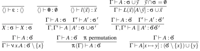
5.1 Pure bigraphs
In pure bigraphs all names are global, hence, variables and agents cannot have localized names. Therefore, a typing system for pure bigraphs is derivable from the system in Figure3by simply restricting to types of the form(~/0,τ), while the variables in the environment can have only /0 as type. The only function of~/0 is to count the locations of the system. Therefore, takingn=|~/0|, a typing judgement is simply of the formΓ;τ`A:(n,ρ)whereAis a term as per (1). We can hence defineglobal type (n,ρ)is a pair wheren∈Nandρ is a simple types; an environment
Γ;τ is a list of variablesΓ=~X =X0,...,Xn−1, together with a simple-typeτ.
Notice that forLnon-atomic, it must bein(L) =0, because there are no local names which can be linked to an in-tentacle. This is enforced by the typing system, which is given Figure8. These rules are essentially the same of Figure3, just with the restricted form of types and environments.
Definition 8 The categoryP(L)of agent-graphs, over a ranked alphabetL, has types(m,ρ)
as objects, and judgments as morphisms, i.e., ifX0,...,Xn−1;τ`A:(m,ρ)then(X0,...,Xn−1,A): (n,τ)→(m,ρ)is a morphism. Composition is defined in virtue of Lemma1.
hi `ε:hi hi `0: /0 hi `l(~x):~x
Γ`A:σ∪~y ~y∩σ=/0
Γ`L(~x)[A\~y]:σ∪~x
X:σ`X:σ
Γ`A:σ Γ0`A0:σ0 Γ,Γ0`A|A0:σ∪σ0
Γ`A:~σ Γ0`A0:~σ0 Γ,Γ0`AkA0:~σ~σ0
Γ`A:~σ
Γ`νx.A:~σ\ {x}
Γ`A:~σ πpermutation π(Γ)`A:~σ
Γ`A:~σ
Γ`A[x7→y]:(~σ\ {x})∪ {y}
Figure 9: Typing rules for restricted agent-graphs where all names are local.
The encoding functorJ−K:Big(K)→L(PK)and the representation functionL−M:P(K)→
Big(KL)are particular cases of the ones for binding bigraphs. Again the two maps establish a
bijection between the two categories.
5.2 Local bigraphs
In local bigraphs all names are localized, hence there are no global names, and variables can have only their own names. So, the typing is obtained again from the system in Figure3by simply restricting to types of the form(~σ,/0), while in the environment the set of the global names is always /0. More formally, a typing judgement is of the formΓ`A:~σwhereAis a term generated by the grammar (1), alocal type~τ=τ0...τn−1 is a list of simple types, and anenvironment Γ is a list of typed variables (Γ=~X:~τ=X0:τ0,...,Xn−1:τn−1). The type inference rules are in Figure9. Notice that, in local bigraphs, non-atomic hyperedges can have non-zero in-rank.
Definition 9 The category L(L) of agent-graphs, over a ranked alphabetL, has local types ~σ as objects, and judgments as morphisms, that is, if X0 :τ0,...,Xn−1 :τn−1 `A :~σ then (X0,...,Xn−1,A):~τ →~σis a morphism. Composition is defined in virtue of Lemma1.
Proposition 11 (L(L),k,hi `ε:hi)is a strict symmetric monoidal category.
The two encoding functorsJ−K:Lbg(K)→L(LK), andL−M:L(K)→Lbg(KL)are
par-ticular cases of the ones for binding bigraphs. Notice that, in this parpar-ticular case,L−Mis actually
a functor; and, as before, the two functors establish a bijection between the two categories.
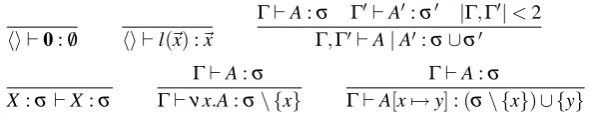
5.3 Prime bigraphs
Following the idea of the functorJ−Kfrom agent-graph to bigraphs, we can identify a
subcate-gory ofA, where all agents have zero or one variable. These areprime bigraph, that is bigraphs with at most one hole. One may think of these bigraphs as single-located (open) systems.
We can characterize pure prime bigraphs by a restriction on agent types. A typing judgement is of the formΓ`A:σwhereAis a one-variable term generated byA::=0|l(~x)|X|A|A|νz.A|
A[w7→z]. Aprime typeσ is a simple type, and an environmentΓis a list of typed variables of at most length one, i.e.,Γ::=hi |X:ρ. The induced type inference rules are in Figure10.
hi `0: /0 hi `l(~x):~x
Γ`A:σ Γ0`A0:σ0 |Γ,Γ0|<2 Γ,Γ0`A|A0:σ∪σ0
X:σ`X:σ
Γ`A:σ
Γ`νx.A:σ\ {x}
Γ`A:σ
Γ`A[x7→y]:(σ\ {x})∪ {y}
Figure 10: Typing rules for restricted agent-graphs with one locality.
i.e., ifX :τ `A:ρ then(X,A):τ →ρ is a morphism or ifhi `A:ρ then(hi,A): /0→ρ is a morphism. Composition is defined as follows:
Γ`A:τ X :ρ`A0:ρ Γ`A0{A/X}:ρ
Proposition 12 (H,|,hi `0: /0)is a strict symmetric monoidal category.
The two encoding functorsJ−K:Pbg(K)→H(LK)andL−M:H(L)→Pbg(LK)can be
defined as a “simplification” of the ones for local bigraphs.
Proposition 13 Let A,A0be terms; then, for every environment X:τ: X:τ`A≡A0if and only
ifJX:τ`A:τ0K=JX :τ`A0:τ0K.
Proposition 14 Let H,H0 :(hi)→(Y) be two prime graphs; then, H=H0 iff hi `
LHMhi ≡
LH0Mhi. Instead, if H,H0:(X)→(Y), then H=H0iff Q:X`LHMQ≡LH0MQ.
Forgetting localities. Let us consider only atomic signaturesKa, that is, where all controls
are atomic, and hence there is no nesting of nodes. In this case, we can define a functorU : Lbg(Ka)→Pbg(Ka)which “forgets” the localities of a local bigraph, merging all roots into a
single one and all sites (holes) into a single one. Formally: Objects:U((X0...Xn−1)) =X0+···+Xn−1.
Morphisms:U((V,E,ctrl,prnt,link)) = (V,E,ctrl,prnt0,link)whereprnt0(v) =0, for allv.
The previous functors J−K,L−M and the forgetful functorU induce a forgetful functor Π:
L(LKa)→H(LKa), defined as follows:
Objects:Π(σ0...σn−1) =σ0+···+σn−1.
Morphisms: given a graph in normal formA≡ν~z.(A¯0k...kA¯n−1)[~X7→~x]
, where every subgraph ¯Ai≡ l0i(~zi0)|...|lkii−1(~ziki−1)|X0i[~Z0i 7→~z0i]| ··· |Xhii−1[~Zhii−17→~zihi−1]
, then
Π(A) =ν~z. (l00(~z00)|...|lk00−1(~z0k0−1))|...|(l0n−1(~zn0−1)|...|lnk−1 n−1−1(~z
n−1
kn−1−1))|
X[~Z0
07→~z00]...[~Zh00−17→~z0h0−1]...[~Z0n−17→~zn0−1]...[~Zhnn−−11−17→~zhnn−−11−1]
In practice the above functor merges all the separate agent-graphs into a single-located graph. It translates akoperator with the|one and unifies all variables into a single one.
Proposition 15 Let~X :~τ`A:ρ=Π(Γ`B:~σ); then,~X :~τ`LU(JΓ`B:~σK)M~X ≡A.
Proposition 16 1. Let P:(~X)→(Y)be a prime bigraph, thenJQ~ :~X`LPM~QK=P.
2. Let~X :~τ`A:σ be a term, then~X :~τ`LJ~X :~τ`A:σKM~X ≡A.
6 Comparing with SHR hypergraphs and ADR designs
Our language for binding bigraphs can be used for capturing formalisms introduced in literature, often for quite different purposes. Here we consider the hypergraphs used inSynchronized Hy-peredge Rewriting(SHR) [FHL+05] and the “designs” ofArchitectural Design Rewriting(ADR)
[BLMT07]. Both are derived from the algebra of graphs introduced first in [CMR94].
SHR hypergraphs. SHR is a framework that allows hypergraph transformations by means of local productions replacing a single hyperedge by a generic hypergraph, possibly with constraints given by the surrounding nodes. The global rewriting is obtained by combining different local production whose conditions are compatible (with respect to some synchronization model).
In this paper, we are interested only in SHR hypergraphs, which are inductively defined as:
G::=0|l(~x)|G|G|νx.G
where0is the empty graph, the hyperedgelis linked to the nodes in~x, andνbindsxinG. Clearly, the SHR grammar is a particular case of the one for prime bigraphs (Section5.3), and specifically when the variable and substitutions are dropped.
ADR designs. ADR graphs (calleddesigns) resemble SHR graphs, but they have a notion of graph nesting, as some hyperedges can contain other graphs. Such nesting is used forincremental modelling, that is, edges can be refined into graphs or vice versa graphs collapse into edges. The ADR designs are inductively defined as:
D::=L[λ~x.G] G::=0|x|l(~x)|G|G|νx.G|D(~x)
where0is the empty graph, the hyperedgelis linked to the nodes in~x,νbindsxinG,D(~x)is a design generated by attaching designDto nodes~x, and finallyL[λ~x.G]represent a designL, with “body graph”Gand exposing the names~xin its interface.
The grammar of designs recalls the one defined for local bigraphs, when thekcomposition is omitted. In such a case, we deal with graphs residing in only one location. A formal translation of the ADR design grammar into the grammar in (1) can be defined as follow:
T(0) =0 T(x) =0[z7→x] (zfresh) T(G1|G2) =T(G1)|T(G2)
T(l(~x)) =l(~x) T(νx.G) =νx.T(G) T(L[λ~x.G](~y)) =L(~y)[G\~x]
7 Conclusion
In this paper we have first defined an algebra of typed term graphs which corresponds precisely to binding bigraphs, on a given signature. Secondly, we have shown that particular sublanguages of our main language properly characterize interesting subclasses of bigraphs, more precisely: pure and local bigraphs. Moreover, on this last kind of bigraphs we also give a reduced language for dealing with one-location (bi)graphs, named prime bigraphs. So, those languages can be used in place of the more complex bigraph algebra already present in literature. A family of bigraphical calculi has been introduced in [DK08]; however, these calculi has been suitably restricted for modelling biological systems and do not cover all possible bigraphs over a given signature.
Finally, it turns out that these languages are strictly connected with two well-know formalisms:
Synchronized Hyperedge Replacementhypergraphs, which can be represented as a sublanguage of the algebra for prime bigraphs (over atomic signatures), andArchitectural Design Rewriting
designs, which are a sub-case of the local bigraphs’ language.
A possible future work is to take advantage of the rich theory provided by bigraphical reactive systems [JM03], in order to obtain interesting results about SHR and ADR. In particular, we hope to generalize the transitions allowed in SHR graphs, which only rewrites a single hyperedge, to more general ones dealing with (sub)graphs. Moreover, bigraphs allow to synthesise labelled transition systems out of rewriting rules, via the so-calledidem-pushout construction [LM00]; it is important to notice that the bisimilarity induced by this labelled transitions system (LTS) is always a congruence. Therefore, given a reactive system over SHR (ADR) graphs, we can derive the labelled transition system in bigraphs, and remap it on SHR (ADR) graphs. Then, the inductive definition of SHR (ADR) agents can be useful for defining an SOS-like presentation of the LTS derived in this way.
Acknowledgments.We thank Emilio Tuosto and Ivan Lanese for useful discussions about SHR.
Bibliography
[BDE+06] L. Birkedal, S. Debois, E. Elsborg, T. Hildebrandt, H. Niss. Bigraphical Models of
Context-Aware Systems. In Aceto and Ing´olfsd´ottir (eds.),Proc. FoSSaCS. Lecture Notes in Computer Science 3921, pp. 187–201. Springer, 2006.
[BDGM07] L. Birkedal, T. C. Damgaard, A. J. Glenstrup, R. Milner. Matching of Bigraphs.
Electr. Notes Theor. Comput. Sci.175(4):3–19, 2007.
[BGH+08] M. Bundgaard, A. J. Glenstrup, T. T. Hildebrandt, E. Højsgaard, H. Niss.
Formal-izing Higher-Order Mobile Embedded Business Processes with Binding Bigraphs. In Lea and Zavattaro (eds.), COORDINATION. Lecture Notes in Computer Sci-ence 5052, pp. 83–99. Springer, 2008.
[CMR94] A. Corradini, U. Montanari, F. Rossi. An Abstract Machine for Concurrent Modular Systems: CHARM.Theor. Comput. Sci.122(1&2):165–200, 1994.
[DB06] T. C. Damgaard, L. Birkedal. Axiomatizing Binding Bigraphs. Nord. J. Comput.
13(1-2):58–77, 2006.
[DK08] T. C. Damgaard, J. Krivine. A Generic Language for Biological Systems based on Bigraphs. Technical report TR-2008-115, IT University of Copenhagen, Dec. 2008. [FHL+05] G. L. Ferrari, D. Hirsch, I. Lanese, U. Montanari, E. Tuosto. Synchronised
Hyper-edge Replacement as a Model for Service Oriented Computing. In Boer et al. (eds.),
Proc. FMCO. Lecture Notes in Computer Science 4111, pp. 22–43. Springer, 2005. [GM07] D. Grohmann, M. Miculan. Reactive Systems over Directed Bigraphs. In Caires and Vasconcelos (eds.), Proc. CONCUR 2007. Lecture Notes in Computer Sci-ence 4703, pp. 380–394. Springer, 2007.
[JM03] O. H. Jensen, R. Milner. Bigraphs and transitions. InProc. POPL. Pp. 38–49. 2003. [JM04] O. H. Jensen, R. Milner. Bigraphs and mobile processes (revised). Technical
re-port UCAM-CL-TR-580, Computer Laboratory, University of Cambridge, 2004. [LM00] J. J. Leifer, R. Milner. Deriving Bisimulation Congruences for Reactive Systems.
In Palamidessi (ed.), Proc. CONCUR. Lecture Notes in Computer Science 1877, pp. 243–258. Springer, 2000.
[LM06] J. J. Leifer, R. Milner. Transition systems, link graphs and Petri nets.Mathematical Structures in Computer Science16(6):989–1047, 2006.
[Mil01] R. Milner. Bigraphical Reactive Systems. In Larsen and Nielsen (eds.), Proc. 12th CONCUR. Lecture Notes in Computer Science 2154, pp. 16–35. Springer, 2001. [Mil04] R. Milner. Bigraphs whose names have multiple locality. Technical report 603,
Uni-versity of Cambridge, CL, Sept. 2004.
A Structural congruence
The free name function f nis defined as follows with respect to an environment(Γ,τ).
f nΓ;τ(ε) =τ f nΓ;τ(L(~x)[A\~y]) = (f nΓ;τ(A)\~y)∪~x∪τ f nΓ;τ(0) =τ f nΓ;τ(A1|A2) =f nΓ;τ(A1)∪f nΓ;τ(A2) f nΓ;τ(l(~x)) =~x∪τ f nΓ;τ(A1kA2) =f nΓ;τ(A1)∪f nΓ;τ(A2) f nΓ;τ(νy.A) = f nΓ;τ(A)\ {y} f nΓ;τ(A[w7→z]) = (f nΓ;τ(A)\ {w})∪ {z} f nΓ;τ(A•|x) = f nΓ;τ(A) f nΓ;τ(A•|x) =f nΓ;τ(A)
In the following table, the structural congruence for agent-graph is defined with respect to some environmentΓ;τ.
Γ ; τ ` A | 0 ≡ A Γ ; τ ` A1 | A2 ≡ A2 | A1 Γ ; τ ` ( A1 | A2 ) | A3 ≡ A1 | ( A2 | A3 ) Γ ; τ ` A k ε ≡ A Γ ; τ ` ε k A ≡ A Γ ; τ ` ( A1 k A2 ) k A3 ≡ A1 k ( A2 k A3 ) Γ ; τ ` ν x . 0 ≡ 0 if x / ∈ fnΓ ; τ ( 0 ) Γ ; τ ` ν x . ε ≡ ε if x / ∈ fnΓ ; τ ( ε ) Γ ; τ ` ν x . ν y . A ≡ ν y . ν x . A Γ ; τ ` ν x . A ≡ ν y . ( A { y / x } ) if y / ∈ fnΓ ; τ ( A ) Γ ; τ ` A [ x 7→ y ] ≡ ( A { z / x } )[ z 7→ y ] if z / ∈ fnΓ ; τ ( A ) Γ ; τ ` A [ x 7→ x ] ≡ A if x ∈ fnΓ ; τ ( A ) Γ ; τ ` A [ x 7→ y ] ≡ A if x / ∈ fnΓ ; τ ( A ) ∧ y ∈ fnΓ ; τ ( A ) Γ ; τ ` A [ x 7→ y ][ w 7→ z ] ≡ A [ w 7→ z ][ x 7→ y ] if x 6 = z , y 6 = w Γ ; τ ` A [ x 7→ y ][ y 7→ z ] ≡ A [ x 7→ z ] if y / ∈ fnΓ ; τ ( A ) Γ ; τ ` ν y . ( A [ x 7→ y ]) ≡ ν x . A if y / ∈ fnΓ ; τ ( A ) Γ ; τ ` ν z . ( A [ x 7→ y ]) ≡ ( ν z . A )[ x 7→ y ] if z / ∈ { x , y } Γ ; τ ` A |• x | • x ≡ A if x ∈ fnΓ ; τ ( A ) Γ ; τ ` A | • x |• x ≡ A if x ∈ fnΓ ; τ ( A ) Γ ; τ ` A |• x [ x 7→ y ] ≡ A [ x 7→ y ] |• y Γ ; τ ` A |• x [ y 7→ z ] ≡ A [ y 7→ z ] |• x if y 6 = x ∧ z 6 = x Γ ; τ ` A | • x [ x 7→ y ] ≡ A [ x 7→ y ] | • y Γ ; τ ` A | • x [ y 7→ z ] ≡ A [ y 7→ z ] | • x if y 6 = x ∧ z 6 = x Γ ; τ ` ν x . ( A |• x ) ≡ ν x . A if x ∈ fnΓ ; τ ( A ) Γ ; τ ` ν y . ( A |• x ) ≡ ( ν y . A ) | • x if x 6 = y Γ ; τ ` ν x . ( A | • x ) ≡ ν x . A if x ∈ fnΓ ; τ ( A ) Γ ; τ ` ν y . ( A | • x ) ≡ ( ν y . A ) | • x if x 6 = y Γ ; τ ` ν x . ( A1 | A2 ) ≡ ν x . A1 | A2 if x / ∈ fnΓ ; τ ( A2 ) Γ ; τ ` ν x . ( A1 k A2 ) ≡ ν x . A1 k A2 if x / ∈ fnΓ ; τ ( A2 ) Γ ; τ ` ν x . ( A1 k A2 ) ≡ A1 k ν x . A2 if x / ∈ fnΓ ; τ ( A1 ) Γ ; τ ` ( A1 | A2 )[ x 7→ y ] ≡ A1 [ x 7→ y ] | A2 if x / ∈ fnΓ ; τ ( A2 ) Γ ; τ ` ( A1 | A2 )[ x 7→ y ] ≡ A1 [ x 7→ y ] | A2 [ x 7→ y ] Γ ; τ ` ( A1 k A2 )[ x 7→ y ] ≡ A1 [ x 7→ y ] k A2 if x / ∈ fnΓ ; τ ( A2 ) ∧ x ∈ fnΓ ; τ ( A1 ) Γ ; τ ` ( A1 k A2 )[ x 7→ y ] ≡ A1 k A2 [ x 7→ y ] if x / ∈ fnΓ ; τ ( A1 ) ∧ x ∈ fnΓ ; τ ( A2 ) Γ ; τ ` ( A1 k A2 )[ x 7→ y ] ≡ A1 [ x 7→ y ] k A2 [ x 7→ y ] if x ∈ fnΓ ; τ ( A1 ) ∩ fnΓ ; τ ( A2 ) Γ ; τ ` ( A1 k A2 )[ x 7→ y ] ≡ A1 [ x 7→ y ] k A2 [ x 7→ y ] if x / ∈ fnΓ ; τ ( A1 ) ∪ fnΓ ; τ ( A2 ) Γ ; τ ` ( A1 | A2 ) |• x ≡ A1 |• x | A2 if x ∈ fnΓ ; τ ( A1 ) ∧ x / ∈ fnΓ ; τ ( A2 ) Γ ; τ ` ( A1 | A2 ) |• x ≡ A1 |• x | A2 |• x if x ∈ fnΓ ; τ ( A1 ) ∩ fnΓ ; τ ( A2 ) Γ ; τ ` ( A1 | A2 ) | • x ≡ A1 | • x | A2 if x ∈ fnΓ ; τ ( A1 ) ∧ x / ∈ fnΓ ; τ ( A2 ) Γ ; τ ` ( A1 | A2 ) | • x ≡ A1 | • x | A2 | • x if x ∈ fnΓ ; τ ( A1 ) ∩ fnΓ ; τ ( A2 ) Γ ; τ ` ( A1 k A2 ) | • x ≡ A1 | • x k A2 if x ∈ fnΓ ; τ ( A1 ) ∧ x / ∈ fnΓ ; τ ( A2 ) Γ ; τ ` ( A1 k A2 ) | • x ≡ A1 k A2 | • x if x / ∈ fnΓ ; τ ( A1 ) ∧ x ∈ fnΓ ; τ ( A2 ) Γ ; τ ` ( A1 k A2 ) | • x ≡ A1 | • x k A2 | • x if x ∈ fnΓ ; τ ( A1 ) ∩ fnΓ ; τ ( A2 ) Γ ; τ ` l ( ~ x )[ x 7→ z ] ≡ l ( ~ x ) { z / x } if x ∈ ~ x Γ ; τ ` L ( ~ x )[ A \ ~ y ] ≡ L ( ~ x )[ ( A { z / y } ) \ ( ~ y { z / y } )] if x ∈ ~ y ∧ z / ∈ ~ y ∪ fnΓ ( A ) Γ ; τ ` ν z . L ( ~ x )[ A \ ~ y ] ≡ L ( ~ x )[ ( ν z . A ) \ ~ y ] if z / ∈ ~ x ∪ ~ y Γ ; τ ` L ( ~ x )[ A \
~Y][x
7→ w ] ≡ L ( ~ x { w / x } )[ A \ ~ y ] if x ∈ ~ x ∧ w / ∈ ( fnΓ ( A ) \ ~ y ) Γ ; τ ` L ( ~ x )[ A \ ~ y ][ w 7→ z ] ≡ L ( ~ x )[ ( A [ w 7→ z ]) \ ~ y ] if w / ∈ ~ x ∪ ~ y ∧ z / ∈ ~ y Γ ; τ ` L ( ~ x )[ A [ w 7→ y ] \ ~ y ] ≡ L ( ~ x )[ A \ ( ~ y { w / y } ] if y ∈ ~ y ∧ w / ∈ fnΓ ; τ ( A ) Γ ; τ ` L ( ~ x )[ A \ ~ y ] |• z ≡ L ( ~ x )[ ( A |• z ) \ ~ y ] if z / ∈ ~ x ∪ ~ y Γ ; τ ` L ( ~ x )[ A \ ~ y ] | • z ≡ L ( ~ x )[ ( A |
• z)
![Fig. 1. Example bigraph illustrated by nesting and as place and link graph.Figure 1: A binding bigraph (picture taken from [BDGM07]).](https://thumb-us.123doks.com/thumbv2/123dok_us/7811526.2086156/3.595.91.420.144.372/example-bigraph-illustrated-nesting-figure-binding-bigraph-picture.webp)