AUSTRALIAN JOURNAL OF BASIC AND
Open Access Journal
Published BY AENSI Publication
© 2016 AENSI Publisher All rights reserved
This work is licensed under the Creative Commons Attribution International License (CC BY).http://creativecommons.org/licenses/by/4.0/
ToCite ThisArticle: Judi K. Nasjono, Mohammad Bisri, Agus Suharyanto and Dian Sisinggih., Regional Distribution of Frequency Fitted for East Java using Regional Flood Analysis Frequency.
Regional Distribution of Frequency Fitted for East Java using Regional
Flood Frequency Analysis
1Judi K. Nasjono, 2Mohammad Bisri, 3Agus Suharyanto
1Civil Engineering Department, University of Nusa Cendana, Kupang, Indonesia 2
Water Resources Engineering Department, University of Brawijaya, Malang, Indonesia 3Civil Engineering Department, University of Brawijaya, Malang, Indonesia
Address For Correspondence:
Judi K. Nasjono,Civil Engineering Department, University of Nusa Cendana, Kupang, Indonesia E-mail:[email protected]
A R T I C L E I N F O
Article history:
Received 12 February 2016 Accepted 18 March 2016 Available online 20 April 2016
Keywords:
Indonesia is a developing country. Currently,water infrastructure development gets so much attention. In the process of planning and design of water infrastructure development such as dams, bridges, and irrigation canals, an accurate estimate of the peak o
or underestimation of flood peak will affect the loss of the structure itself, the environment, and human life. Ideally, flood estimates are derived by selecting suitable frequency di
streams. However, as construction of the infrastructure is urgent, often the development is in the river without measurement. Therefore, hydrologists in Indonesia often apply indirect methods such as the methods of
and Synthetic UnitHydrograph for analyzing flood frequency. Overcoming the lack of data, Regional Flood
countries (Haddad and Rahman, 2012). This method
ungauged site. Index floodmethod is the method most widely applied in the al., 2001). This method analyzes data on
(Noto and La Loggia, 2009). The curve can be used to estimate the flood site in the same region. In the process of
area withhomogeneous hydrological statistic catchmentdiverse. This leads as to seethat
The process of determining a homogeneous area is called regionalization. Regionalization consists of two stages. First, it is pooling gauged sites into the region and identification of homogeneity of the region formed. Region can be based on administrative
(Castellarinet al., 2001). However,
Srinivas, 2003) as factors that affect the occurrence of floods are
common approaches in delineating regions for regional flood frequency is based on clustering techniques (Noto and La Loggia, 2009). In cluster techniques,
AUSTRALIAN JOURNAL OF BASIC AND
APPLIED SCIENCES
ISSN:1991-8178 EISSN: 2309-8414 Journal home page: www.ajbasweb.com
© 2016 AENSI Publisher All rights reserved
This work is licensed under the Creative Commons Attribution International License (CC http://creativecommons.org/licenses/by/4.0/
Judi K. Nasjono, Mohammad Bisri, Agus Suharyanto and Dian Sisinggih., Regional Distribution of Frequency Fitted for East Java using Regional Flood Analysis Frequency. Aust. J. Basic & Appl. Sci., 10(8): 106-113, 2016
Regional Distribution of Frequency Fitted for East Java using Regional
Analysis
Agus Suharyanto and2Dian Sisinggih
Department, University of Nusa Cendana, Kupang, Indonesia Water Resources Engineering Department, University of Brawijaya, Malang, Indonesia Civil Engineering Department, University of Brawijaya, Malang, Indonesia
Civil Engineering Department, University of Nusa Cendana, Kupang, Indonesia.
A B S T R A C T
Regional flood frequency analysis has been applied to the area of East Java. Regional division has been done through hierarchical clustering techniques. Regional identification is homogenous with discordancy measure and heterogeneity test base of L-Moment statistic and produces five homogeneous regions and one heterogeneous region. Each homogeneous region has unique growth curve. Dominant distribution in the region is Generalized Logistics and Generalized Pareto.
INTRODUCTION
Indonesia is a developing country. Currently,water infrastructure development gets so much attention. In the process of planning and design of water infrastructure development such as dams, bridges, and irrigation canals, an accurate estimate of the peak of flood in river and occurrence of intervals is required. Overestimation or underestimation of flood peak will affect the loss of the structure itself, the environment, and human life. Ideally, flood estimates are derived by selecting suitable frequency distribution with measurement data on river streams. However, as construction of the infrastructure is urgent, often the development is in the river without measurement. Therefore, hydrologists in Indonesia often apply indirect methods such as the methods of
for analyzing flood frequency.
Overcoming the lack of data, Regional Flood Frequency is a popular method and has been applied in many countries (Haddad and Rahman, 2012). This method generally estimates statistics on gauged
loodmethod is the method most widely applied in the Regional Flood Frequency analyzes data on gauged site to produce a standardized curve named as growth curve a Loggia, 2009). The curve can be used to estimate the flood design in gauged site and ungauged
process of data transfer, it is assumed that gauged site and withhomogeneous hydrological statistics. This assumption is necessary
This leads as to seethat homogeneous areas have similarity in distribution of flood frequency. The process of determining a homogeneous area is called regionalization. Regionalization consists of two stages. First, it is pooling gauged sites into the region and identification of homogeneity of the region formed. Region can be based on administrative boundaries, exiting geographical, or by
However, there is no universally accepted objective method (RamachandraRao and ffect the occurrence of floods are not yet fully understood. Nevertheless, common approaches in delineating regions for regional flood frequency is based on clustering techniques (Noto
luster techniques, hierarchical clustering is one of the widely
Judi K. Nasjono, Mohammad Bisri, Agus Suharyanto and Dian Sisinggih., Regional Distribution of Frequency Fitted
Regional Distribution of Frequency Fitted for East Java using Regional
flood frequency analysis has been applied to the area of East Java. Regional division has been done through hierarchical clustering techniques. Regional identification is homogenous with discordancy measure and heterogeneity test base of and produces five homogeneous regions and one heterogeneous region. Each homogeneous region has unique growth curve. Dominant distribution in the region is Generalized Logistics and Generalized Pareto.
Indonesia is a developing country. Currently,water infrastructure development gets so much attention. In the process of planning and design of water infrastructure development such as dams, bridges, and irrigation f flood in river and occurrence of intervals is required. Overestimation or underestimation of flood peak will affect the loss of the structure itself, the environment, and human life. stribution with measurement data on river streams. However, as construction of the infrastructure is urgent, often the development is in the river without measurement. Therefore, hydrologists in Indonesia often apply indirect methods such as the methods of rational
hydrology. Ward’s method is most frequently used (Lin and Chen, 2006) and recommended by (Hosking and Wallis, 1997). Usually the process of delineating is based on physiographic characteristics such as catchment area, rainfall, length of the main river, the slope of the main river, and river discharge. Once the region is formed, they can be tested for homogeneity. Test homogeneity statistic based L-moment is widely used in regional flood frequency (Hussain, 2011) and has several advantages compared to other methods (Viglioneet al., 2007).
The importance of choosing the frequency distribution that matches the nature of the river flow has attracted a lot of attention. Haddad and Rahman (2011) investigate and select distribution for Tasmania, Richard M. Vogel et al. (1993a, b) for Australia and the United States, Ellouze and Abida, (2008) for Tunisia, and Karim and Chowdhury (1995) compared four distributions in Bangladesh. Many statistical distributions for flood frequency have been introduced in hydrological literature including Extreme Value Type 1 (Gumbel), General Extreme Value, Normal, Lognormal, Gamma, Exponential, and Log Pearson Type 3. Practitioners in East Java apply only Gumbel Distribution and Log Pearson Type 3, fitted to sample data, and one that gives the best fit is selected.
The objective of this paper is to identify the frequency distribution best fit to the data for regional flow in East Java of Indonesia. To our best knowledge, there have been no previous studies to select the best fit for regional flood frequency distribution in East Java.
MATERIAL AND METHOD
To achived the objective, we considered using cluster techniques of Ward’s method and test homogeneity based L-moment in regionalization,thenfive different distributions having three parametersfitted on regions formed. Criteria for selection of the frequency distribution are comparable procedures of skewness and L-kurtosis and goodnes of fit test.
Watershed Grouping:
Cluster analysis is part of multivariate statistical analysis to divide objects into groups. In this regional analysis, factors of latitude, longitude, contributing area, circumference, length of the main rivers, elevation gauged site, discharge, rainfall, river slope, runoff coefficient, and Topographic Wetness Index are considered to be analyzed. As those factors have different units, standardizationis necessary, with a range from zero to one. With this technique, a site can be combined with others based on similar data. In hierarchical cluster, the similarity of data on the sites, which will be combined into groups (clusters),is measured from the smallest value between the sites based on Euclidean equation. Cluster relationships formed subsequently are analyzed using Ward equation that measures the degree of similarity of each cluster, until all sites combined into one cluster only. The results of cluster analysis in the form of dendogram present a picture of how the site merged into one cluster only. The decision on how many groups or regions formed is made using the pattern of similarity change or distance value that changes at every stage of cluster formation. In stage where a big change in similarity happens, then it is the for the cutting dendogram.
L-Moment:
L-moment is a statistical method that lately is used much in hydrological methods when dealing with regional flood frequency (Noto and La Loggia, 2009). L-moment is modified from its probability weighted moment (Greenwood et al., 1979, by Hosking, 1990). L-moment is an alternative to summarize the statistical properties of hydrological data (Karim and Chowdhury, 1995). Just like product moment ratio, that is coeficient of variation, skewness and kurtosis, Hosking (1990) defines L-moment ratio as follows:
L-CV (L-Coefficien of varians) = (1)
L-skewness = (2)
L-kurtosis = (3)
In which
= ∑ …… , = 0, 1, … , − 1 (4)
Australian Journal of Basic and Applied Sciences, 10(8) April 2016, Pages: 106-113 Discordancy test:
Hosking and Wallis (1997) laid the basis for the measurement of discordant of a region with n sites. At every site i Discordancy Measure is defined as follows:
# = $ % − %& '( % − %& (5)
in which u = ) *', %& = $ ∑ %+ , and ( = ∑+ , − ,- , − ,- '
This discordancy measure tes is useful to identify sites from formed region that gross discordant with that region as a whole and would be removed from that region. Irregularities are due to incorrect data values, outliers, trends, and shift in the mean of a sample that reflacted in L-moments of sample. Critical value of discordant usually depends on number of station in a region as given in tabular form (Hosking and Wallis, 1997).
Homogenity test:
Region formed based on similar physiographic needs acknowledgment of its homogeneity by heterogeneity size. The size of the sample is obtained by comparing the variability of L-moments ratio of sites in a region with expected variability in homogeneous region as defined by Hosking and Wallis (1993). The heterogeneity measured is defined as follows:
. = / 01
21 (6)
in whichVis weighted variance for L-CV
3 = ∑+ 4 − 56 / ∑+ (7)
The expected mean value (89) and standard deviation (:9) are obtained from repeated simulation of homogeneous region having same record of length n of site i, 5 is regional average L-CV. Following Hosking and Wallis (1997), the four-parameter of kappa distribution is used in simulation. A Monte Carlo simulated program is used to generates random data. The region is “acceptably homogeneous” if H< 1, “possibly heterogeneous” if 1 ≤ . < 2, and “definitely heterogeneous” is. > 2.
Selection on regional distribution:
The robust distribution for the region is identified based on goodness of best fit criteria. It aims is to identify a distribution among the available candidates which is the best fit to the sample data. The goodness of fit is judged by how well the L-skewness and L-kurtosis of the fitted. In this study, the L-moment ratio diagram and
>?@ AB> statistic criteria are used as the goodness-of-fit measures for identifying the robust regional distribution
as recommended (Hosking and Wallis 1997).
>?@ AB> statistic is defined as
?CDE' = FCDE'− 5+ H :⁄ (8)
In whichFCDE'isL-kurtosis of fitted distribution; H = $A J∑+A JJ 4 |J|− 56is the bias of 5; and :is the standard deviation of L-kurtosis regional ( 5) gained from several simulations ($A J) on a region with homogenous distribution candidates, with some frequency distribution candidates, and several sites having the same length of data with the sample data.
The smallest value of>?@ AB>on one distribution candidate makes the candidate as the true frequency distribution for that particular region. The fit is considered to be adequate if >?@ AB> statistic is sufficiently close to zero, a reasonable criterion being >?@ AB> ≤ 1.64. Probably, more than one distribution candidates that have
>?@ AB> less of the criterion, the one with the lowest >?@ AB>is regarded as the most appropriate distribution.
Studi Area and Data:
using the tool box of Quantum GIS. Catchment area of sites varies from 6.39 km2 to 956.45 km2. Perimeter varies from 14.03 km to 161.45. Main river slope varies from 0.03 to 0.61.
RESULT AND DISCUSSION
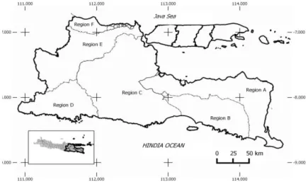
Officially, the study area was divided into six regions by the Indonesian government. Region name is given in Table 1 together with catchment areas and the characteristics of the statistics that are calculated using L-moment statistics. WS Bengawan Solo has 12 sites,and the critical value for discordancy statistic is 2.757; WS Brantas has 8 sites, and the critical value for discordancy statistic is 2.140; WS BondoyudoBedadunghas 5 sites, and the critical value discordancy statistic is for 1.333. Therefore, the data from these three regions is acceptable.WS WelangRejoso only has three sites, too few and uninformative according to Hosking and Wallis (1997), so it should be considered a new composition by using objective technique, that is the application of cluster.
Fig. 1: Delineation of Regions.
Fig. 2: Regional Growth Curve Fitted to Region A.
Six regions have been identified through cluster analysis but spatially multiple sites in a cluster arefar apart and surrounded by members of other clusters so subjective adjustment to the results of cluster analysis needs to be done. This modification is done to improve the geographical coherence and obtain homogeneous region as much as possible. Five regions have been identified as “possibly heterogeneous” i.e. Region A, Region B, Region C, Region D, and Region E; one region is “definitely heterogeneous” as shown in Table 2. Discordancy value in parentheses at sites in Region A is less than the critical value of the nine sites, i.e. 2.329; critical value of Region B is 1.333, Region C is 1.917, Region D is 1.648, Region E and F is 1. There is no discordant in each region. Figure 1 shows the location of the sixth region.
0.01 0.1 1 10
-1 0 1 2 3 4
q
Australian Journal of Basic and Applied Sciences, 10(8) April 2016, Pages: 106-113
Fig. 3: Regional Growth Curve Fitted to Region B.
Fig. 4: Regional Growth Curve Fitted to Region C.
Fig. 5: Regional Growth Curve Fitted to Region C.
Region A is a combination of WS WelangRejoso Region, WS BaruBajulmati, and WS PekalenSampean. Region B is a modification of WS BondoyudoBedandung. Borderline of Region A and Region B which extends from east to west is a series of volcanoes along the Island of Java. Region C is largely WS Brantas, the biggest watershed in East Java Province. Region D, Region E, and Region F divide WS Bengawan Solo into three.
In Region F, Gembul site is a site with the highest L-CV and L-skewness than other sites. Examination of the data of Gembul site found one-year reference with enormous value which requires an examination of the validity of the data. However,it is not easy to gain sufficient access for inspection, and then the data is retained.
0.1 1
-0.4 0.6 1.6 2.6 3.6 4.6
q
Gumbel, log(-log(1-1/T))
0.1 1
-0.4 0.6 1.6 2.6 3.6 4.6
q
Gumbel, log(-log(1-1/T))
0.001 0.01 0.1 1 10
0 0.5 1 1.5 2 2.5 3 3.5 4
q
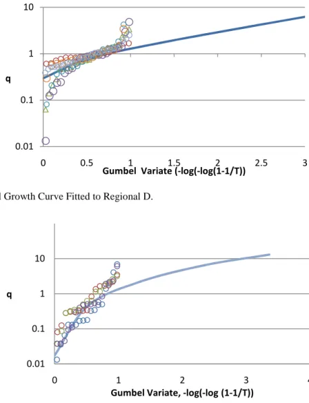
Fig. 6: Regional Growth Curve Fitted to Regional D.
Fig. 7: Regional Growth Curve Fitted to Regional E.
Rejososite is excluded from the formation of region. This site is the cause of heterogeneity of regions formed, leading to no suitablefrequency distribution. The flow of the river at this site is regulated streamflow.
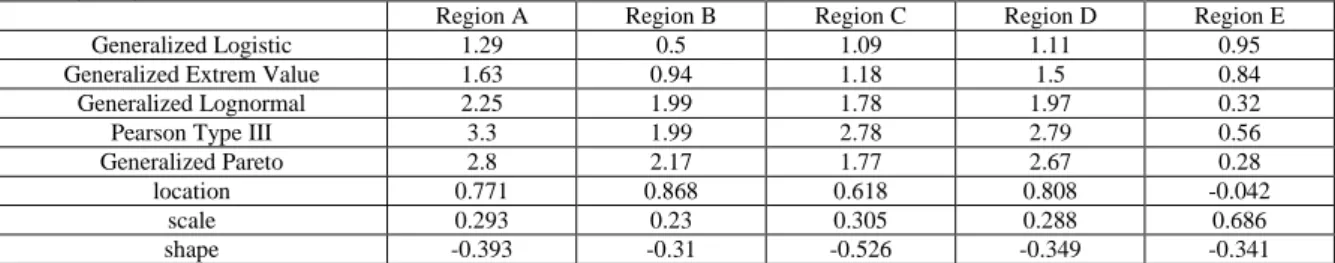
After ensuring homogeneity from the study area, the next step is to choose an appropriate frequency distribution for the regions. For the eastern part of Java, the distribution candidate is General Logistic (GLO), Generalized Extreme Value (GEV), Pearson type 3 (PIII), lognormal distribution (LN3), and Generalized Pareto (GPA), by 500 simulations for each region, the >?@ AB>has been calculated and is shown in Table 3. GEV and GLO are found to fit well to Region A base on the criterion of>?@ AB>, but the lowest is GLO. The same thing happened in Region B and Region C. GLO was found suitable for Region D. GPA is the lowest of four distributions to fit well to Region E.
GLO distribusion is identified as robust distribution for five region in study area, and GPA distribution is robust distribution for one region; therefore, regional distibution frequancy was developed using these distribution. The form of regional frequancy analisys for GLO distribution is expressed as follows:
O = P +QR 1 − ST − 1UR (9)
and GPA distribution is expressed as follows:
O = P +QRV1 − W1 −'XYZ (10)
qis growth factor; P, [,and\is parameter location, scale dan shape respectively; estimation value of each parameter can be seem in Table 3. The equation suitable with each region is presented as follows:
Region A
O = 0.771 − 0.75 1 − T − 1 . _ (11)
Region B
q = 0.868 − 0.742 1 − T − 1 . (12)
0.01 0.1 1 10
0 0.5 1 1.5 2 2.5 3
q
Gumbel Variate (-log(-log(1-1/T))
0.01 0.1 1 10
0 1 2 3 4
q
Australian Journal of Basic and Applied Sciences, 10(8) April 2016, Pages: 106-113
Region C
O = 0.618 − 0.58 1 − T − 1 .c (13)
Region D
O = 0.808 − 0.825 1 − T − 1 . _ (14)
Region E
O = −0.042 − 2.012 V1 − d1 −'e . Z (15)
Tabel 1: Cathments, L-Moment Ratio, Discordancy Measure and Region.
Sample
ID Site Name
Catchment Area
Sample
Size Mean Annual L -CV L-Skewness L-Kurtosis
Discordancy
Measure Region Name
(km2
) (year) (m3/s) t t3 t4 D (i)
1 Prumpung 102.52 13 4.56 0.3462 0.3819 0.1998 0.54
WS Bengawan Solo
2 Klero 40.53 13 9.43 0.3139 0.3972 0.4669 2.4
3 Ngilirip 92.11 15 24.41 0.3746 0.1456 -0.0687 1.46
4 Kerjo 55.66 17 32.51 0.6667 0.573 0.3891 0.31
5 Gembul 60.89 16 19.52 0.9363 0.8868 0.7339 1.97
6 Lamong 194.17 16 92.73 0.1981 0.4826 0.4371 1.77
7 Keang 139.57 18 25.58 0.1776 0.2876 0.1866 0.62
8 Gondang_M 63.15 17 63.15 0.7655 0.7018 0.4755 0.88
9 Gondang_S 66.65 15 40.61 0.5281 0.353 0.0812 0.68
10 Gangseng 55.44 15 32.43 0.5304 0.3551 0.116 0.49
11 Lorok 220.93 16 57.57 0.3096 0.459 0.4526 0.61
12 Grindulu 601.83 28 245.4 0.2776 0.2777 0.1626 0.26
13 Bagong 45.97 24 25.21 0.4231 0.3098 0.2216 0.6
WS Brantas
14 Keser 44.45 23 38.44 0.4732 0.3875 0.3814 1.06
15 Sumber_Ampel 6.39 14 11.4 0.5576 0.4386 0.3341 0.62
16 Cubanrondo 18.45 19 3.57 0.4067 0.3479 0.1752 1.47
17 Sayang 10.61 19 6.4 0.5894 0.5964 0.401 0.72
18 Duren 15.62 16 5.75 0.465 0.434 0.3755 0.4
19 Lahar 34.59 16 5.35 0.5736 0.4112 0.1906 1.43
20 Kadalpang 96.66 13 26.15 0.514 0.6797 0.4948 1.69
21 Rondoningo 80.46 18 19.38 0.3852 0.6323 0.5806 1
WS Pekalen Sampean
22 Deluwang 167.41 18 42.77 0.4815 0.4801 0.4565 1
23 Pekalen 168.73 28 43 0.2082 0.2753 0.2716 1
24 Sampean 647.84 17 73.76 0.39 0.3581 0.1532 1
25 Stail 286.82 18 66.89 0.3763 0.397 0.273 1
WS Baru Bajulmati
26 Tambong 117.85 18 31.73 0.5383 0.4436 0.2556 1
27 Baru 655.01 31 116.31 0.1684 0.1278 0.2426 1
28 Bomo Bawah 119.28 14 39.95 0.3192 0.2089 0.0583 1
29 Sanen 181.37 27 111.65 0.3734 0.246 0.1351 1.32
WS Bondoyudo Bedadung
30 Asem 143.24 25 25.29 0.2443 0.3714 0.3175 1.26
31 Bondoyudo 177.71 30 71.26 0.2773 0.4327 0.2646 0.96
32 Mujur 130.01 12 36.96 0.7693 0.8456 0.838 1.32
33 Bedadung 956.45 16 335.59 0.3288 0.4452 0.3271 0.14
34 Welang 164.41 18 16.06 0.278 0.1606 0.1607 1
WS Welang Rejoso
35 Rejoso 210.13 19 34.56 0.2267 0.057 0.2732 1
36 Kramat 191.11 20 61.83 0.5381 0.5785 0.4737 1
Table 2: Final Delineation of Regions and Region Statistic.
Region Site ID and Discordancy Measure (D) in Region 5 5 5 . . .
A 24(0.96); 25(0.14); 26(0.96); 28(0.77); 22(1.11); 36(0.74); 23(1.12); 21(1.75); 34(1.44) 0.3833 0.3925 0.3052 1.51 0.67 0.22 B 27(1.2); 29(1.27); 30(0.27); 33( 1.05); 31(1.21) 0.2712 0.31 0.2502 1.45 0.77 0.08 C 15(0.78); 16(0.49); 17(0.44); 20(1.13); 6(1.75); 19(0.67);
32(1.75) 0.5057 0.5263 0.3868 1.94 0.75
-0.06 D 7(0.91); 13(0.59); 14(1.38); 18(1.37); 11(1.23); 12(0.51) 0.3552 0.3487 0.282 1.71
-0.15 -0.68
E 8(1); 9(1); 10(1); 4(1) 0.6285 0.5046 0.2759 1.2 1.08 0.89
F 1(1); 2(1); 3(1); 5(1) 0.5119 0.4649 0.34 4.74 3.2 2.39
Table 3:>?@ AB> of Distribution and Parameter of the Best Fit Distribution in Each Homogenous Region.
Region A Region B Region C Region D Region E
Generalized Logistic 1.29 0.5 1.09 1.11 0.95
Generalized Extrem Value 1.63 0.94 1.18 1.5 0.84
Generalized Lognormal 2.25 1.99 1.78 1.97 0.32
Pearson Type III 3.3 1.99 2.78 2.79 0.56
Generalized Pareto 2.8 2.17 1.77 2.67 0.28
location 0.771 0.868 0.618 0.808 -0.042
scale 0.293 0.23 0.305 0.288 0.686
shape -0.393 -0.31 -0.526 -0.349 -0.341
Conclusions:
Six regions defined by the Indonesian government need to be modified in order to be acceptable to implement a regional frequency distribution. Based on data from screening, some regions simply have too few measuring stations that need to be merged. Selection on appropriate frequency distribution had been carried out based on appropriate statistical tests. Eastern part of Java Island is largely hydrologicallyhomogeneous. Region identified as heterogeneous is part of WS BengawanSolo covering parts of Central Java; thus, further research based on regional flood frequency analysis needs to be done. The methodology used in this study can be adopted for other regions in Indonesia if sufficient flood records are available.
ACKNOWLEDGMENT
Most of the data is obtained from the Center of Water Resource Research and Development Bandung, funded by the Directorate of Higher Education.
REFERENCES
Brath, A., A.Castellarin, M.Franchini, G.Galeati, 2001. Estimating the index flood using indirect methods. Hydrol. Sci. Sci. Hydrolo, 46: 399–418.
Castellarin, A., D.Burn, A.Brath, 2001. Assessing the effectiveness of hydrological similarity measures for flood frequency analysis. J. Hydrol, 241: 270–285. doi:10.1016/S0022-1694(00)00383-8
Ellouze, M., H.Abida, 2008. Regional Flood Frequency Analysis in Tunisia : Identification of Regional Distributions. Water Resour. Manag, 943–957. doi:10.1007/s11269-007-9203-y
Greenwood, J.A., J.M.Landwher, N.C.Matalas, 1979. Probability Weighted Moments: Definition and Relation to Parameters od Several Distributions Epressable in Invers Form. Water Resour. Res., 15: 1049–1054.
Haddad, K., A.Rahman, 2012. Regional flood frequency analysis in eastern Australia : Bayesian GLS regression-based methods within fixed region and ROI framework–Quantile Regression vs . Parameter Regression Technique. J. Hydrol, 430-431: 142–161. doi:10.1016/j.jhydrol.2012.02.012
Haddad, K., A.Rahman, 2011. Selection of the best fit flood frequency distribution and parameter estimation procedure : a case study for Tasmania in Australia. Stoch Env. Res Risk Assess, 25: 415–428. doi:10.1007/s00477-010-0412-1
Hosking, J.R.M., 1990. L-moments: Analysis and Estimtion of Distribution using Linier Combination of Order Statistics. J. R. Stat. Soc., 52: 105–124.
Hosking, J.R.M., J.R.Wallis, 1997. Regional frequency analysis. Cambridge University Press.
Hosking, J.R.M., J.R.Wallis, 1993. Some staistics useful in regional frequency analysis. Water Resour. Res., 29: 271–281.
Hussain, Z., 2011. Application of the Regional Flood Frequency Analysis to the Upper and Lower Basins of the Indus River , Pakistan. Water Resour. Manag, 25: 2797–2822. doi:10.1007/s11269-011-9839-5
Karim, A., J.U.Chowdhury, 1995. A comparison of four distributions used in flood frequency analysis in. Hydrol. Sci. J., 40: 55–66. doi:10.1080/02626669509491390
Lin, G., L.Chen, 2006. Identification of homogeneous regions for regional frequency analysis using the self-organizing map. J. Hydrol, 324: 1–9. doi:10.1016/j.jhydrol.2005.09.009
Noto, L.V., G.La Loggia, 2009. Use of L-moments approach for regional flood frequency analysis in Sicily, Italy. Water Resour. Manag, 23: 2207–2229. doi:10.1007/s11269-008-9378-x
Ramachandra Rao, A., V.V.Srinivas, 2003. Some problems in regionalization of watersheds, in: Water Avialability and Global Changes, pp: 301–308.
Viglione, A., F.Laio, P.Claps, 2007. A comparison of homogeneity tests for regional frequency analysis. WATER Resour. Res., 43: 1–10. doi:10.1029/2006WR005095
Vogel, R.M., T.A.McMahon, F.H.S.Chiew, 1993. Floodflow frequency model selection in Australia. J. Hydrol, 146: 421–449.