NUMERICAL EXPERIMENTS FOR THE ESTIMATION OF MEAN
DENSITIES OF RANDOM SETS
F
EDERICOC
AMERLENGHI1,V
INCENZOC
APASSO2,3 ANDE
LENAV
ILLAB
,21Dept. of Mathematics, Universit`a degli Studi di Pavia, via Ferrata 1, 27100 Pavia, Italy;2Dept. of Mathematics,
Universit`a degli Studi di Milano, via Saldini 50, 20133 Milano, Italy ;3Escuela Politecnica Superior, Universidad Carlos III de Madrid, Av. de la Universidad 30 28911 Leganes, Spain
e-mail: [email protected], [email protected], [email protected]
(Received November 13, 2013; revised February 25, 2014; accepted April 24, 2014)
ABSTRACT
Many real phenomena may be modelled as random closed sets inRd, of different Hausdorff dimensions. The
problem of the estimation of pointwise mean densities of absolutely continuous, and spatially inhomogeneous, random sets with Hausdorff dimensionn<d,has been the subject of extended mathematical analysis by the authors. In particular, two different kinds of estimators have been recently proposed, the first one is based on the notion of Minkowski content, the second one is a kernel-type estimator generalizing the well-known kernel density estimator for random variables. The specific aim of the present paper is to validate the theoretical results on statistical properties of those estimators by numerical experiments. We provide a set of simulations which illustrates their valuable properties via typical examples of lower dimensional random sets.
Keywords: density estimator, Hausdorff dimension, Hausdorff measure, kernel estimate, Minkowski content, random closed set, stochastic geometry.
INTRODUCTION
Given an Euclidean spaceRd,the problem of the evaluation and estimation of the mean density of lower dimensional random closed sets (i.e., with Hausdorff dimension less than d), such as fiber processes, boundaries of germ-grain models,n-facets of random tessellations, and surfaces of full dimensional random sets, has been of great interest in many different scientific and technological fields over the last decades (see Camerlenghiet al., 2014 and references therein). Recently, in Villa (2014), and Camerlenghi et al.
(2014), two different kinds of estimators have been proposed by the authors, the first one is based on the notion of Minkowski content, the second one is a kernel-type estimator generalizing the well-known kernel density estimator for random variables.
The specific aim of the present paper is to validate the theoretical results on statistical properties of those estimators by numerical experiments. We provide a set of simulations which illustrates their valuable properties via typical examples of lower dimensional random sets. To complete the picture, we have included an additional estimator that naturally derives from the Besicovitch derivation theorem (Ambrosioet al., 2000).
The required background regarding the global and local approximation of mean densities of random closed sets has been presented in a series of papers by Capasso and Villa (Capasso and Villa, 2006; 2007;
2008; Ambrosio et al., 2009; Villa, 2014); we will report here the basic definitions, while for a detailed mathematical analysis of the proposed estimators we refer to the paper by Camerlenghiet al.(2014).
In SectionBasics and notationwe introduce basic notations and definitions; in Section Estimation of λΘn(x) and SectionOptimal bandwidth we recall our
proposed estimators as mentioned above, together with their statistical properties; in Section Particular cases
we discuss the problem of the optimal bandwidth for the three cases and provide a set of simulations in several cases of interest; finally, in the concluding remarks we offer some comments based on the compared results of the numerical simulations.
BASICS AND NOTATION
We remind that, given a probability space
(Ω,F,P), arandom closed setΘinRdis a measurable map Θ:(Ω,F)→(F,σF),where Fdenotes the class of the closed subsets in Rd, and σF is the σ-algebra
generated by the so called Fell topology, or hit-or-miss topology(Matheron, 1975). We say that a random closed set Θ : (Ω,F) → (F,σF) satisfies a certain
property (e.g., Θ has Hausdorff dimension n) if Θ
satisfies that propertyP-a.s.
HereHnis then-dimensional Hausdorff measure, dxstands forHd(dx), andBX is the Borelσ-algebra
the closed ball with centrex and radiusr>0 and the volume of the unit ball in Rn, respectively. For any function f, discfwill denote the set of its discontinuity points. We remind that a compact setA⊂Rd is called
countably Hn-rectifiable if there exist countably many n-dimensional Lipschitz graphs Γi ⊂Rd such thatA\ ∪iΓi isHn-negligible. Throughout the paper
we shall deal with countably Hn-rectifiable random closed setsΘn. For definitions and basic properties of
Hausdorff measure and rectifiable sets (Federer, 1969; Falconer, 1985; Ambrosioet al., 2000).
We briefly recall here that, by means of marked point processes in Rd with marks in the class of compact subset of Rd, every random closed set inRd can be represented as agerm-grain model(Huget al., 2002; Baddeley et al., 2007, p. 192 and references therein). Therefore, throughout the paper we shall consider random sets Θ described by marked point
processes Φ= {(ξi,Si)}i∈N in Rd with marks in a suitable mark space K so that Zi =Z(Si),i∈N is a random set containing the origin (i.e.,Z:K→F):
Θ(ω) =
[
(xi,si)∈Φ(ω)
xi+Z(si), ω ∈Ω. (1)
We assume that Φhas intensity measureΛ(d(x,s)) =
f(x,s)dxQ(ds)and second factorial moment measure
ν[2](d(x,s,y,t)) = g(x,s,y,t)dxdyQ[2](d(s,t)) (Karr,
1986; Daley et al., 1988; Stoyan et al., 1995, for general theory of point processes).
For the reader’s convenience we have put in the Appendix basic notation and assumptions onΦ, which
will appear throughout the paper (see also Villa, 2010; 2014; Camerlenghiet al., 2014 for further details).
Given a RACSΘnof integer Hausdorff dimension
n ≤ d, whenever E[Hn(Θn ∩ ·)] is absolutely
continuous with respect to the measure Hd on Rd, its density (i.e., its Radon-Nikodym derivative) with respect toHdhas been calledmean densityofΘn, and
it is denoted byλΘn(for an exhaustive discussion about
the existence of λΘn, see Capasso and Villa, 2007;
2008). In the representation via point processes, as in SectionBasics and notation, we may write (see Villa, 2014)
λΘn(x) =
Z
K Z
x−Z(s)
f(y,s)Hn(dy)Q(ds), (2)
where−Z(s)is the reflection ofZ(s)at the origin. It is easy to see that ifn=0 andΘ0=Xis a random vector
with pdf fX, thenλX(x) = fX(x).
ESTIMATION OF
λ
Θn(
x
)
In the sequel we will assume that an i.i.d. random sampleΘ1n, . . . ,ΘNn is available for the random closed
setΘn, with mean densityλΘn.
We list here three different kinds of estimators for
λΘn(x). (See also Camerlenghiet al., 2014).
A natural estimator
By the Besicovitch derivation theorem (Ambrosio
et al., 2000, Theorem 2.22), we know that
λΘn(x) =lim
r↓0
E[Hn(Θn∩Br(x))]
bdrd H d
-a.e.x∈Rd;
such approximation suggests the following natural estimatorfor the mean densityλΘn(x)ofΘn,at a point x∈Rd,
b
λΘν,N n (x):=
1
NbdrdN N
∑
i=1
Hn
(Θin∩BrN(x)). (3)
Here and later the scaling parameter rN will be
called thebandwidth associated with the sample size
N,as usual in literature.
Kernel estimator
Kernel density estimation was firstly introduced by Parzen (1962) and Rosenblatt (1956) (see also Wertz, 1978, Deheuvels and Mason, 2004 for a survey of additional foundational papers).
We recall here that a measurable functionk:Rd→ Ris said to be amultivariate kernelif it satisfies the following conditions:
1. 0≤k(z)≤Mfor allz∈Rd, for someM>0 ;
2. kis radially symmetric;
3. RRdk(z)dz=1.
As a natural extension of the kernel density estimation theory for random vectors, the following kernel estimator for the mean density of Θn has been
introduced in Camerlenghiet al.(2014)
b
λΘκ,N n (x):=
1
N
N
∑
i=1
krN∗HxnΘi n(x)
= 1
NrNd
N
∑
i=1
Z
Θin k
x−y
rN
Hn(
dy), (4)
Remark 1 By choosing the kernel function
k(z) = 1
bd
1B1(0)(z),
it is easy to see that we may reobtain the natural density estimator as a particular case of the kernel estimator, i.e.,bλΘκ,N
n (x) =bλ ν,N
Θn (x).
“Minkowski content”-based estimator
Within the mathematical framework provided in Ambrosioet al.(2009) and in Villa (2014, Theorem 7), based on a stochastic version of the Minkowski content notion, it is proved that ifΘn satisfies (A1), (A2) and
(A3), given in the Appendix, then
λΘn(x) =lim
r↓0
P(x∈Θn⊕r) bd−nrd−n
, Hd-a.e.x∈Rd. (5)
As a natural byproduct, the following “Minkowski content”-based estimatorofλΘn(x)has been proposed
in Villa (2014):
b
λΘµn,N(x):=
∑Ni=11Θin∩B
rN(x)6=/0
Nbd−nrdN−n
. (6)
The statistical properties of the “Minkowski content”-based estimator bλΘµ,N
n (x), and of the kernel
estimator bλΘκ,N
n (x) (and so of bλ ν,N
Θn (x) as well, by
Remark 1), can be summarized as follows (we refer to Camerlenghiet al., 2014 for a) and b), and to Villa, 2014, Corollary 13 for c)) :
Theorem 2 Assume thatΘnsatisfies assumptions (A1)
and (A2), that rN→0, as N→∞, and that k is a kernel
with compact support. Then, for almost every x∈Rd,
a) bλΘκ,N
n (x)is asymptotically unbiased, b) bλΘκ,N
n (x)is weakly consistent if(A1)and(A3), and
lim
N→∞
NrNd−n=∞ (7)
hold,
c) bλΘµ,N
n (x) is asymptotically unbiased and weakly consistent if (A3) and Eq. 7 hold.
OPTIMAL BANDWIDTH
A problem of statistical interest is to find an optimal bandwidthrN. By proceeding along the same
lines as what is commonly done for the kernel density
estimator fbXN(x)of the pdf fX(x)of a random variable
X(whererNis defined as the quantity which minimizes
theasymptotic mean square error(AMSE) of bfXN(x)), in Camerlenghi et al.(2014) optimal bandwidths for the proposed estimators have been provided. In order to do this, asymptotic approximations of bias and variance are needed.
OPTIMAL BANDWIDTH FORbλΘκ,N
n
The next theorem provides asymptotic approximations for the bias and the variance of the kernel estimator.
Theorem 3 (Camerlenghi et al., 2014) In addition to
the hypotheses in b ) of Theorem 2, we assume that the kernel k is continuous and (A2bis) holds for|α|=2. Then, forHd-a.e. x∈Rd,
Bias(bλΘκ,N
n (x)) = CBias(x)r 2
N+o(rN2)
Var(bλΘκ,N
n (x)) =
CVar(x)
NrNd−n +o(
1
NrdN−n),
with
CBias(x):=
∑
|α|=2
1
α!
Z
Rd
k(z)zαdz
· Z
K
Z
x−Z(s)
Dα
y f(y,s)H n
(dy)Q(ds),
and
CVar(x):=
Z
K Z
Rd
Z
x−Z(s) Z
πyx,s
k(z)k(z+w)f(y,s)Hn(dw)Hn(dy)dzQ(ds),
where πyx,s∈Gn is the approximate tangent space to
x−Z(s)at y∈x−Z(s).
For the notion ofapproximate tangent space to a
Hn-rectifiable compact set A of
Rd at a point x∈A we refer to Ambrosioet al.(2000, Definition 2.79).
By remembering that
MSE(bλΘκ,N n (x)) =
Bias(bλΘκ,N n (x))]
2+Var(b λΘκ,N
n (x)),
it follows that the asymptotic approximation of the mean square error ofbλΘκn,N(x)is given by
AMSE(bλΘκ,N
n (x)) =C 2
Bias(x)r4N+
1
so that, for any sufficiently large sample sizeN,
rNo,AMSE(x):=arg min
rN
AMSE(rN)
= 4+d−n
s
(d−n)CVar(x)
4NC2Bias(x) , H d
-a.e.x∈Rd. (8)
We also remind that a criterion for obtaining a uniform choice of the optimal bandwidth is based on theintegrated mean square error(MISE) (Hardle, 1991), so defined:
MISE[bλΘκ,N
n (W)]:=
Z
W
MSE[bλΘκ,N
n (x)]dx,
for any compact W ⊂ Rd. Under the same assumptions, by the asymptotic approximation of the integrated mean square error (AMISE) of bλΘκn,N(W),
asN→+∞, for any compactW ⊂Rd and any given sufficiently large sample sizeN,we obtain
roN,,AMISEW :=arg min
rN
AMISE
b
λΘκ,N n (W)
= 4+d−n
s
(d−n)RWCVar(x)dx
4NRWC2Bias(x)dx . (9)
We observe that the cases in which CBias(x) =
0, might complicate the identification of an optimal bandwidth (we refer to Camerlenghiet al.(2014), and to Schucany (1989) for a more detailed discussion). A case of particular interest whereCBias(x) =0, is given
by assuming thatΘnis stationary (see SectionThe case
of stationaryΘn).
OPTIMAL BANDWIDTH FORbλΘν,N
n
By Remark 1 we know that bλΘν,N
n (x) =bλ κ,N
Θn (x)
with the kernel k(z) = 1
bd1B1(0)(z). The hypothesis
of continuity of k in Theorem 3 can be weakened (Camerlenghiet al., 2014), provided that
Hn
xπyx,s(disc(k(z+·)) =0, (10)
for anys∈K, z∈supp(k), andHn-a.e.y∈x−Z(s). Such a condition is trivially fulfilled in several cases of interest in applications. Therefore the general formulas for the pointwise and global optimal bandwidth rN
given in Eq. 8 and Eq. 9, respectively, apply for
b
λΘν,N
n (x) too, provided that H
n
xπyx,s(disc( 1
bd1B1(0)(z+ ·)) =0, for any s∈K, z∈B1(0), and Hn-a.e. y∈ x−Z(s).
As an example we consider an inhomogeneous Boolean model of segments of the type [0,l]× {0}
in R2, with random length l ∼U(0,L) (we have chosenL=0.2 for numerical studies) in the compact window W = [0,1]2, where the underlying Poisson
point process has intensity f(x1,x2) =cx21. From Eq.
2 it follows that
λΘ1(x1,x2) = 1 12L
3c−1
3L
2cx 1+
1 2Lcx
2 1,
and by Eq. 8
roN,AMSE(x1,x2) = 5
v u u
t256
h
1 12L3−
1 3L2x1+
1 2Lx21
i
3NcL2π2 .
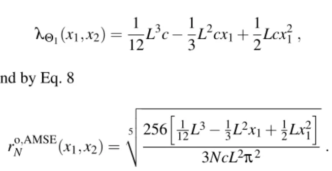
Fig. 1 shows, for c =700, the natural estimator for this type of random closed set as a function of the bandwidth, expressed in pixel (1 pixel=0.0029). To carry out the numerical experiments, we have studied the estimator at a fixed point (0.5, 0.5) of the compact windowW= [0,1]2.
For N = 10, Fig. 1a shows that the choice r =
rNo,AMSE provides a good estimation of the theoretical mean density; in fact, for this value of the bandwidth,
|bλΘν,N
1 (0.5,0.5)−λΘ1(0.5,0.5)| = 0.2973. For N = 100, Fig. 1b shows that the theoretical optimal value ofris still one of the best choices for the estimation of the mean density. One may notice that the estimation improves with respect to the caseN=10; in fact for
r=r100o,AMSEwe have|bλΘν,N
1 (0.5,0.5)−λΘ1(0.5,0.5)|= 0.0614. We conclude that the optimal bandwidth is one of the best choices for the estimation of the mean density, and asN→∞the estimation improves. Finally
we may observe that the natural estimator has good stability properties with respect to the choice of the bandwidth.
OPTIMAL BANDWIDTH FORbλµ,N
Θn
It is not difficult to see that
Bias(bλΘµ,N n (x)) =
P(x∈Θn⊕rN)
bd−nrd−n
−λΘn(x), (11)
Var(bλΘµ,N n (x)) =
λΘn(x) NrNd−nbd−n
+o
1
NrNd−n
. (12)
Therefore, it would be necessary to provide a Taylor series expansion ofBias(bλΘµ,N
n (x)), or equivalently of
0 10 20 30 40 50 60 70 80 90 0
10 20 30 40 50 60
r(pixel)
bλ
ν
,N Θ1
λ Θ
1
r
N o, AMSE
(a)
0 10 20 30 40 50 60
0 10 20 30 40 50 60
r(pixel)
bλ
ν
,N Θ1
λ Θ
1 r
N o, AMSE
(b)
Fig. 1. Comparison of the natural estimator and the theoretical value (λΘ1(0.5,0.5) = 13.30) at point (0.5,0.5) for an inhomogeneous Boolean model of segments with intensity f(x1,x2) =700x21. In (a) N = 10; for r10o,AMSE ≈ 77pixel(0.2973)
bλν,N
Θ1 (0.5,0.5) = 13.5973. In (b) N = 100; for ro100,AMSE≈49pixel(0.1425)bλΘν,N
1 (0.5,0.5) =13.2386.
A particular class of germ-grain models Θn for
which an explicit expression of P(x ∈ Θn⊕rN) is
available, is the class of Boolean models; in that case we get:
P(x∈Θn⊕rN) =
1−exp
n −
Z
K Z
x−Z(s)⊕rN
f(y,s)dyQ(ds)o. (13)
For numerical experiments of bλΘµ,N
n consider the
Boolean model of segments analyzed in Section
Optimal bandwidth forbλΘν,N n .
Since a general formula for the optimal bandwidth is not yet available in the literature, we will minimize the asymptotic approximation of the mean square error directly in this particular example. To this aim, a standard calculation of the integral in Eq. 13 leads to:
P(x∈Θ2⊕rN) =1−exp n
−cLrN
1
6L
2−2
3Lx1
+x21−1
6LπrN+ 1 2
4
3r
2
N+rNπx1
o
; (14)
then, by a Taylor series expansion of the exponential term in Eq. 14, we get that Bias(bλΘµ,N
2 (x)) =CBrN+
o(rN),where
CB(x1,x2):=−
1 12L
2 πc+1
4πx1cL
−1
4c
2L21
6L
2−2
3Lx1+x
2 1
2
,
and so AMSE(bλΘµ,N
2 (x)) =C
2
Br2N+λΘ1(x1,x2)/2NrN; thus it follows
roN,AMSE(x1,x2) = 3
s
λΘ1(x1,x2) 4NCB2(x1,x2).
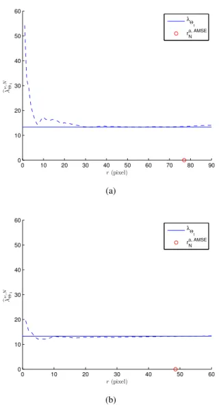
Fig. 2 shows the estimatorbλΘµ,N
n at point(0.5,0.5),as a
function of the bandwidthr(in pixel) for two different sample sizes (N=10,andN=100). In Fig. 2a, where the sample sizeN is equal to 10, we can observe that, near the optimal bandwidth,bλΘµ,N
1 provides a very good estimation of the mean density; in fact for the optimal value of r we have|bλΘµ,N
1 (0.5,0.5)−λΘ1(0.5,0.5)|= 1.8556. In Fig. 2b, where N = 100, the estimation improves; indeed |bλΘµ,N
1 (0.5,0.5)−λΘ1(0.5,0.5)| = 0.70,forrequal to the asymptotic optimal bandwidth. We can conclude that the optimal bandwidth leads to a good estimation of the mean density, which improves asNincreases.
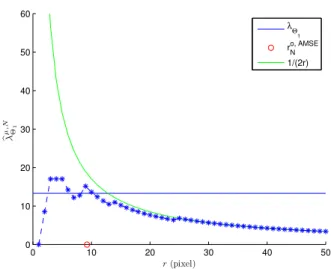
Finally observe that as r → +∞ the estimator
decreases as the function 21r (Fig. 3), in accordance with the definition of the estimator.
not yet available in literature.
0 10 20 30 40 50
0 10 20 30 40 50 60
r(pixel)
bλ
µ
,N
Θ
1
λ Θ
1
r N o, AMSE
(a)
0 10 20 30 40 50
0 10 20 30 40 50 60
r(pixel)
bλ
µ
,N
Θ1
λ Θ
1
r N o, AMSE
(b)
Fig. 2.Comparison of the “Minkowski content”- based estimator and the theoretical value (λΘ1(0.5,0.5) =
13.3) at point (0.5,0.5) for an inhomogeneous Boolean model of segments with intensity f(x1,x2) =
700x21. In (a) N =10; for r10o,AMSE ≈9pixel(0.0271)
b
λΘµ,N
1 (0.5,0.5) = 15.1556. In (b) N = 100; for ro100,AMSE≈4pixel(0.0126)bλΘµ,N
1 (0.5,0.5) =14.
PARTICULAR CASES
As a confirmation of the validity of our results, in this section we wish to present particular cases (for
n=0, and for stationaryΘn) which have already been
treated in literature.
0 10 20 30 40 50
0 10 20 30 40 50 60
r(pixel)
bλ
µ
,N
Θ1
λ Θ
1
rNo, AMSE 1/(2r)
Fig. 3.The “Minkowski content”-based estimator (for N = 10) at point (0.5,0.5) for an inhomogeneous Boolean model of segments with intensity f(x1,x2) =
700x21, compared with the function21r(in green).
RANDOM VARIABLES AND POINT
PROCESSES (n=0)
Let Θ0 ≡ X be a continuous random variable
with pdf fX (equivalently, with mean density λX =
fX). In order to apply the above results, X may be
considered as the trivial germ-grain process driven by the marked point processΦ={(X,s)}inRwith mark spaceK=Rd, consisting of one point (X) only, with grain Z(s) := s, and intensity measure Λ(d(y,s)) = f(y)dyδ0(s)ds, beingδ0the usual Dirac delta function
in 0. In this case the kernel estimatorbλXκ,N(x)defined in Eq. 4 reduces, as expected, to usual kernel density estimator for random variable well known in classical literature. Known results on the optimal bandwidth (Parzen, 1962; Silverman, 1986; Hardle, 1991, p. 59) follows now as particular case by Eq. 8 and Eq. 9. For a more detaild discussion, see Camerlenghiet al.(2014, Section 3.3.1). With regard to the natural estimator
bλν,N
X (x)and the “Minkowski content”-based estimator
bλµ,N
X (x), we notice that both estimators reduce, in this
case, to the usual histogram density estimator, also known in literature asnaive estimator,
bλXν,N(x) =bλXµ,N(x) = 1 N2rN
N
∑
i=1
1[x−rN,x+rN](Xi),
whereX1, . . . ,XN is an i.i.d. random sample forX.
As a more significant example of a random setΘ0
ΨinRd with intensity function fΨ. In Camerlenghiet
al.(2014) the following statement has been proven:
Proposition 4 Let {Ψi}i∈N be a sequence of point
processes in Rd, i.i.d. as Ψ, with intensity function
λΨ∈C2, and locally bounded second moment density
g, and let k be a kernel with compact support, continuous at 0. Then the kernel density estimator
b
λΨκ,N(x) = 1
NrdN
N
∑
i=1x
∑
j∈Ψik
x−xj
rN
(15)
of λΨ(x) is asymptotically unbiased and weakly
consistent forHd-a.e. x∈Rdif rNis such that
lim
N→∞
rN =0 and lim N→∞
NrNd =∞.
Moreover, the pointwise optimal bandwidth rNo,AMSE(x)
is given, forHd-a.e. x∈Rd, by
roN,AMSE(x) =
4+d
v u u u u u t
dλΨ(x) Z
Rd
k2(z)dz
4N
∑
|α|=21
α!D α
xλΨ(x) Z
Rd
k(z)zαdz2
,
while the global optimal bandwidth roN,,AMISEW is given, for any compact window W⊂Rd, by
roN,,AMISEW =
4+d
v u u u u u t
dE[Ψ(W)]
Z
Rd
k2(z)dz
4N
Z
W
∑
|α|=21
α!D α
yλΨ(x) Z
Rd
k(z)zαdz2dx
.
Note that by choosingk(z):= 1
bd1B1(0)(z) in Eq. 15,
with N=1, we reobtain the well known classic and widely used Berman-Diggle estimator (Diggle, 1985; Berman and Diggle, 1989; van Lieshout, 2012)
b
λΨκ,N(x) =Ψ(Br(x)) bdrd
.
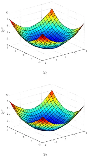
In order to show numerical results, let Ψ be a
Poisson point process in R2 with intensity function
λΨ(x1,x2) =x21+x22. We want to estimate the intensity
function ofΨin the compact windowW := [−2,2]2,
by means of bλΨκ,N(x) and bλΨν,N(x), for a sample size
N=1000.
Fig. 4a shows the first estimator, where we have adopted the kernel of Epanechnikov:
k(t) =
2
π(1−x 2
1−x22), if(x1,x2)∈B1(0)
0, otherwise
and the optimal bandwidth at each point of estimation, that is
rNo,AMSE(x1,x2) = 6
s
6(x21+x22)
Nπ ;
on the other hand, by Proposition 4, it is easy to see that the uniform optimal bandwidth at all points inW
is
rNo,,AMISEW = 6
r
64
Nπ .
We would like to compare the kernel estimation at (1.8,1.8), obtained by employing the optimal bandwidth at this point (bλΨκ,,No(1.8,1.8)), and the corresponding estimation generated by using the uniform optimal bandwidth in W (bλΨκ,,uN(1.8,1.8)).
At point (1.8,1.8) the theoretical value of the intensity function is λΨ(1.8,1.8) =6.48, the optimal
bandwidth isro1000,AMSE=0.4809 and the corresponding kernel estimation is bλΨκ,,No(1.8,1.8) = 6.4636 (|bλΨκ,,No(1.8,1.8)−λ(1.8,1.8)|=0.0164); instead the
uniform optimal bandwidth is ro1000,AMISE,W = 0.5226, and the corresponding estimation bλΨκ,,Nu(1.8,1.8) =
6.4350 (|bλΨκ,,Nu(1.8,1.8)−λ(1.8,1.8)|=0.045). Both
estimations are accurate, but the first one is better, since it employs the optimal bandwidth at the fixed point(1.8,1.8).
Fig. 4b shows the natural estimator in the compact window W, generated by employing the theoretical optimal bandwidth at each point in the compact window:
rNo,AMSE(x1,x2) = 6
s
2(x21+x22)
Nπ ;
as in the previous case, it is easy to obtain the uniform optimal bandwidth:
rNo,,AMISEW = 6
r
16 3Nπ .
As before, we will analyze the behavior of
b
λΨν,N(1.8,1.8), obtained by employing the optimal
6.4821 (|bλΨν,,No(1.8,1.8)−λ(1.8,1.8)|=0.0021); the
uniform optimal bandwidth isro1000,AMISE,W =0.3454, and the corresponding estimationbλΨν,,Nu(1.8,1.8) =6.5133 (|bλΨν,,Nu(1.8,1.8)−λ(1.8,1.8)|=0.0333). As before,
the first estimation is more accurate, since it employs the optimal bandwidth at the relevant point.
−2 −1
0 1
2
−2 −1 0 1 2 0 2 4 6 8 10
bλ
κ
,N
Ψ
(a)
−2 −1
0 1
2
−2 −1 0 1 2 0 2 4 6 8 10
bλ
ν
,N Ψ
(b)
Fig. 4. Estimators for the intensity function of a Poisson point process, for N=1000,for two different kernels. (a) showsbλΨκ,N(x1,x2), where k is the kernel of Epanechnikov and we have used the optimal bandwidth roN,AMSE(x1,x2)at each point. (b) shows the natural estimatorbλΨν,N(x1,x2); here we have used the optimal bandwidth rNo,AMSE(x)at each point.
THE CASE OF STATIONARYΘn
Let Θn be stationary; we assume here that, in
the point process representation, Φ = {(xi,si)}i∈N is an independent marking of the marginal process
{xi}i∈N, which is itself stationary, so thatΛ(d(x,s)) =
cdx Q(ds), i.e., f(x,s) ≡c, for any (x,s)∈Rd×K. Thus,λΘn(x)≡cE[H
n(Z)]for Hd-a.e.x∈
Rd, and the optimal bandwidthrNassociated with the proposed
estimators will be independent ofxas well.
Optimal bandwidth forbλΘκ,N
n andbλ
ν,N
Θn
We point out that in the stationary case a kernel type estimation would be irrelevant, since the intensity of the point process is constant; though we treat this case too in order to show the full compatibility of our approach with the standard one, in which we may just take global “means” in the observation window (see,
e.g., Beneˇs and Rataj (2004) and the next paragraphs for further details).
In (Camerlenghi et al., 2014) the following implications have been shown:
– (A1)⇒Bias(bλΘκ,N
n (x)) =0 for any bandwidthr>
0,and any sample sizeN;
– (A1) and (A3) ⇒ bλΘκ,N
n is strongly consistent for
Hd-a.e.x∈
Rd, asN→∞.
It is worth noting that whenever Θn is a Boolean
model such thatE[(Hn(Z))2]<∞, and the kernelkis
assumed to be continuous in the interior of its support, thenro,MSE= +∞(Camerlenghiet al., 2014).
The same conclusions hold for bλΘν,N
n too, by
choosing k(z) := 1
bd1B1(0)(z). This is in accordance
with both intuition and known results in literature for the optimal bandwidth of the kernel estimators of the intensity of homogeneous Poisson point processes. In particular, ifW is the observation window of any realization of a homogeneous Poisson point process
Ψ in Rd (and so N =1), and |W| its volume, being
bλΨν,1(x)(3)= 1
bdrdΨ(Br(0))for any x∈R
d, we reobtain
that the best unbiased estimator of the intensityλΨof
Ψis given by (takingro,MSE= +∞)bλΨ=Ψ(W)/|W|,
with|W| →∞.
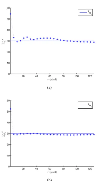
In order to carry out numerical experiments for
bλΘν,N
n in the stationary case, we have considered a
Boolean model of segments of the type [0,l]× {0}
with random length l ∼ U(0,L), where L = 0.2, in the compact window W = [0,1]2. Furthermore,
Fig. 5 shows the natural estimator at the fixed point
(0.5,0.5),for different values of the bandwidth r (in pixel). Since the optimal bandwidth is+∞,we expect that, as r grows to infinity, the estimation improves, which is confirmed: the estimator seems to stabilize after a certain value ofr. By comparing Fig. 5a, where
N=10, and b, whereN=100, the estimation improves as the sample size grows to infinity; in fact forN=100 the value after which the estimator stabilizes is less than the corresponding value forN=10.
20 40 60 80 100 120
0 10 20 30 40 50 60
r(pixel)
bλ
ν
,N Θ1
λ Θ
1
(a)
20 40 60 80 100 120
0 10 20 30 40 50 60
r(pixel)
bλ
ν
,N Θ1
λ Θ
1
(b)
Fig. 5. Comparison between the natural estimation and the theoretical value at the point (0.5,0.5) for a homogeneous Boolean model of segments with intensity f(x1,x2) =300. In (a) N =10; in (b) N =
100.The optimal bandwidth is+∞.
5.2.2 Optimal bandwidth forbλΘµ,N
n
We denote by Φi(A) the i-th total curvature
measure of any compact set A ⊂Rd with positive reach, as introduced in Federer (1959), for i =
0, . . . ,d−1.
Proposition 5 (Camerlenghi et al., 2014) Let Θn be
a Boolean model with intensity measure Λ(d(y,s)) = cdyQ(ds), satisfying Assumption (A1), and such that, for any s∈K,reachZ(s)>R,for some R>0. Let us assume also thatE[Φi(Z)]<∞for all i=0, . . . ,n−1. Then, the optimal bandwidth associated withbλΘµ,N
n is given by
roN,AMSE:=
3
s
cE[Hn(Z)]
N πcE[Φn−1(Z)]−2(cE[Hn(Z)])22
if d−n=1,
d−n+2
s
(d−n)bd−ncE[Hn(Z)]
2N cbd−n+1E[Φn−1(Z)] 2
if d−n>1, (16) independent of x∈Rd.
To understand further the behavior of bλΘµ,N
n in the
stationary case, consider the Boolean model of segments of the previous section. It is easy to calculate the optimal bandwidth, that is:
roN,AMSE= 3
s
cEL
N(cπ−2c2(
EL)2))2 . (17)
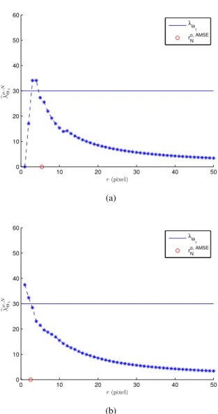
Fig. 6 shows bλΘµ,N
n (0.5,0.5) as a function of the
bandwidth r (in pixel). In Fig. 6a (N =10) observe that for r =roN,AMSE the estimation approaches very well the theoretical value of the mean density, even if N is low (|bλΘµ,10
1 (0.5,0.5)−λΘ1(0.5,0.5)|= 2.72). In Fig. 6b (N = 100) the best value of the estimation is achieved when r is equal to the theoretical optimal bandwidth, furthermore asNgrows the estimation improves; in fact, for r = r100o,AMSE,
|bλΘµ,100
1 (0.5,0.5)−λΘ1(0.5,0.5)| = 1.5833. We can conclude that the estimator is optimal for the choice
r = roN,AMSE and the estimation improves as the dimension of the sample size diverges to infinity. Finally, observe that as r → +∞, the estimator
0 10 20 30 40 50 0
10 20 30 40 50 60
bλ
µ
,N
Θ1
r(pixel)
λ Θ
1 r
N o, AMSE
(a)
0 10 20 30 40 50
0 10 20 30 40 50 60
bλ
µ
,N
Θ1
r(pixel)
λ Θ
1 r
N o, AMSE
(b)
Fig. 6.Comparison of the “Minkowski content”-based estimator and the theoretical value (λΘ1(0.5,0.5) =
30) at the point(0.5,0.5)for a homogeneous Boolean model of segments with intensity f(x1,x2) =300. In (a) we have chosen N=10;for r10o,AMSE≈5pixel(0.016),
we havebλΘµ,N
1 (0.5,0.5) =27.28. In (b) we have chosen N = 100, for r100o,AMSE ≈ 3pixel(0.0074), we have
b
λΘµ,N
1 (0.5,0.5) =28.4167.
CONCLUDING REMARKS
Based on the numerical simulations we may now offer here some comparison about the computational advantages / disadvantages of the estimators proposed by the authors in Villa (2014), and Camerlenghiet al.
(2014).
From a purely computationally point of view, it emerges the “Minkowski content”-estimator as
the most treatable, as one may easily realize by considering that for this estimator we just need to count relevant pixels of the random object (Eq. 6), while for the kernel estimator a, generally nontrivial, computation of integrals is required (Eq. 4). This is the main reason why we have reduced our numerical simulation to the sole point process case.
The natural estimator, which is a particular case of the kernel estimator, seems to be computationally easier to handle; further for point processes the choice of the kernel does not seem to be of much influence. The stationary case has been extensively studied in the literature. It is worth noticing that the optimal bandwidth for a generic kernel estimator is infinity, whenever Θn is a stationary Boolean model, in
accordance to well known results in the literature. In applied problems, an infinite optimal bandwidth is equivalent to the choice of an observation window as large as possible.
As far as the behaviour of the proposed estimators with respect to the choice of the bandwidth is concerned, we have in particular realized that the natural estimator results to be more stable; i.e., the “Minkowski content”-based estimators are quite sensitive to the choice of the bandwidth, while for kernel estimators it is only important that the bandwidth has the correct order of magnitude (Fig. 1-2).
For the time being we have not yet taken into account possible edge effects, which require further analysis.
ACKNOWLEDGMENTS
FC and EV are members of the Gruppo Nazionale per l’Analisi Matematica, la Probabilit`a e le loro Applicazioni (GNAMPA) of the Istituto Nazionale di Alta Matematica (INdAM); VC wishes to acknowledge the continued collaboration with ADAMSS, the Milan Interdisciplinary Centre for Advanced Applied Mathematical and Statistical Sciences.
It is our duty and a pleasure to acknowledge the anonymous referees for the accurate reading of the paper, and their valuable comments and suggestions which lead to an effective improvement of the presentation of our results.
REFERENCES
Ambrosio L, Fusco N, Pallara D (2000). Functions of bounded variation and free discontinuity problems. Oxford: Clarendon Press.
Baddeley A, Barany I, Schneider R, Weil W (2007). Stochastic geometry. Lect Not Math 1982. Berlin: Springer.
Beneˇs V, Rataj J (2004). Stochastic geometry: selected topics. Dordrecht: Kluwer.
Berman M, Diggle P (1989). Estimating weighted integrals of the second-order intensity of a spatial point process. J Roy Statist Soc B 51:81–92.
Camerlenghi F, Capasso V, Villa E (2014). On the estimation of the mean density of random closed sets. J Multivariate Anal 125:65–88.
Capasso V, Villa E (2006). On the continuity and absolute continuity of random closed sets. Stoch An Appl 24:381–97.
Capasso V, Villa E (2007). On mean densities of inhomogeneous geometric processes arising in material science and medicine. Image Anal Stereol 26:23–36. Capasso V, Villa E (2008). On the geometric densities of
random closed sets. Stoch Anal Appl 26:784–808. Daley DJ, Vere-Jones D (1988). An introduction to the
theory of point processes. Probab Appl 2003. New York: Springer.
David G, Semmes S (1997). Fractured fractals and broken dreams-self-similar geometry through metric and measure. London: Oxford Univ Press.
Deheuvels P, Mason DM (2004). General asymptotic confidence bands based on kernel-type function estimators. Stat Inference Stoch Process 7:225–77. Diggle PJ (1985). A kernel method for smoothing point
process data. Appl Statist 34:138–47.
Falconer KJ (1985). , The geometry of fractal sets. Cambridge: Cambridge University Press.
Falconer KJ (2004). One-sided multifractal analysis and points of non-differentiability of devil’s staircases. Math Proc Cambridge Philos Soc 136:167–74.
Federer H (1959). Curvature measures. Trans Amer Math Soc 93:418–91.
Federer H (1969). Geometric measure theory. Berlin: Spriger.
H¨ardle W (1991). Smoothing techniques with implementation in S. New York: Springer-Verlag. Hug D, Last G, Weil W (2002). A survey on contact
distributions. In: Mecke KR, Stoyan D, Eds. Morphology of condensed matter. Physics and geometry of spatially complex systems. Lect Not Phys 600:317–57. Berlin: Springer.
Hug D, Last G, Weil W (2004). A local Steiner-type formula for general closed sets and applications. Math Z
246:237–72.
Karr AF (1986). Point processes and their statistical inference. New York: Marcel Dekker.
Matheron G (1975). Random sets and integral geometry. New York: John Wiley & Sons.
Parzen E (1962). On the estimation of a probability density function and the mode. Ann Math Statist 33:1065–76. Rosenblatt M (1956). Remarks on some nonparametric
estimates of a density function. Ann Math Statist 27:832–7.
Schucany WR (1989). Locally optimal window widths for kernel density estimation with large samples. Statist Probab Lett 7:401–5.
Silverman BW (1986). Density estimation for statistics and data analysis. London: Chapman & Hall.
Stoyan D, Kendall WS, Mecke J (1995). Stochastic geometry and its application. New York: John Wiley & Sons.
van Lieshout MNM (2012). On estimation of the intensity function of a point process. Meth Comput Appl Probab 14:567-78.
Villa E (2010). Mean densities and spherical contact distribution function of inhomogeneous Boolean models. Stoch An Appl 28:480–504.
Villa E (2014) On the local approximation of mean densities of random closed sets. Bernoulli 20:1–27
Wertz W (1978). Statistical density estimation: a survey. Angewandte Statistik und Okonometrie [Applied¨ statistics and econometrics] 13 G¨ottingen: Vandenhoeck & Ruprecht.
APPENDIX
To fix the notation, α := (α1, ...,αd) will be a
multi-index ofNd0; we will denote
|α|:=α1+· · ·+αd
α! :=α1!· · ·αd!
yα:=yα1 1 · · ·y
αd
d
Dα
y f(y,s):=
∂|α|f(y,s) ∂yα11· · ·∂yαdd
;
furthermore, for alls∈K,we will denote
D(α)(s):=disc(Dα
y f(y,s)), D(s):=disc(f(·,s)).
Furthermore, we list here the assumptions onΦwhich
have been adopted in the text.
(A1) for any (y,s)∈Rd×K, y+Z(s) is a countably
Hn-rectifiable and compact subset of
R
KHn(Ξ(s))Q(ds)<∞and
Hn
(Ξ(s)∩Br(x))≥γrn ∀x∈Z(s),∀r∈(0,1)
(18) for someγ>0 independent ofs;
(A1)as (A1), replacing (18) with
γrn≤Hn(
Ξ(s)∩Br(x))≤eγrn ∀x∈Z(s),r∈(0,1)
for someγ,γe>0 independent ofs;
(A2) for anys∈K,Hn(disc(f(·,s))) =0 and f(·,s)is locally bounded such that for any compactK⊂Rd
sup
x∈K⊕diam(Z(s))
f(x,s)≤ξeK(s)
for someξeK(s)with
Z
KH
n
(Ξ(s))ξeK(s)Q(ds)<∞;
(A2bis) for any s ∈ K, Hn(D(α)(s)) = 0 and Dα
y f(y,s) is locally bounded such that, for any
compactC⊂Rd,
sup
y∈C⊕diamZ(s)
|Dα
y f(y,s)| ≤ξe
(α)
C (s)
for someξeC(α)(s)with
Z
KH
n
(Ξ(s))ξeC(α)(s)Q(ds)<∞;
(A3) for any(s,y,t)∈K×Rd×K,Hn(disc(g(·,s,y,t))) = 0 and g(·,s,y,t) is locally bounded such that for any compactK⊂Rd anda∈Rd,
1(a−Z(t))⊕1(y) sup
x∈K⊕diam(Z(s))
g(x,s,y,t)≤ξa,K(s,y,t)
for someξa,K(s,y,t)with
Z
Rd×K2H
n
(Ξ(s))ξa,K(s,y,t)dyQ[2](ds,dt)<∞.
(19)
(A3)for anys,t∈K,g(·,s,·,t)is locally bounded such that, for anyC,C⊂Rd compact sets:
sup
y∈C⊕diamZ(t)
sup
x∈C⊕diamZ(s)
g(x,s,y,t)≤ξC,C(s,t)
for someξC,C(s,t)with
Z
K2H
n(
Ξ(s))Hn(
Ξ(t))ξC,C(s,t)Q[2](ds,dt)<∞.
(20)
For a discussion on the above assumptions and on how they simplify in certain particular cases, for instance whenever Θn is a Boolean model (i.e., Φ is