Can Interviewer Observations of the Interview Predict Future Response?

Can Interviewer Observations of the

Interview Predict Future Response?

Ian Plewis

_{, Lisa Calderwood}

_{& Tarek Mostafa}

1

University of Manchester

2

Centre for Longitudinal Studies, UCL Institute of Education

Abstract

Interviewers made four observations related to future participation, respondent coopera-tion, enjoyment and whether the respondent found the questions difficult, for a large sample of face-to-face interviews at wave four of the UK Millennium Cohort Study (MCS). The focus of the paper is on predicting response behavior in the subsequent wave of MCS, four years later. The two most predictive observations are whether the respondent is likely to participate in the next wave and whether they enjoyed the interview. Not only do these predict non-response at the next wave, they do so after controlling for other explanatory variables from earlier waves in a response propensity model. Consequently, these two in-terviewer observations improve discrimination between respondents and non-respondents at wave five as estimated by Gini coefficients generated by a Receiver Operating Charac-teristic curve analysis. The predicted probabilities of responding at wave five are also used to estimate R-indicators, particularly to address the question of whether, hypothetically, conversion of ‘frail’ respondents would lead to improved representativity and reduced bias in longitudinal estimates of interest. The evidence from the indicators and partial R-indicators suggests that successful conversions could achieve those aims although the cost of so doing might outweigh the benefits.

Keywords: Millennium Cohort Study; non-response; representativity; response propen-sity models; ROC curve.

Acknowledgements

The interviewer observations reported in this paper were collected as part of a re-search project entitled ‘Predicting and Preventing Non-Response in Cohort Studies’ (Ref: RES-175-25-0010). This project was funded by the UK’s Economic and Social Research Council (ESRC) as part of their Survey Design and Measurement Initia-tive (SDMI). The UK Millennium Cohort Study (MCS) is funded by the ESRC and a consortium of UK government departments. The National Centre for Social Research (NatCen) carried out the data collection in Great Britain for the fourth wave of MCS; we would like to thank their research and operational staff who were responsible for the implementation of the interviewer observations. Ipsos MORI carried out the data collection for the fifth wave of MCS. We would also like to thank Rebecca Taylor for her contributions to this research, and the referees and Editor for helpful comments on an earlier version of this manuscript.

Direct correspondence to

Ian Plewis, Social Statistics, Humanities Bridgeford Street, Manchester M13 9PL, UK

E-mail: [email protected]

1 Introduction

An important goal for managers of longitudinal surveys is to maintain response over time so that researchers can have some confidence in their inferences about change. Various strategies are used: incentives (both to respondents and interview-ers), reissuing refusals etc. Many of these issues are discussed in Lynn (2009). Another possibility is to direct extra resources at those respondents with a higher risk of not responding, a risk that is often estimated from response propensity mod-els that include predictors from previous waves. Often, however, predictions of future non-response are imprecise so that targeted interventions might not be cost-effective (Plewis & Shlomo, 2013). Our paper focuses on interviewer observations of a face-to-face interview. We investigate the characteristics of these observations and whether they can improve the prediction of non-response at the subsequent wave of data collection, both on their own and, more importantly, over and above the variables that are commonly included in response propensity models. We then go on to consider the implications for the longitudinal sample of a hypothetical situation in which respondents deemed to be at high risk of not responding at the subsequent wave are retained in the sample.

attention from researchers. Eckman et al. (2013) provide a summary although none of the studies reviewed by them are in peer-reviewed journals. The context for the empirical investigation in Eckman et al. (and also in Sinibaldi & Eckman, 2015) is a German cross-sectional telephone survey. Essentially, interviewers were asked to rate the probability that the case would complete the interview at a later contact attempt (conditional on them not doing the interview at that contact). The authors do find that the higher the probability rating the more likely a subsequent interview, although the association appears to be non-linear and not to be strong. Sinibaldi & Eckman (2015) extend the analysis by showing that discrimination between com-pletion and non-comcom-pletion is slightly improved when the interviewer ratings are added to a response propensity model that already includes other ‘call’ variables to predict outcome. They also consider how these ratings might be used in a hypo-thetical adaptive design to improve cooperation rates. Neither Eckman et al. nor Sinibaldi & Eckman address the question of whether these interviewer variables will lead to a reduction of non-response bias in outcomes of interest.

Few studies have used interviewer observations in a longitudinal context. We have previously shown (Plewis et al., 2012) that interviewer observations of neigh-borhood at wave two in the study used in this paper - the ongoing UK birth cohort study known as the Millennium Cohort Study (MCS) - predict response one wave later. West et al. (2014) collected interviewer ratings of income (in terciles) and whether the respondent was receiving unemployment benefit to supplement survey measures of these variables. They found that, in terms of non-response adjustment, these observations do not have any additional effect on their chosen cross-sectional estimates having incorporated prior survey measures of economic variables in their response propensity model. Uhrig (2008), using data from waves one to 14 of the British Household Panel Survey, shows that an interviewer rating at the end of the interview of respondent cooperativeness during the interview (a five point scale) predicts later response, after controlling for other variables in a discrete time haz-ard model with attrition as an absorbing state. He modeled non-contact (a category that includes not located) and refusal separately and found that the model estimates increase monotonically across the five point scale and are statistically significant for both response categories although they are stronger for refusal. None of this cited work considers how interviewer observations might be used in adaptive longi-tudinal designs to maintain response over time.

The paper is organized as follows. Section 2 describes the data used for our empirical investigations and presents some basic descriptive statistics. Section 3 sets out our research questions in their statistical modeling context. Section 4 pres-ents the results from our models. Section 5 concludes with some reflections on our results and their implications for future longitudinal investigations.

2 Data

The data for this investigation come from a methodological study incorporated into wave four of the UK Millennium Cohort Study (MCS). Wave one of MCS includes children from 18,552 families born over a 12-month period during the years 2000 and 2001, and living in selected UK electoral wards at age nine months. The initial response rate was 72%. Areas with high proportions of Black and Asian families, disadvantaged areas and the three smaller UK countries are all over-represented in the sample which is disproportionately stratified and clustered as described in Plewis (2007). The first five waves took place when the cohort members were (approximately) nine months, 3, 5, 7 and 11 years old (in 2012). The data collec-tion for the study takes place in the home and involves face-to-face interviews with multiple informants in each family. Interviews have been sought with up to two co-resident parents at every wave. At wave five, 31% of the target sample – which excludes child deaths and emigrants – were unproductive in the sense of not provid-ing any data (Mostafa, 2014).

During wave four of MCS, interviewers were asked to rate (using five point scales) some aspects of the interview after it was completed: whether participation was likely at the next sweep (i.e. wave); and observations of (i) cooperation during the interview and (ii) whether the respondent had enjoyed the interview. In addi-tion, interviewers were asked to assess whether the respondents had found answer-ing any of the questions difficult or uncomfortable. The motivation for the first three of these observations is clear in terms of the previously cited literature and their face validity; the final observation was included because it was expected to tap an aspect of the interview more closely related to the actual interaction between interviewer and respondents. Appendix A gives the wording for the interviewers when making the observations.

obser-vation where responding partners were perceived to have found the questions, if anything, less difficult and uncomfortable. Agreement between the observations for main respondents and their partners (aggregated over interviewers) was moderate: the kappa estimates (weighted to reflect the extent of disagreement) are 0.50 (s.e. = 0.01; n = 8739) for enjoyment; 0.43 (0.01; 8741) for cooperation and 0.40 (0.01; 8741) for the binary ‘questions difficult’. We do not know whether decisions about participating in MCS are made independently or jointly within households. In this paper, we concentrate on predicting non-response at the household level, treating as responding any household that provides at least some data. Consequently, we combine the respondent and partner assessments to generate a single variable for modeling response propensities and we do this by taking the more negative rating for each observation if two observations were made. This does assume that deci-sions are more likely to be made jointly by the main respondent and her/his partner and has the advantage, in the modeling, of having variables which are less skewed to the positive end of the scale and show more variation.

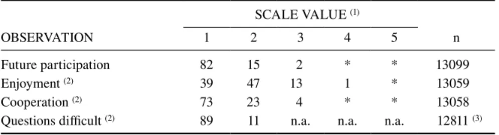
Table 1 gives the descriptive results for the four interviewer observations. It shows that all four are skewed towards the positive ends of the scales although less so for ‘enjoyment’. The participation, enjoyment and cooperation questions all correlate moderately with each other but there is no correlation between ‘questions difficult’ and the other three variables which suggests that this observation is, as anticipated, tapping a different dimension of the interview. As our main interest is in analyzing response at wave five, we treat the issued sample at wave five that was productive at wave four (n = 13108) as our base sample. Overall non-response is 11%. Most of the non-response comes from cases who refuse (n = 1102; 8% of all cases); not located (i.e. untraced) is 1.1% (n = 155) and non-contact conditional on Table 1 Percentage distributions of interviewer observations

OBSERVATION

SCALE VALUE (1)

1 2 3 4 5 n

Future participation 82 15 2 * * 13099

Enjoyment (2) _{39 47 13 1 * 13059}

Cooperation (2) _{73 23 4 * * 13058}

Questions difficult (2) _{89 11 n.a. n.a. n.a. 12811} (3)

Notes:

(1) _{Scale value ‘1’ represents the positive end of the scale, ‘3’ is neutral (‘difficult to say’ or} ‘fair’), ‘5’ the most negative. *: < 0.5%.

(2) _{Main respondent and partner observations were combined in such a way that the more} negative rating was dominant. When there was no partner interview, the main respon-dent rating was used (and vice-versa).

being traced is 1.7% (n = 218). There was very little non-response – less than 1% - for the interviewer observations as indicated by the final column of Table 1. The percentages in Table 1 allow for the sample design (disproportionate stratification and clustering); sample sizes (n) are the actual number of observations.

The child’s ethnic group and the highest level of educational qualifications achieved by the main respondent are key socio-demographic variables in MCS in that they are associated with many of the economic, social, health and cognitive outcomes of interest. We therefore assess whether these key variables are associated with the interviewer observations. We find that, when these variables are explana-tory variables in ordered (i.e. proportional odds) and binary logistic regressions, they both predict all the interviewer observations. Interviewers expect participation at the next wave to be less likely among the mixed, Pakistani and Bangladeshi, and Black Caribbean and African ethnic groups than for whites, Indians and others; p < 0.001 on a Wald test. The results for enjoyment, cooperation and ‘questions dif-ficult’ are similar although not identical. Pakistani and Bangladeshi, Black Carib-bean and African, and ‘other’ ethnic groups are assessed to have enjoyed the inter-view less and to have been less cooperative whereas all the minority ethnic groups apart from the mixed group were more likely to have found the questions difficult (Wald tests all p < 0.001). Mothers with lower qualifications were more likely to be assessed at the more negative points on all four scales (Wald tests all p < 0.001).

3 Methods and Models

We fit statistical models to answer three questions. The first is whether interviewer observations at wave t predict overall non-response, and categories of non-response, at wave t+1, both separately and when put together in a single model. Moreover, do these observations predict response at wave t+1 conditional on the inclusion in a response propensity model of established explanatory variables from previous waves? The full response propensity model is:

( )

0 1

K L

i k ki l li

k l

logit ρ β x γ z

= =

=

∑

∑

where ρi =E(ri) is the probability of responding for unit i (i = 1..n); ri =0 for

non-response and 1 for response;

x

waves and listed in Appendix B (x0 = 1); zlare the interviewer observations. ML

estimates of βk (=bk) and γl(= cl) are easily obtained, leading to predicted

0 1 / 0 1

ˆ 1

K L K L

k ki l li k ki l li

k l k l

b x c z b x c z

i e e

ρ = = = =

+  + 

 

= _ + _

 

 

∑

∑

∑

∑

The second question is: how much improvement is provided by the interviewer observations in terms of discriminating between respondents and non-respondents at wave t+1, as measured by analyses using Receiver Operating Characteristic (ROC) curves? Our approach to this question is based on estimating the predicted probabilities (ρˆ_i) of responding at wave five from the response propensity models without and with interviewer assessments. It is set out in detail in Plewis et al. (2012). We present just the essentials of this method here.

Plewis et al. (2012) show how ROC curves can be used to discriminate between, or to predict whether cases are more likely to be respondents or non-respondents. In brief, if + (i.e. 1− >ρˆ_i c)refers to a prediction of non-response where c is any threshold from the distribution of ρˆ_ithen the ROC is the plot of P(+| r = 0) against P(+| r = 1) where r is the observed response category, i.e. a plot of the true positive fraction (TPF) against the false positive fraction (FPF) for all c.

The area enclosed by the ROC curve and the x-axis, known as the AUC (area under the curve), is of particular interest and this can vary from 1 (when the model for predicting response perfectly discriminates between respondents and non-respondents) down to 0.5, the area below the diagonal (when there is no discrimina-tion between the two categories). The AUC can be interpreted as the probability of assigning a pair of cases, one respondent and one non-respondent, to their correct categories, bearing in mind that guessing would correspond to a probability of 0.5. A linear transformation of AUC (= 2*AUC – 1), often referred to as a Gini coef-ficient, is commonly used as a more natural measure than AUC because it varies from 0 to 1.

Plewis et al. (2012) also use a method developed by Copas (1999) known as a logit rank plot. For response propensity models based on logistic regression, this is just a plot of the linear predictor from the model against the logistic transformation of the proportional rank of the propensity scores. Copas argues that this approach is more sensitive to changes in the response propensity model than an approach based on ROC curves.

the observed sample deviates from the target sample in terms of likely bias. It is estimated by:

1 2ˆ ˆ

Rρ= − Sρ (3)

where ρ is the probability of responding, estimated from the response propensity model as in (2), and Sˆρ is the standard deviation of these estimated probabilities.

Standard errors of Rˆρ for clustered and weighted samples are discussed by Plewis

& Shlomo (2013). It is important to note that the estimate of R is conditional on the specification of the response propensity model.

We also use unconditional partial R-indicators (R_p(u)) for the third question. Unconditional partial R-indicators for a variable Z having categories j, j = 1..J show how representativeness varies across this variable and thus provides an indication of where the sample is particularly deficient (or satisfactory). Conditional on the response propensity model, the variable level unconditional partial R-indicator is estimated as:

( ) 2

1

ˆ_{p u} [J _j(ˆ_j ) ]ˆ

j

R p ρ ρ

=

=

∑

where pj is the estimated proportion in category j, ρˆj is the estimated (mean)

response rate in category j and ρˆ is the estimated overall response rate. A reduc-tion in Rˆp u_{( )} indicates an improvement in representativeness with respect to that

variable.

At the category level, Z = j, the unconditional partial indicator is estimated as:

( ),

ˆ_{p u j j}

R = p (ρ ρˆj−ˆ)

Note that Rˆp u j_{( )}, can be negative (under-representation) or positive

(over-represen-tation).

4 Results

Here, we give the results for the three questions posed in the previous section.

4.1 Are interviewer observations predictive?

in Table 2. The estimates increase monotonically except for the final categories which have few observations (see Table 1).

Table 2 Estimates from logistic regressions for each observation

OBSERVATION

Estimate (s.e.)

2 3 4 5 n

Future participation -1.02 (0.089) -1.71 (0.16) -2.52 (0.37) -1.43 (0.42) 13099 Enjoyment -0.44 (0.084) -0.94 (0.11) -1.59 (0.22) -1.27 (0.35) 13059 Cooperation -0.56 (0.073) -1.14 (0.13) -1.35 (0.35) -1.37 (0.53) 13058 Questions difficult -0.52 (0.094) n.a. n.a. n.a. 12811

Notes

1. The reference category is the most positive rating.

2. The models are fitted using the svy procedures in STATA and so allow for the sample design.

When wave five non-response is broken down into not located, not contacted and refusal, we find that ‘future participation’ and ‘questions difficult’ predict all three non-response categories but ‘enjoyment’ and ‘cooperation’ only predict refusal (conditional on being contacted) and non-contact (conditional on being located). The fact that the observation of likely future participation predicts whether or not someone is located at the next wave suggests that interviewers pick up clues during or after the interview about family plans to move, making it difficult to interpret this association. Because non-contacts are sometimes regarded as disguised refus-als (Blom, 2014), and because the relations between the observations and these two categories are similar, we combine these two categories and omit the not located cases from the rest of the analyses presented here. Hence, we work with a new binary variable r*_{: refused or not contacted (r}* _{= 0) and responded (or productive)} (r* _{= 1).}

When all four interviewer observations are entered together into a single model, we find that ‘future participation’ and ‘enjoyment’ conditionally predict r* but ‘cooperation’ and ‘questions difficult’ do not. The estimates and p-values from Wald tests from the logistic regression model are: (-0.84, -1.39, -2.25, -1.44), p<0.001 (‘future participation’); (-0.21, -0.41, -0.56, -0.28), p<0.03 (‘enjoyment’); (-0.013, -0.10, -0.065, -0.40), p>0.9 (‘cooperation’); 0.16, p >0.15 (‘questions difficult’). Con-sequently, we focus on ‘future participation’ and ‘enjoyment’ from now on.

be achieved with the usual response propensity models in longitudinal research. The extent of that improvement is now addressed.

Table 3 Estimates for the two interviewer observations in the full response propensity model

OBSERVATION

Estimate (s.e.)

2 3 4 5 n

Future participation -0.58 (0.11) -0.94 (0.19) -1.97 (0.41) -1.45 (0.44) 12880 Enjoyment -0.28 (0.090) -0.50 (0.13) -0.82 (0.25) 0.39 (0.41)

4.2 Is discrimination improved?

The two interviewer observations increase the AUC from 0.68 (s.e. = 0.0079) to 0.70 (s.e. = 0.0076). This difference is greater than expected by chance ( 2

1 23.8, 0.001;p n 12880

χ = < = ) from the roccomp procedure in STATA. This means the Gini coefficient increases from 0.36 to 0.41. The slopes of the logit rank plots tell a similar story: an increase from 0.38 (0.011) to 0.43 (0.013).

These results indicate that the two more predictive interviewer observations do improve the prediction of non-response. Whether this model would also be better for adjusting for non-response using non-response weights or imputation methods, does, however, require that the observations are correlated with outcome variables of interest, more particularly changes in these variables, as well as with response behavior. This is also one of the requirements for targeting interventions at poten-tial non-respondents although maintaining the sample over time does also have benefits in terms of precision. We do not address this question directly here but return to it in the concluding section.

4.3 Implications for representativity?

Given that the interviewer observations at wave t are predictive of response at wave t+1 and taking advantage of the fact that they can be made available to survey managers soon after fieldwork for wave t has been completed, another way of using them is to define a set of what we might call ‘frail’ respondents who have a low rat-ing (i.e. 3 or below) on at least one of the two most predictive observations. In prin-ciple, it would be possible to direct extra resources (such as using more experienced interviewers or financial incentives) at these ‘frail’ respondents with the intention of preventing them from becoming non-respondents at the next wave.

There were 352 frail respondents as defined above who were indeed non-respondents at wave five. We use the response propensity model without the inter-viewer observations to estimate R. Were our interventions to convert all these non-respondents into non-respondents at wave five successful, then the estimate of R would increase from 0.86 (the estimate given above) to 0.91. Of course, no interventions to prevent non-response will have a 100% success rate. Moreover, any intervention will also be directed at ‘frail’ respondents who did, in the event, respond at wave five: there were 1838 of these in our example so the targets of the intervention would form perhaps only a sixth of the intervention group. We could reduce this ‘deadweight’ problem by having a stricter criterion such as respondents receiving a rating in just the two lowest categories for at least one of the observations. This would reduce the size of the intervention group to 290 of which 63 (22%) actually failed to respond at wave five. The effect on representativity is then smaller (0.87 compared with 0.86). Nevertheless, this approach does demonstrate the possibili-ties of combining interviewer observations with targeted interventions in terms of maintaining the sample over time and reducing the overall bias in the sample. We can provide at least some evidence about whether non-response bias in outcome variables of interest will be reduced by estimating unconditional partial R-indica-tors for the two key variables introduced earlier – ethnic group and qualifications.

We find that the unconditional partial R-indicator for ethnic group would decline slightly - from 0.018 to 0.014 - if frail respondents were maintained in the sample (using the less strict criterion of frailty). The decline inRˆp u_{( )}for

qualifica-tions is more marked: 0.031 to 0.021. The estimates of Rˆ_{p u j( ),} show that under-representation of the mixed and black groups, and the over-under-representation of the highly qualified groups, would both be reduced. This suggests that keeping the frail respondents in the sample might lead to a reduction in bias in estimates of interest.

5 Discussion

34 interviewers randomly assigned to cases in their telephone survey, about nine per cent of the variation in their one rating could be attributed to interviewers. About 400 interviewers were used in wave four of MCS and, as is common in such large face-to-face longitudinal surveys, they were not randomly allocated to cases. Consequently, we have no estimate of the interviewer effect for our observations although we can be sure that interviewers will have observed ‘similar’ interviews in different ways. It is probable that the variation between interviewers, if estimable, would have had a small effect on the estimates in our models, the most likely effect being to increase their standard errors. If the proportion of overall variation allo-cated to interviewers for our observations were similar to the estimate found by Eckman et al. (2013), and given a mean interviewer workload of about 30 cases, then we might expect to see a doubling of the standard errors. Most of our results are robust to such a reduction in the estimates’ precision. Further investigation of this topic is, however, warranted.

This study used four interviewer observations; the only closely related study (Uhrig, 2008) used just one – a measure of cooperativeness – which did predict future response one year later. The evidence presented here suggests that an obser-vation of cooperativeness is not as predictive as the obserobser-vations of future par-ticipation and enjoyment. Hence, it is these two variables that researchers might consider giving priority to if they are in a position to collect such paradata in order to improve predictions via a better response propensity model. The ‘questions dif-ficult’ variable does appear to be tapping another aspect of the interaction between interviewer and respondent but is not as good a predictor of future response as the others.

propensity to respond and not with the outcome – for the model to be identified and interviewer observations measuring aspects of the interview itself could be useful instruments in that context.

We have focused here on the relation between interviewer observations and later non-response. It is, however, possible that observations of this kind could be used in other ways. In particular, they might be useful as accuracy indicators (Da Silva & Skinner, 2013) in order to get a handle on the extent of measurement error in the responses. It is plausible that the ‘questions difficult’ observation would be the most useful for this purpose. This is also a topic worthy of further investigation.

It remains an open question as to whether the benefits of collecting these kinds of interviewer observations outweigh their costs. Interviewers do have to be paid to complete these observations, perhaps only a small amount per interview, but a considerable sum in the aggregate. Hence, if field work budgets are fixed, some questions might, for example, have to be dropped from the questionnaire to accom-modate them. The assessment of the benefits hinges on two related questions. First, would the incorporation of interviewer observations into a response propensity model lead to sufficiently improved non-response weights and imputations (i.e. greater bias reduction and more precision)? Second, would the retention of frail respondents in the sample as a result of a targeted intervention reduce bias and increase precision. This paper, along with Sinibaldi & Eckman (2015), does provide grounds for supposing that the answer to the first question could be positive. Both papers found, for example, similar increases (0.03 to 0.05) in the estimated Gini coefficients as a result of including observations in a response propensity model. The contexts for the two studies were, however, very different: a cross-sectional telephone survey with a low response rate and with predictions limited to a window of at most a few weeks, compared with an ongoing longitudinal study with high wave on wave response rates and predictions of response behavior four years later. An affirmative answer to the second question does depend on designing a success-ful intervention and being prepared to carry the cost of directing this intervention to a substantial ‘deadweight’ group of frail respondents who would have responded anyway.

References

Blom, A. G. (2014). Setting priorities: Spurious differences in response rates. International Journal of Public Opinion Research, 26(2), 245-255. doi:10.1093/ijpor/edt023

Copas, J. (1999). The effectiveness of risk scores: The logit rank plot. Applied Statistics, 48(2), 165-183. doi:10.1111/1467-9876.00147

Da Silva, D. N., & Skinner, C. (2013). The use of accuracy indicators to correct for survey measurement error. Applied Statistics, 63(2), 303-319. doi:10.1111/rssc.12022

Eckman, S., Sinibaldi, J., & Möntmann-Hertz, A. (2013). Can interviewers effectively rate the likelihood of cases to cooperate? Public Opinion Quarterly, 77(2), 561-573. doi:10.1093/poq/nft012

Kreuter, F. (Ed.) (2013). Improving surveys with paradata: Analytic uses of process infor-mation. Chichester: John Wiley & Sons.

Kreuter, F., Olson, K., Wagner, J., Yan, T., Ezzati-Rice, T. M., Casas-Cordero, C., Lemay, M., Peytchev, A., Groves, R. M., & Raghunathan, T. E. (2010). Using proxy measures and other correlates of survey outcomes to adjust for non-response: Examples from multiple surveys. Journal of the Royal Statistical Society: Series A, 173(2), 389-407. Lynn. P. (Ed.) (2009). Methodology of longitudinal surveys. Chichester: John Wiley & Sons. Mostafa, T. (2014). Millennium Cohort Study: Technical Report on Response in Sweep 5.

Centre for Longitudinal Studies: London

Plewis, I. (2007). The Millennium Cohort Study: Technical Report on Sampling (4th_{. Ed.).}

Centre for Longitudinal Studies: London.

Plewis, I., Ketende, S. C., Joshi, H., & Hughes, G. (2008). The contribution of residential mobility to sample loss in a birth cohort study: Evidence from the first two waves of the Millennium Cohort Study. Journal of Official Statistics, 24(3), 365-385.

Plewis, I., Ketende, S., & Calderwood, L. (2012). Assessing the accuracy of response pro-pensity models in longitudinal studies. Survey Methodology, 38(2), 167-171.

Plewis, I., & Shlomo, N. (2013). Statistical guidance on optimal strategies to reduce non-response in longitudinal studies. CCSR Working Paper 2013-03. Manchester: CCSR. Schouten, B., Cobben, F., & Bethlehem, J. (2009). Indicators of the representativeness of

survey response. Survey Methodology, 35(1), 101-113.

Sinibaldi, J., & Eckman, S. (2015). Using call-level interviewer observations to improve response propensity models. Public Opinion Quarterly, 79(4), 976-993. doi:10.1093/ poq/nfv035

Uhrig, N. (2008). The nature and causes of attrition in the British Household Panel Survey.

Working Paper 2008-05. ISER: Essex.

Appendix A

Interviewer observations

This is how the four interviewer observations were worded:

1. In your opinion, how likely is it that anyone will take part in the next sweep of Child of the New Century: (1) very likely; (2) fairly likely; (3) difficult to say; (4) fairly unlikely; (5) very unlikely.

[Child of the New Century is a label used by field staff to describe the Millen-nium Cohort Study.]

2. In general, how would you rate the co-operation of {main respondent (name)/ partner respondent (name)} during the interview: (1) very good; (2) good; (3) fair; (4) poor; (5) very poor.

3. On the whole, did {main respondent (name)/partner respondent (name)} seem to enjoy the interview: (1) enjoyed a great deal; (2) enjoyed to some extent; (3) difficult to say; (4) did not enjoy some of it; (5) did not enjoy at all.

Appendix B

Model estimates from response propensity model (in 4.1)

VARIABLE ESTIMATE (s.e.) 95% CI

Child sex (ref: boy) -0.21 (0.072) (-0.35, -0.069)

Main respondent’s age

(ref: 20-29) _30-39<20 -0.18 (0.10)_{0.36 (0.10)} (-0.37, -0.018) _{(0.15, 0.56)} 40+ 0.60 (0.44) (-0.28, 1.47) Ethnic group (ref: white) Mixed -0.15 (0.19) (-0.53, 0.23) Indian 0.22 (0.24) (-0.25, 0.69) Pakistani/Bangladeshi 0.88 (0.20) (0.48, 1.28) Black -0.48 (0.18) (-0.84, -0.13) Other 0.42 (0.33) (-0.23, 1.07)

Tenure (ref: own) Rent -0.068 (0.11) (-0.28, 0.14)

Other -0.54 (0.18) (-0.89, -0.18)

Accom. (ref: house) -0.31 (0.12) (-0.54, 0.080)

Educ. quals.

(ref: NVQ = 1) NVQ 2_{NVQ 3 -0.024 (0.15)}-0.18 (0.15) _{(-0.32, 0.27)}(-0.47, 0.11) NVQ 4 0.18 (0.16) (-0.14, 0.50) NVQ 5 0.35 (0.24) (-0.12, 0.82) Overseas, none -0.15 (0.15) (-0.45, 0.15) Child breast fed (ref: no) 0.28 (0.088) (0.11, 0.46) Main respondent in work (ref: no) 0.14 (0.075) (-0.0094, 0.29) Non-response to income qn. (ref: no) -0.11 (0.12) (-0.36, 0.13) Wave non-response (ref: no) -0.91 (0.090) (-1.1, -0.73) Participate in next sweep?

(ref: 1 - very likely) 23 -0.58 (0.11)-0.94 (0.19) (-0.79, -0.37)(-1.3, -0.57) 4 -2.0 (0.41) (-2.8, -1.2) 5 -1.4 (0.44) (-2.3, -0.59) Enjoyed IV?