DISSIPATIVE NUMERICAL METHOD FOR AN OVERHEAD CRANE MODEL WITH A FEEDBACK CONTROL FORCE IN VELOCITY

ISSN: 1311-1728 (printed version); ISSN: 1314-8060 (on-line version)

doi:_{http://dx.doi.org/10.12732/ijam.v31i1.8}

DISSIPATIVE NUMERICAL METHOD FOR AN OVERHEAD CRANE MODEL WITH A FEEDBACK CONTROL FORCE

IN VELOCITY

Siriki Ben B. Junior1§, Coulibaly Adama2

1,2_{University F´elix Houphou¨et Boigny}

Abidjan, C ˆOTE D’IVOIRE

Abstract: We present a numerical analysis on a control for the time evolution of a model of an overhead crane. This closed-loop system consists of a platform, which moves horizontally along a rail, a cable attached to the platform, and a load at its end. In the literature, it is known that it is asymptotically stable (cf. Saouri [13]). This numerical analysis concerns the dissipative finite elements method (cf. Miletic [14]) based on theP_{2 Lagrangian polynomials and a}

Crank-Nicholson time discretization. We prove that the numerical method dissipates the energy, analogous to the continuous case, for both discretizations semi and fully. Finally, we derive error bounds for both discretizations.

AMS Subject Classification: 35B45, 37N30, 74S10, 65N30, 35L20

Key Words: dissipative numerical method, overhead crane model, feedback control force in velocity, dissipative finite elements method, a-priori estimates, Crank-Nicholson scheme

1. Introduction

Cranes are essential machinery on modern world and are used to perform tasks which require the movement of heavy loads in different fields of industry such as construction, transportation or in manufacturing for the assembly of heavy components. There are several types of cranes which are selected according to the specific task to be performed. These cranes can be divided in overhead, fixed or mobile cranes.

Received: December 16, 2017 c 2018 Academic Publications

We will analyze an overhead crane model. The overhead cranes are more useful mainly inside factories to move heavy machinery or to assembly heavy equipment.

Now we describe the problem under consideration. We consider an overhead crane consisting of a motorized platform of massmmoving along an horizontal bench by means of a feedback control force in velocity. A flexible cable is attached to the platform and holds a load mass M. The equations of motion for this system are given by:

ytt−yxx= 0, 0< x <1, t≥0, (1)

−yx(0, t) +mytt(0, t) =−βyt(0, t), t≥0, (2)

yx(1, t) +M ytt(1, t) = 0, t≥0, (3)

y(x,0) =y0(x), yt(x,0) =y1(x), 0< x <1, (4)

where β is a non negative constant; y(x, t) represents the transversal displace-ment of the cable whose curvilinear abscissa isx at timet.

Well-posedness of this system and asymptotical stability of the system were established in Saouri [13], using semigroup theory on an equivalent first or-der system (in time), a carefully designed Lyapunov functional, and LaSalle’s invariance principle.

The goal of this paper is to develop and analyze a dissipative finite element method (cf. Miletic [14]) for the control system. Our main focus will be on preserving the correct large-time behavior (i.e. dissipativity) in the numerical scheme.

The rest of the paper is organized as follows. In Section 2, the well-posedness of the system (1)-(4) is established. Section 3 is devoted to the numerical resolution of (1)-(4) by the method of dissipative finite elements (cf. Miletic [14]). Finally, in Section 4, a-priori estimates of errors of semi discrete and fully discrete approximations are given.

2. Well-posedness of the system

Let us define the Hilbert space

H=nU = (y, z, u, ν)⊤ : y∈H1(0,1), z ∈L2(0,1), u, ν ∈Ro_,

with the inner product

hU,U˜iH=

Z 1 0

(yxyx˜ +zz˜)dx+M uu˜+mνν˜+ρ Z 1

0

+mν+βy(0, t)

Z 1 0

˜

zdx+Mu˜+mν˜+βy˜(0, t)

, (5)

where U = (y, z, u, ν)⊤, ˜U = (˜y,z,˜ u,˜ ν˜)⊤ ∈ H, ρ > 0 and kUk_H denotes the corresponding norm.

Let the linear operatorA with the domain

D(A) =

(y, z, u, ν)⊤∈ H: y∈H2(0,1), z ∈H1(0,1), u=z(1), ν =z(0)

, (6)

be given by:

A 

   y z u ν



  

=



  

z yxx −1

Myx(1) 1

m yx(0)−βν

. 

  

. (7)

With the previous notations, the equations (1)-(4) can be formally written as the form:

˙

U =AU, U(0)∈ H. (8)

We have the following theorem:

Theorem 1. (Saouri [13]) The operator A, defined by (6)-(7), is m -dissipative. ThenA generates a C0-semigroup of contractions on H.

Proof. For the proof, see Saouri [13], Chapter 4.

Remark 2. (Saouri [13]) It follows from the previous theorem that the problem (8) has a unique strong solution U ∈ C(R_{+, D(A))∩C}1₍R_{+,H), if} U0 ∈D(A) and a unique weak solutionU ∈C(R+,H) if U0 ∈ H.

3. Numerical resolution 3.1. Weak formulation

ConsiderH1

E(0,1) :=H1(0,1)∩W and LE2(0,1) :=L2(0,1)∩W, whereW := {w : w(1) = 0}. In order to determine the weak formulation of (1)-(4), the following initial conditions are assumed:

y(0) =y0∈HE1(0,1), (9)

yt(0) =y1∈L2E(0,1). (10)

Lett∈[0,+∞[, w∈H_E1(0,1) andx∈[0,1]. Then we have:

(1) =⇒ Z 1

0

ytt(x, t)w(x)−yxx(x, t)w(x)

dx= 0.

Performing partial integration and using the expressions (2) and (3), we obtain:

(1) =⇒ Z 1

0

ytt(x, t)w(x) +yx(x, t)wx(x)

dx+mytt(0, t)w(0)

+βyt(0, t)w(0) = 0. (11)

LetH be a Hilbert space with the inner product defined by:

H:=R_×R_×L2 E(0,1), hω,ˆ φˆiH :=

Z 1 0

ω3φ3dx+mω1φ1,

(12)

where ˆω= ω1, ω2, ω3, ˆφ∈H. Next, we consider another Hilbert spaceV and

its inner product defined as follows:

V :=

ˆ

ω= ω(0), ωx(0), ω

: ω∈H_E1(0,1) , hω,ˆ φˆiV :=h(ω3)x,(φ3)xiL2_(0,1).

(13)

V is densely embedded in H. Therefore taking H as a pivot space, we obtain a Gelfand triple V ⊂H⊂V′. Moreover, consider the following bilinear forms:

a:V ×V →R _b:H×H→R

ˆ

ω,φˆ

7→ hω,ˆ φˆiV ω,ˆ φˆ

7→βω1φ1.

Definition 3. LetT >0 be fixed. Function ˆy= y(0), yx(0), y

is said to be the weak solution of (1)-(4) on [0, T] if

ˆ

y∈L2 0, T;V

∩H1 0, T;H

∩H2 0, T;V′

and satisfies for almost everyt∈(0, T):

V′hytt,ˆ wiVˆ +a(ˆy,wˆ) +b(ˆyt,wˆ) = 0, ∀t∈(0, T), wˆ ∈V, (14)

with the initial conditions: ˆ

y(0) = ˆy0= y0(0),(y0)x(0), y0

∈V, (15)

ˆ

yt(0) = ˆz0 = y1(0),(y1)x(0), y1

∈H. (16)

3.1.1. Existence and Uniqueness results

In this paragraph, we use the intermediate spaces [X, Y]θ. For the definition of

these spaces, see Section 2.1 of Lions et al. [8].

Lemma 4. Let X and Y be Hilbert spaces, such that X is dense and continuously embedded in Y. Suppose that:

y∈L2(0, T;X), yt∈L2(0, T;Y).

Then we have

y∈C([0, T]; [X, Y]1 2)

after, possibly, a modification on a set of measure zero.

Additionally, the following ’Duality Theorem’ (cf. Lions et al. [8], Chapter 6, pp. 29) will be needed in the proof of Theorem 7.

Lemma 5. Let X and Y be Hilbert spaces, such that X is dense and continuously embedded in Y. For all θ∈(0,1), we have

[X, Y]′_θ= [Y′, X′]1−θ. Lemma 6. Let

H_E1(0,1) :={y ∈H1(0,1) : y(1) = 0}.

Then, there exists a set of functions {wk}∞

Proof. LetL be a second order differential operator given by:

Ly=yxx.

Consider the following problem:

Ly(x) =−f(x), x∈(0,1), y(1) =yx(0) = 0.

Assuming that f ∈L2_E(0,1), we recall that a weak solution of this problem is defined to be y∈H_E1(0,1) such that

Z 1 0

yxwxdx= Z 1

0

f wdx, (i)

for all w∈H_E1(0,1).

The bilinear symmetric form

a1(φ, w) = Z 1

0

φxwxdx

is coercive and bounded onH_E1(0,1). From the Lax-Milgram theorem, it follows that weak formulation (i) has a unique solutiony∈H_E1(0,1). Then, we have

y=−L−1f.

Operator L−1 : L2_E(0,1) → H_E1(0,1) is linear and bounded. Moreover, let

T := −IL−1 _{∈ L(L}2

E(0,1)), where I is the embedding of HE1(0,1) in L2E(0,1)

which is compact. T is compact because product of two operators whose one is compact.

Now, we show thatT is symmetric. Let us considerf, g∈L2

E(0,1) and set w=−L−1_{g in (i).}

We obtain:

hf, T giL2_(0,1) =hf,−L−1gi_L2_(0,1) =a₁(L−1f, L−1g)

=a1(L−1g, L−1f) =hg,−L−1fiL2_(0,1)=hg, T fi_L2_(0,1).

(17)

ThenT is symmetric. Furthermore,T is positive definite becausea1 is coercive. Then, there exists a countable orthonormal basis{wk}∞

k=1ofL2E(0,1) consisting

of eigenvectors ofT. Additionally, these eigenvectors are inH1

E(0,1) according

to the definition of T. From the weak formulation, one can see that the basis

{wk}∞

Theorem 7.

(a) The weak formulation (14)-(16) has a unique solution yˆ.

(b) The additional regularity holds for the weak solutionyˆ:

ˆ

y∈L∞(0, T;V), yˆt∈L∞(0, T;H), (18)

ˆ

y∈C [0, T]; [V, H]1 2

, (19) ˆ

yt∈C [0, T]; [V, H]′1 2

. (20)

Proof.

Step 1: Existence of the solution of the weak problem.

Let ( ˆwk)k be a sequence of functions that is an orthonormal basis for H and

an orthogonal basis for V. Such basis exists and its construction is given by Lemma 6. We introduce the following finite dimensional spaces:

ˆ

Wn:=hwˆ1, . . . ,wˆni, ∀n∈N. (21)

Letn∈N_{and the Galerkin approximation ˆyn(t)∈Wn}ˆ _:

ˆ

yn(t) = (yn(0),(yn)x(0), yn) = n X k=1

dk_n(t) ˆwk

withdk

n(t)∈R, which solves (11) on ˆWn:

h(ˆyn)tt,wˆiH +a(ˆyn,wˆ) +b((ˆyn)t,wˆ) = 0 (22) with the initial conditions:

ˆ

yn(0) = ˆy0n= n X k=1

hyˆ0,wˆkiVwˆk, yˆ0n −→

n→∞yˆ0 inV, (23)

(ˆyn)t(0) = ˆz0n= n X k=1

hzˆ0,wˆkiHwˆk, zˆ0n −→

n→∞zˆ0 inH. (24)

Thus we obtain a linear system of second order differential equations. After rewriting it as a system of first order differential equations, the Cauchy-Lipschitz theorem implies that this system has a unique solution ˆyn∈C2([0, T];V).

Next, let us define an energy functional for the trajectory ˆy:

ˆ

E(t; ˆy) := 1 2

kykˆ 2_V +kytkˆ 2_H

Taking ˆw= (ˆyn)t in (22) and using the smoothness of ˆyn, we obtain: d

dtEˆ(t; ˆyn) =−β yn,1ˆ 2

t ≤0. (26)

Consequently,

ˆ

E(t; ˆyn)≤Eˆ(t; ˆy0n), t≥0, (27)

and since the sequences (ˆy0n)n and (ˆz0n)n are convergent, then:

ˆ

yn is bounded inC([0, T];V),

(ˆyn)t is bounded inC([0, T];H).

(28)

Using these boundedness results, it holds:

∀wˆ∈V, a(ˆyn(t),wˆ) +b((ˆyn)_t(t),wˆ)

≤D₁kwkˆ _V , (29)

almost everywhere on (0, T), with some constant D1 >0 independent of n.

Letn∈N_{and ˆw∈V such that ˆw= ˆφ1+ ˆφ2, where ˆφ1∈Wn}ˆ _{and ˆφ2 ∈W}ˆ_n⊤_,

orthogonal of ˆWn inH. Then we have:

h(ˆyn)tt,wˆiH =h(ˆyn)tt,φˆ1iH

=−a(ˆyn,φ1ˆ )−b((ˆyn)t,φ1ˆ )

≤D1

ˆ

φ1

V ≤D1kwkˆ V . (30)

This shows that the function (ˆyn)tt is bounded in C([0, T];V′). Due to the

Eberlein-Smuljan theorem, there exist a subsequence (ˆynl)l, and functions ˆy∈

L2(0, T;V), ˆyt∈L2(0, T;H), ˆytt∈L2(0, T;V′) such that: (ˆynl)l⇀yˆinL

2_{(0, T;V),}

((ˆynl)t)l⇀yˆt inL

2_{(0, T;H),}

((ˆyn_l)tt)l⇀yttˆ inL2(0, T;V′).

(31)

Moreover, (31) yields

Letn0 ∈N. Consider the function ˆϕ∈L2(0, T,Wnˆ 0) such that:

ˆ

ϕ(t, x) =

n0

X j=1

αj(t)wj(x), (33)

whereαj ∈L2(0, T,R_{), and for allnl≥n0, equation (22) yields:} Z T

0

h(ˆynl)tt,ϕˆiH +a(ˆynl,ϕˆ) +b((ˆynl)t,ϕˆ)

dt= 0. (34)

Passing to the limit in (34), and using (31), one obtains:

Z T 0

V′hyˆ_tt,ϕiVˆ +a(ˆy,ϕˆ) +b(ˆy_t,ϕˆ)dt= 0. (35)

However, functions of the form (33) are dense in L2_{(0, T;V) and hence (35)}

holds for all ˆϕ inL2(0, T;V). This implies that (14) is satisfied almost every-where on [0, T]. Therefore ˆy solves the weak formulation.

Step 2: Regularity.

From the construction of the weak solution and (28), ˆy satisfies (18). Using Lemma 4, we obtain (19), after, possibly, a modification on a set of measure zero. Moreover, regularity (20) follows from Lemmas 4 and 5.

Step 3: Verification of initial conditions.

We show that ˆy satisfies initial conditions. For this purpose, equation (14) is integrated by parts (in time), with ˆw ∈C2([0, T];V) such that ˆw(T) = 0 and

ˆ

wt(T) = 0:

Z T 0

hy,ˆ wˆttiH +a(ˆy,wˆ) +b(ˆyt,wˆ)

dτ =

Z T 0

hy,ˆ wˆttiH − V′hytt,ˆ wiVˆ dτ =−hyˆ(0),wtˆ (0)iH + _V′hytˆ(0),wˆ(0)iV.

(36)

Similarly, for a fixedn, it follows from (22):

Z T 0

hyn,ˆ wttˆ iH +a(ˆyn,wˆ) +b((ˆyt)n,wˆ) dτ

=−hyˆ0n,wtˆ (0)iH +hzˆ0n,wˆ(0)iH.

Using (23)-(24) and (31), passing to the limit in (37) along the convergent subsequence (ynl)l, one obtains:

Z T 0

hy,ˆ wttˆ iH+a(ˆy,wˆ)+b(ˆyt,wˆ)

dτ=−hyˆ0,wtˆ (0)iH+hˆz0,wˆ(0)iH. (38)

Comparing (36) and (38), we obtain by identification that ˆy(0) = ˆy0, ˆyt(0) = ˆz0. Step 4: Uniqueness of the solution.

Consider ˆy solving (14) with zero initial conditions. Lets∈(0, T) be fixed, and set

ˆ

Y(t) :=

( −Rs

t yˆ(τ)dτ, t < s,

0 else.

We have:

Z s 0

V′hyttˆ (τ),Yˆ(τ)iV +a(ˆy(τ),Yˆ(τ)) +b(ˆyt(τ),Yˆ(τ))

dτ = 0. (39)

Performing partial integrations, we obtain:

−1

2

Z s 0

d

dtky(τ)k 2 H +

1 2

Z s 0

d

dta Yˆ(τ),Yˆ(τ)

dτ− Z s

0

b yˆ(τ),yˆ(τ)

dτ = 0.

(40)

From (40) follows:

1 2

Z s 0

d

dtkyˆ(τ)k 2 H −

1 2

Z s 0

d

dta Yˆ(τ),Yˆ(τ)

dτ =− Z s

0

b yˆ(τ),yˆ(τ)

dτ ≤0.

(41)

Then we have:

kyˆ(s)k2_H +a Yˆ(0),Yˆ(0)

≤0. (42)

Hence ˆy(s) = 0 and ˆY(0) = 0 (ais coercive). Sinces∈(0, T) is arbitrary, then ˆ

y≡0.

3.1.2. High regularity results

Theorem 8. After, possibly a modification on a set of measure zero, the weak solution yˆof (14)-(16) satisfies

ˆ

y∈C([0, T];V), (43) ˆ

yt∈C([0, T];H). (44)

A definition and a lemma are stated before demonstrating this theorem.

Definition 9. Let Y be a Banach space. Then

Cw([0, T];Y) :={w∈L∞(0, T;Y) :

t7→ hf, w(t)i is continuous on [0, T], ∀f ∈Y′}

denotes the space of weakly continuous functions with values inY.

The following lemma was stated and proved in Lions et al. [8] (Chapter 8, pp. 275).

Lemma 10. Let X, Y be Banach spaces, X ⊂Y with continuous injec-tion,X reflexive. Then we have:

L∞(0, T;X)∩Cw(0, T;Y) =Cw(0, T;X).

Proof. Proof of Theorem 8.

This proof is an adaptation of standard strategies to the situation at hand (see Section 8.4 in Lions et al. [8] and Section 2.4 in Temam [11]). Using Lemma 10 with X =V and Y =H, it follows from (18) and (19) that ˆy∈Cw([0, T];V). Similarly, (18) and (20) imply ˆyt∈Cw([0, T];H).

Now, consider the scalar cut-off function ξ ∈ C∞(R_{) such that it equals 1}

on some intervalJ ⊂⊂[0, T], and 0 onR_{\[0, T]. Then the functionξyˆ:}R_→V

is compactly supported. Let ηε _{:R → R be a standard mollifier in time. For}

example, ηε _{may be given by:}

ηε:= 1

εη

t ε

,

where

η(t) :=

( e−

1 1−|t|2

, |t|<1,

The following definition is introduced: ˆ

yε:=ηε∗ξyˆ∈C_c∞(R_{, V),}

ˆ

yεconverges to ˆyinV, and ˆyεt to ˆytinHalmost everywhere onJ. Then ˆE t; ˆyε

converges to ˆE t; ˆy

almost everywhere onJ. Since ˆyε _{is smooth, one has:} d

dtE tˆ ; ˆy ε

=−β yˆε_t2₁ ≤0. (45)

Passing to the limit, when ε→0,

d

dtEˆ(t; ˆy) =−β yˆt 2

1 ≤0 (46)

holds in the sense of distributions on J. SinceJ is arbitrary, (46) holds on all compact subintervals of (0, T).

For a fixedt, let lim

n→∞tn=t and the sequence (πn)n be defined by: πn:= 1

2

kyˆ−yˆ(tn)k2_V +kytˆ −ytˆ(tn)k2_H

. (47)

Then we have:

πn:= ˆE(t; ˆy) + ˆE(tn; ˆy)− hyˆ(t),yˆ(tn)iV − hytˆ(t),ytˆ(tn)iH.

Due to thet-continuity of the energy function ˆE, and using weak continuity of ˆ

y and ˆyt, we obtain:

lim

n→∞πn= 0.

Finally, this implies that:

lim

n→∞kyˆ(t)−yˆ(tn)kV = 0, (48)

lim

n→∞kyˆt(t)−yˆt(tn)kH = 0. (49)

which proves the theorem.

3.2. Dissipative FEM method

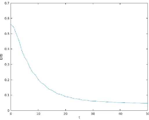
The goal of this section is to develop a stable and convergent numerical method which faithfully describes the behavior of the system. We know, in fact, that the energy of the system decreases in time:

d

dtEˆ(t;y) :=−βyt(0)

Therefore, it is important that the corresponding numerical method preserves the structural property of dissipativity: for longtime computations, the numer-ical scheme must be convergent in classnumer-ical sense, but also yield the correct large time limit. Moreover, the dissipativity of the scheme implies immediately unconditional stability.

3.2.1. Semi-discrete scheme: space discretization

Let Vh ⊂HE1(0,1) be an arbitrary chosen finite dimensional space. We obtain

the following approximating problem:

Problem Gh _{: Findyh∈C}2_{([0,+∞), Vh), i.e.}

ˆ

yh = yh(0),(yh)x(0), yh

∈C2_{([0,+∞), V) verifying:} Z 1

0

(yh)tt(t)(x)wh(x) + ((yh)(t))x(x)(wh)x(x)

dx

+m(yh)tt(t)(0)wh(0) +β(yh)t(t)(0)wh(0) = 0, (51)

with the following initial conditions:

yh(.,0) =yh0∈Vh,

(yh)t(.,0) =yh1∈Vh.

(52)

Discretize [0,1] in p subintervals of same length. Vh ⊂ H1(0,1) then its

elements are globally C[0,1]. Let us consider:

Vh:=

φ∈C[0; 1] : φ_|[xk;xk+1]∈P₂₍R_{), k= 0, . . . , p−1}

,

withxk=kh, k= 0,1, . . . , p. Then dimVh= 2p and note Vh =hφ1, φ2, . . . , φ2pi,

where φi, i = 1, . . . ,2p, are the associated basis functions at nodes xj, j =

0,1₂,1,3₂,2, . . . , p−1₂, respectively.

In this basis, yh(x, t) = yh(t)(x) = P2pj=1Yj(t)φj(x). Replacing yh by his

expression in (51), one obtains:

2p X j=1

Z 1 0

φiφjdx+mφi(0)φj(0)

(Yj)tt(t) + Z 1

0

(φi)x(φj)xdx Yj(t)

+βφi(0)φj(0)(Yj)t(t)

= 0,

for all i= 1,2, . . . ,2p. Finally, we obtain an ordinary differential equation:

A_{Ytt(t) +β}B_{Yt(t) +}K_{Y(t) = 0. (54)}

where

A_{= aij}

1≤i,j≤2p,B= bij

1≤i,j≤2p,K= kij

1≤i,j≤2p, Y = Yi

1≤i≤2p

and

aij =

Z 1 0

φiφjdx+mφi(0)φj(0), bij =φi(0)φj(0), kij =

Z 1 0

(φi)x(φj)xdx.

(55)

Derivation of element matrices. The element matrices are:

A_{e =} h

2



 4 15

2 15 −

1 15 2

15 1615 152 −₁₅1 ₁₅2 ₁₅4



, K_e= 2 h



 7

6 −

4 3

1 6 −4₃ 8₃ −4₃

1

6 −43 76 

,

B_{e =}O_3.

Remark 11. In the definitive expression of matrices, one shall take into account the following parameters:

b11= 1, a11=

2h

15 +m.

Dissipativity of the method. In this paragraph, we demonstrate the dis-sipativity of the semi discrete scheme. Consider the following function:

ˆ

E(t;y) := 1 2

Z 1 0

yt(x, t)2dx+

Z 1 0

yx(x, t)2dx+myt(0, t)2

, (56)

wherey∈ C2_([0,∞);V).

Theorem 12. The solutionyh of the problemGh satisfies: ∀t >0, d

dtEˆ(t;yh) =−β(yh) 2

t(0)≤0. (57)

Proof. For all yh ∈C2([0,∞);Vh), we have:

ˆ

E(t;yh) = 1 2

Z 1 0

(yh)2t(x, t) + (yh)x(x, t)2

dx+m(yh)t(0, t)2

Then we have:

d

dtEˆ(t;yh) = Z 1

0

(yh)x(yh)txdx+ Z 1

0

(yh)t(yh)ttdx+m(yh)t(0)(yh)tt(0). (59)

In other part, by replacingwh by (yh)t in (51), one obtains: Z 1

0

(yh)tt(yh)tdx+ Z 1

0

(yh)tx(yh)xdx=−m(yh)tt(0)(yh)t(0)−β(yh)2t(0). (60)

Then we obtain _dtdEˆ(t;yh) =−β(yh)2_t(0).

3.2.2. Fully discrete scheme

Consider a new variable zh := (yh)t. Rewriting (54) as a first order ODE, we

get:

NU_t=MU

U_{0 = [}Y₀Z_0]⊤_, (61)

where Z _:= Y_{t = [Z1 Z2 . . . Z2p]}⊤ _{be its representation in the basis {φi}i,} U_{= [}Y Z_]⊤_,

N =

I_2p O_2p O_2p A

and M=

O_2p I_2p −K _−βB

.

The time interval is discretized into s equidistant subintervals, for a fixed

s∈N_{. Let ∆t:=T /sdenote the time step and}

tk=k∆t, ∀k∈ {0,1, . . . , s}, (62)

the nodes of the discretization. We adopt as notation Uk

h = [yhkzhk]⊤, the approximation of the solution Uh

at time tk. Let Yk and Zk be the vector representations of yhk and zhk in the

considered basis inVh.

Applying the Crank-Nicholson scheme to the system (61), we obtain:

M U_k+1=S U_{k, (63)}

U_{0= [}Y₀ Z_0]⊤_{, (64)}

for all k= 0,1, . . . , s−1, with

M₌ N

∆t − M

2 =

I2p

∆t −

I2p

2

K

2

A

∆t+β

B

and

S₌ N

∆t+ M

2 =

I2p

∆t

I_2p

2 −K_{2 ∆t}A −βB₂

.

Moreover, for allk= 0,1, . . . , s−1,

Y_k+1−Y_k

∆t =

Z_k+1+Z_k

2 , (65)

AZk+1−Zk

∆t =−K

Y_k+1+Y_k

2 −βB

Z_k+1+Z_k

2 . (66)

Dissipativity of the method. In the following, we show that the scheme (65)-(66) dissipates the norm. The natural norm of Uh =Uh(t) = [yh zh]⊤, the

solution of the semi-discretized system, is defined as:

kUhk2= 1 2

Z 1 0

(yh)2xdx+ Z 1

0

z2_hdx+mzh(0)2

. (67)

We have the following theorem:

Theorem 13. For all k∈N_{, we have:} U k+1 h 2 − U k h 2

=−β∆t

zk+1_h (0) +zk h(0)

2

2

≤0. (68)

Proof. We have:

U k+1 h 2 − U k h 2 = 1 2 Z 1 0

((yh)k+1_x )2−((yh)k_x)2

dx+

Z 1 0

(z_hk+1)2

−(z_hk)2

dx+m

(z_hk+1)2(0)−(z_hk)2(0)

.

Using Crank-Nicholson scheme, one obtains:

y_hk+1−yk h

∆t =

z_hk+1+zk h

2 . (69)

Multiplying (69) by z_hk+1−zk

h and integrating it over [0; 1], we have:

1 2

Z 1 0

(z_hk+1)2−(z_hk)2

dx=

Z 1 0

yk+1_h −yk h

∆t z

k+1 h −z

k h

Moreover, using Crank-Nicholson scheme on (11), we obtain:

Z 1 0

z_hk+1−zk h

∆t wh+

(y_hk+1)x+ (ykh)x

2 (wh)x

dx

+βz k+1

h (0) +zkh(0)

2 wh(0) +m

z_hk+1(0)−zk h(0)

∆t wh(0) = 0. (71)

Substituting wh by yk+1_h and next byyhk in (71), one has:

1 2

Z 1 0

((yh)k+1_x )2dx=−1

2

Z 1 0

(yh)k+1_x (yh)k_xdx− Z 1

0

z_hk+1−zk h

∆t y

k+1 h dx −mz

k+1

h (0)−zhk(0)

∆t y

k+1

h (0)−β

z_hk+1(0) +zk h(0)

2 y

k+1

h (0), (72)

1 2

Z 1 0

((yh)k_x)2dx=−1

2

Z 1 0

(yh)k+1_x (yh)k_xdx− Z 1

0

zk+1_h −zk h

∆t y

k hdx −mz

k+1

h (0)−zkh(0)

∆t y

k

h(0)−β

z_hk+1(0) +zk h(0)

2 y

k

h(0). (73)

Substracting (73) from (72) yields:

1 2

Z 1 0

(yh)k+1x )2−(yh)kx)2

dx

=−1

2

Z 1 0

(z_hk+1)2−(z_hk)2

dx−m

2

zk+1_h (0)2−z_hk(0)2

−β∆t

4

z_hk+1(0) +zk_h(0)

2 . (74) Finally: U k+1 h 2 − U k h 2

=−β∆t

z_hk+1(0) +zk h(0)

2

Figure 1: Energy dissipation E(t)

4. Errors estimates

4.1. A-priori error estimates for the semi-discrete scheme

In this paragraph, we derive the a-priori estimates for the Galerkin solution of (51)-(52), where the discrete spaceVh is the space ofP2 Lagrange polynomials.

These estimates are based on the method used in Choo et al. [18]. The Lagrange interpolation of the weak solution y∈Vh is denoted by ˜y:

˜

y(x, t) =

p−1 X j=0

y(xj, t)φ2j+1(x) +y(x_j+1

2, t)φ2j+2(x)

.

Suppose that

Then for almost every t, we have (cf. Brenner et al. [3], Choo et al. [18]):

ky−yk˜ _H1_(0,1) ≤Chkyk_H2_(0,1),

kyt−y˜tkH1_(0,1) ≤Chkytk_H2_(0,1),

kytt−y˜ttkL2_(0,1) ≤Chkyttk_H1_(0,1).

(76)

The error of the semi-discrete solution yh is defined as

ǫh_:=y

h−y˜∈Vh. Using (51), it follows: Z 1

0

ǫh_ttwdx+

Z 1 0

ǫh_xwxdx+mǫh_tt(0)w(0) +βǫh_t(0)w(0)

=

Z 1 0

(ytt−ytt˜ )wdx+

Z 1 0

(yx−yx˜ )wxdx,

for all w∈Vh, t >0. Using w=ǫh

t, we obtain: Z 1

0 ǫh

ttǫhtdx+ Z 1

0 ǫh

xǫhtxdx= Z 1

0

(ytt−y˜tt)ǫhtdx+ Z 1

0

(yx−y˜x)ǫhtxdx −βǫh_t(0)2−mǫh_tt(0)ǫh_t(0)

≤ Z 1

0

(ytt−ytt˜ )ǫhtdx+ Z 1

0

(yx−yx˜ )ǫhtxdx −mǫh

tt(0)ǫht(0) (77)

for almost everyt∈[0, T]. Then, for almost every t∈[0, T] we have:

d dtEˆ(t;ǫ

h_{) =} Z 1

0

(ytt−ytt˜ )ǫh_tdx+

Z 1 0

(yx−yx˜ )ǫh_txdx−βǫh_t(0)2

≤ Z 1

0

(ytt−ytt˜ )ǫh_tdx+

Z 1 0

(yx−yx˜ )ǫh_txdx. (78) Integrating the previous expression over [0, t]. It follows:

ˆ

E(t;ǫh)≤Eˆ(0;ǫh(0)) +

Z t 0

Z 1 0

(ytt−ytt˜ )ǫh_tdx+

Z 1 0

(yx−yx˜ )ǫh_txdx

ds.

After performing partial integration, one has:

ˆ

E(t;ǫh_{)≤ Eˆ(0;ǫ}h_{(0)) +} Z t

0 Z 1

0

(ytt−y˜tt)ǫhtdx− Z 1

0 ǫh

x ytx−y˜tx

dx

ds

+

Z 1 0

(yx(x, t)−y˜x(x, t))ǫhx(x, t)dx− Z 1

0

Applying the Cauchy-Schwarz and Young inequalities to the second member of the previous inequality, we obtain for allη >0:

ˆ

E(t;ǫh_)≤Eˆ(0;ǫh_{(0)) +η}

kytt−y˜ttk2L2_(0,T;L2_(0,1))+ky_t−y˜tk2_L2_(0,T;H1_(0,1))

+kyx(., t)−yx˜ (., t)k2_L2_(0,1)+kyx(.,0)−yx˜ (.,0)k2_L2_(0,1)

+ 1 4η

Z t 0

ˆ

E(s;ǫh(s))ds+ ˆE(t;ǫh(t)) + ˆE(0;ǫh(0))

.

This leads to:

1− 1

4η

ˆ

E(t;ǫh(t))≤

1 + 1 4η

ˆ

E(0;ǫh(0))

+ 1

4η Z t

0

ˆ

E(s;ǫh(s))ds+η

kytt−yttk˜ 2_L2_(0,T;L2_(0,1))

+kyt−ytk˜ 2_L2_(0,T;H1_(0,1))+ 2ky−yk˜ 2_C([0,T];H1_(0,1))

.

Take η= 1. Using (76), we obtain:

ˆ

E(t;ǫh(t))≤ 5

3Eˆ(0;ǫ

h_{(0)) +}1

3

Z t 0

ˆ

E(s;ǫh(s))ds

+Ch2

kyttk2_L2_(0,T;H1_(0,1))+kytk2_L2_(0,T;H2_(0,1))+kyk2_C([0,T];H2_(0,1))

. (79)

Applying the Gronwall inequality to (79), one obtains:

ˆ

E(t;ǫh(t))≤ C

ˆ

E(0;ǫh(0)) +h2

kyttk2_L2_(0,T;H1_(0,1))+kytk2_L2_(0,T;H2_(0,1))

+kyk2_C([0,T];H2_(0,1))

.

Finally, we have the following result:

Theorem 14. Suppose (75), and take Vh the space of the piecewise P2

Lagrange polynomials. For yh ∈C2([0, T];Vh)solving (51)-(52), we have:

ˆ

E(t;yh−y)12 ≤ C

ˆ

E(0;ǫh(0))12 +h

+kytk_L2_(0,T;H2_(0,1))+kyk_C([0,T];H2_(0,1))

. (80)

In addition, ify0

handyh1 are Lagrange interpolations ofy0andy1, then we have:

ˆ

E(t;yh−y)12 ≤ Ch

kyttk_L2_(0,T;H1_(0,1))+kytk_L2_(0,T;H2_(0,1))

+kyk_C([0,T];H2_(0,1))

. (81)

4.2. A-priori error estimates for the fully discrete scheme

In this paragraph, a-priori error estimates are given for the scheme (65)-(66). Assume thaty ∈H4(0, T;H_E1(0,1)). Let ˘y∈Vh be the projection of the weak solution y, such that:

a(y(t)−y˘(t), wh) = 0, ∀wh∈Vh,

for allt∈[0;T]. One verifies that ˘y∈H4(0, T;H_E1(0,1)) because the projection

y 7→ y˘is bounded in H_E1(0,1). Moreover, let ye _{:= y−y˘ be the error of the}

projection. Suppose that y ∈ H2_{(0, T;H}2

E(0,1)). We have (cf. Strang et al.

[6]):

kye_k

H1_(0,1)≤Chkyk_H2_(0,1),

kye

tkH1_(0,1) ≤Chkytk_H2_(0,1),

kye

ttkH1_(0,1)≤Chkyttk_H2_(0,1).

(82)

Let U(tk) = y(tk);yt(tk) ⊤

denote the weak solution of (14) at time tk

and Uk _{= y}k_;zk

the k-th iteration of the fully discrete scheme (65)-(66) approximatingU(tk). Then the approximating error is defined by:

Ψk :=yk−y˘(tk), Φk:=zk−y˘t(tk),

and Uk

e := Ψk; Φk

, for all k∈ {0,1, . . . , s}.

Theorem 15. Suppose that

y∈H2(0, T;HE2(0,1))∩H4(0, T;HE1(0,1)).

Letk∈ {1, . . . , s}. Then we have:

U

k_−U(t k)

≤C

U_e0

+hkyk

H2 _0,T;H2_(0,1)

+ ∆t3₂

kyttk

H2 _0,T;H1_(0,1)+kyttk_L2 _0,T;H2_(0,1)

.

Proof. Letk∈ {0,1, . . . , s}. The Taylor theorem yields:

∀x∈[0,1], y˘(x, tk+1)−y˘(x, tk)

∆t =

˘

yt(x, tk+1) + ˘yt(x, tk)

2 + ∆tT

k

1(x), (84)

with

Tk 1(x) =

Z tk+1

t

k+ 1₂

˘

yttt(x, t)

2(∆t)2 tk+1−t 2

dt+

Z t

k+ 1 2

tk ˘

yttt(x, t)

2(∆t)2 tk−t 2

dt

− Z tk+1

t

k+ 1₂

˘

yttt(x, t)

2∆t tk+1−t

dt+

Z t

k+ 1 2

tk ˘

yttt(x, t)

2∆t tk−t

dt.

From (84), one verifies:

Ψk+1−Ψk

∆t + ∆tT

k 1 =

Φk+1+ Φk

2 . (85)

Multiplying the previous expression by Φk+1−Φk

and integrating it over [0,1] yields:

Z 1 0

Ψk+1_−Ψk

∆t Φ

k+1_−Φk dx= 1

2

Z 1 0

(Φk+1)2−(Φk)2

dx

−∆t Z 1

0

T₁k(x) Φk+1−Φk dx.

In addition, substitutingtby t_k+1

2 in (11) and using the Taylor expansion, we

obtain:

Z 1 0

yt(x, tk+1)−yt(x, tk)

∆t w(x)dx+

Z 1 0

yx(x, tk+1) +yx(x, tk)

2 wx(x)dx

+

myt(0, tk+1)−yt(0, tk)

∆t +β

yt(0, tk+1) +yt(0, tk)

2

w(0) = ∆tT₂k(w), (86) where the functionalTk

2 :HE1(0,1) →Ris defined by: T₂k(w) =

Z 1 0

Z tk+1

t

k+ 1₂

ytttt(x, t)

2(∆t)2 tk+1−t 2

dt

+

Z t

k+ 1₂

tk

ytttt(x, t) 2(∆t)2 tk−t

2 dt

w(x)dx

+

Z 1 0

Z tk+1

t

k+ 1₂

yttx(x, t)

2∆t tk+1−t

dt− Z t

k+ 1₂

tk

yttx(x, t) 2∆t tk−t

dt

+m

Z tk+1

t_{k+ 1}

2

ytttt(0, t)

2(∆t)2 tk+1−t 2

dt+

Z t_{k+ 1}

2

tk

ytttt(0, t)

2(∆t)2 tk−t 2

dt

w(0)

+β

Z tk+1

t_{k+ 1}

2

yttt(0, t)

2∆t tk+1−t

dt− Z t

k+ 1 2

tk

yttt(0, t)

2∆t tk−t

dt

w(0). (87)

Now, from (66) and (86), one has for all wh∈Vh:

Z 1 0

Φk+1−Φk

∆t whdx+ Z 1

0

Ψk+1_x + Ψk x

2 (wh)xdx+

mΦ

k+1_(0)−Φk₍₀₎

∆t

+βΦ

k+1_{(0) + Φ}k₍₀₎

2

wh(0) =Gk(wh)−∆t T₂k(wh), (88)

where the functionalGk_(w

h) is defined as: Gk(wh) :=

Z 1 0

ye

t(x, tk+1)−yet(x, tk)

∆t whdx

+

my

e

t(0, tk+1)−yet(0, tk)

∆t +β

ye

t(0, tk+1) +yet(0, tk)

2

wh(0).

(89)

Taking wh = ∆t₂ Φk+1+ Φk

∈Vh in (88), yields:

1 2

Z 1 0

(Φk+1)2−(Φk)2dx

=−∆t

2

Z 1 0

Ψk+1_x + Ψk x

2

Φk+1_x + Φk_x dx

−∆t

2

Φk+1(0) + Φk(0)

mΦ

k+1_(0)−Φk₍₀₎

∆t +β

Φk+1(0) + Φk₍₀₎

2

+∆t 2 G

k_(Φk+1_{+ Φ}k₎₋(∆t)2

2 T

k

2(Φk+1+ Φk). (90)

Then we have:

U k+1 e 2 − U k e 2 = 1 2 Z 1 0

(Ψk+1x )2−(Ψkx)2

dx

−∆t

2

Z 1 0

Ψk+1_x + Ψk

2

Φk+1_x + Φk_x

dx−β∆t

4

Φk+1(0) + Φk(0)

2

+∆t 2 G

k_(Φk+1_{+ Φ}k₎₋(∆t)2

2 T

k

2(Φk+1+ Φk) ≤ 1

2

Z 1 0

(Ψk+1x )2−(Ψkx)2

dx−∆t

2

Z 1 0

Ψk+1 x + Ψk

2

Φk+1x + Φkx

+∆t 2 G

k_(Φk+1_{+ Φ}k₎₋(∆t)2

2 T

k

2(Φk+1+ Φk). (91)

Now by (85), we obtain:

Z 1 0

Ψk+1 x + Ψk

2

Φk+1x + Φkx dx = Z 1 0 (Ψk+1

x )2−(Ψkx)2

∆t dx+ ∆t

Z 1 0

(T₁k)x

Ψk+1_x + Ψk_x

dx.

Then we get:

U k+1 e 2 − U k e 2

≤ −(∆t) 2

2

Z 1 0

(T₁k)x

Ψk+1_x + Ψk_x

dx

+∆t 2 G

k_(Φk+1_{+ Φ}k₎₋ (∆t)2

2 T

k

2(Φk+1+ Φk); (92)

It can easily be seen that:

T k 1 2

H1_(0,1)≤∆t

Z tk+1

tk

kyttt˘ (t)k2_H1_(0,1)dt≤C∆t

Z tk+1

tk

kyttt(t)k2_H1_(0,1)dt.

(93)

Rewriting the second term of Tk

2(w) (using the fact w(1) = 0), one obtains: Z 1

0

Z tk+1

t_{k+ 1}

2

yttx(x, t)

2∆t tk+1−t

dt− Z t

k+ 1₂

tk

yttx(x, t) 2∆t tk−t

dt

wx(x)dx

=

Z t

k+ 1₂

tk

tk−t

2∆t

yttx(0, t)w(0) + Z 1

0

yttxx(x, t)w(x)dx

dt

− Z tk+1

t

k+ 1₂

tk+1−t

2∆t

yttx(0, t)w(0) +

Z 1 0

yttxx(x, t)w(x)dx

dt.

Then we have:

T₂k(Φk)≤C Φ k 2

L2_(0,1)+|Φ

k_(0)|2_{+ ∆t}Z tk+1 tk

kytttt(t)k2_H1_(0,1)

+kyttt(t)k2H1_(0,1)+ky_tt(t)k2_H2_(0,1)

dt

. (94)

Additionally, using the Cauchy-Schwarz and Young inequalities, yields:

|Gk_(Φk+1_{+ Φ}k_{)| ≤ C}

Φ

k+1_{+ Φ}k 2

L2_(0,1)+|Φ

+ 1 ∆t

Z tk+1

tk

kyett(t)k2L2_(0,1)+|y_tte(0, t)|2

dt+kyetk2C([tk;tk+1];H1(0,1))

. (95)

Using the expressions (92)-(95), one obtains:

U k+1 e 2 − U k e 2 ≤C ∆t U k+1 e 2 + U k e 2

+∆tkyetk2C([tk;tk+1];H1(0,1))+

Z t_k+1

tk

kyett(t)k2L2_(0,1)+|y_tte(0, t)|2

dt

+(∆t)3

Z tk+1

tk

kytttt(t)k2_H1_(0,1)+kyttt(t)k2_H1_(0,1)+kytt(t)k2_H2_(0,1)

dt

. (96)

Let m ∈ {0,1, . . . , s}. Suppose that ∆t ≤ _2C1 (with C from (96)). Summing (96) over k∈ {0,1, . . . , m}, gives:

1 2

U_em+1

2 ≤ 3 2 U_e0

2 +C ∆t m X k=1 U k e 2

+kye

tk2C([0,T],H1_(0,1))

+kye

ttk2L2_(0,T;H1_(0,1))+ ∆t

3

kyttttk2_L2_(0,T;H1_(0,1))

+kytttk2_L2_(0,T;H1_(0,1))+kyttk2_L2_(0,T;H2_(0,1))

.

(97)

Finally, due to the discrete in time Gronwall inequality and (84), we obtain:

U_em+1

2 ≤C U_e0

2

+h2 kytk2_C([0,T],H2_(0,1))+kyttk2_L2_(0,T;H2_(0,1))

+ ∆t3 kyttttk2_L2_(0,T;H1_(0,1))+kytttk2_L2_(0,T;H1_(0,1))

+kyttk2_L2_(0,T;H2_(0,1))

.

(98)

The result now follows from the previous expression, (82) and the triangle inequality.

References

[1] A. Pazy, Semigroups of Linear Operators and Applications to Partial Dif-ferential Equations, Springer-Verlag, New York (1983).

[3] S.C. Brenner, L.R. Scott, The Mathematical Theory of Finite Element Methods, Springer Science + Business Media, New York (2008).

[4] H. Brezis, Analyse Fonctionnelle, Th´eorie et Applications, Masson, Paris (1983).

[5] P.G. Ciarlet, Introduction l’Analyse Num´erique Matricielle et l’Optimisation, Masson, Paris (1982).

[6] G. Strang, G. Fix, An Analysis of the Finite Element Method, Prentice-Hall, Englewood Cliffs, New Jersey (1973).

[7] G.H. Golub, C.F. Van Loan, Matrix Computations, The Johns Hopkins University Press, Baltimore (1989).

[8] J.L. Lions, E. Magenes, Nonhomogeneous Boundary Value Problems and Applications, Vol. 1, Springer, New York (1972).

[9] Z.H. Luo, B.Z. Guo, ¨O. M¨orgul, Stability and Stabilization of Infinite Di-mensional Systems with Applications, Springer, London (1999).

[10] M.A. Naimark, Linear Differential Operators, Vol. 1, Springer, New York (1967).

[11] R. Temam, Infinite Dimensional Dynamical Systems in Mechanics and Physics, Vol. 68, Springer-Verlag, New York (1988).

[12] J. Rappaz, M. Picasso, Introduction l’Analyse Num´erique, Presses Poly-techniques et Universitaires Romandes, New York (1998).

[13] F.Z. Saouri, Stabilisation de Quelques Syst`emes ´Elastiques. Analyse Spec-trale et Comportement Asymptotique, Th`ese de l’Universit´e Henry Poincar´e - Nancy I (2000).

[14] M. Miletic, Stability Analysis and a Dissipative FEM for an Euler-Bernoulli Beam with Tip Body and Passivity-Based Boundary Control, PhD Thesis, Vienna University of Technology (2015).

[15] A. Shkalikov, Boundary problem for ordinary differential operators with parameter in boundary conditions,J. Sov. Math.,33(1986), 1311-1342. [16] B. Chentouf, J.M. Wang, Optimal energy decay for a nonhomogeneous

[17] K.A. Tour´e, E.P. Mensah, M.M. Taha, Stabilization and Riesz basis prop-erty for an overhead crane model with feedback in velocity and rotating velocity,Journal of Nonlinear Analysis Application, 2014 (2014), 1-14. [18] S.M. Choo, S.K. Chung, R. Kannan, Finite element Galerkin solutions