A Study on Path Loss and Shadowing for Wireless
Communication Channels
Zachary Bosire Omariba1, 2,*
1National Centre for Material Service Safety, University of Science and Technology Beijing-100083 PRC 2Computer Science Department, Egerton University, Egerton-20115 Kenya
*Corresponding Author: [email protected], +254-729154296 Dr. Nelson Bogomba Masese3
3Kabarak University. Nakuru- 20100 Kenya [email protected], +254-727171725
Abstract-The demand for accelerated speed, anywhere, and any time connectivity has made wireless communication networks increasingly dense. This has resulted into intense research on how speed of data transfer, security of data, spectrum sharing, and storage of the big data realized can be improved in an efficient way. However the major challenge which has necessitated continuous research progress in the subject is the study of communication path loss and shadowing and how it can be eliminated or lessened to improve the channels involved. This paper will perform experiments on radio propagation models, ray tracing models and perform its simulations in Matlab, as well as provide a review of the various path loss models. The simulation results obtained indicated that when the receiver far away from the transmitter, the signal begins to be weaker and weaker until it is lost. However if the receiver will move away from a closer base station, and while the signal is weakening, it encounters another base station, the two base stations performs a handshake and the signal will start gaining strength.
Keywords: communication channels, Path loss and shadowing, radio-wave propagation, ray tracing
I. INTRODUCTION
Wireless communication is progressing at an accelerated speed as anytime, anywhere connectivity is becoming a reality, and wireless networks are becoming increasingly dense [1]. This is attributed to the push for demand for higher and higher wireless data rates from modern wireless devices such as smartphones, tablets [2] and other consumer electronics which causes a significant stress to existing wireless networks for accelerated need for radio spectrum [3]. Despite this improvements in radio spectrum and spectrum sharing, there still remains a challenge of path-loss and shadowing which is caused by various barriers [4]. In wireless communication path loss refers to the mean level of the received signal, whereby a wave travelling some distance is described. The relation between the signal power and distance
of propagation in wireless communication channels is modelled by the wireless path loss techniques. Following the inverse square law, the signal power drops exponentially as it moves away from its source, and the wave scatters and disperses as it moves towards the receiver, resulting to only a fraction of signal is received at the receiver end [5].
Path loss is caused by dissipation of power radiated by the transmitter as well as effects of the propagation channel. Thus the path loss can be basically due to free space loss, ground reflection, reflection and diffraction, microcellular propagation and indoor propagation. The value of the path loss cannot be analytically determined in multipath environments, but by numerical path loss models which estimate the mean signal level received for various scenarios. When these waves travel through a channel they encounter fading phenomena called shadowing [6][7], which occurs due to partial or complete blockage by obstacles which are larger than the signal wavelength. However wireless channels used for the radio wave propagation over the sea surface are different from the usual
channels used in ground-to-ground
deterioration [10]. Antenna gains and cable losses are taken into consideration for path loss estimation. The three major losses between the base station and the receiver comprises of path loss, shadowing and fast fading. Knowing the transmitted and received power the measured path loss is given as:
t t thh (1)
where PT andGb are the transmitted power and gain of the base station,Lc is the cable loss,Gm is the gain of the mobile station and RSS is the Received Signal Strengths. Since path loss and shadowing occur over relatively large distances, they are referred to as large-scale propagation effects. The path loss calculated from the measurements is used as a reference for assessing the performance of the propagation models. This paper is organised as follows: Section 2 will provide radio propagation models; Section 3 will provide the transmitter-receiver signal models; Section 4 and Section will provide free space path loss and Ray tracing respectively. We used MATLAB to simulate the free-space and Ray tracing models respectively. Finally Section 6 is the conclusion of the study.
II. BACKGROUND INFORMATION A propagation model is a set of mathematical expressions, diagrams, and algorithms used to represent the radio characteristics of a given environment[11]. The initial understanding of radio wave propagation goes back to the pioneering work of James Clerk Maxwell, who
in 1864 formulated the theory of
electromagnetic propagation which predicted the existence of radio waves. In1887, the physical existence of these waves was demonstrated by Heinrich Hertz. In 1894 Oliver Lodge used these principles to build the first wireless communication system, however its transmission distance was limited to 150 meters. By 1897 the entrepreneur Guglielmo Marconi had managed to send a radio signal from the Isle of Wight to a tugboat 18 miles away, and in 1901 Marconi’s wireless system could traverse the Atlantic Ocean. These early systems used
telegraph signals for communicating
information. The first transmission of voice and music was done by Reginald Fessenden in 1906
using a form of amplitude modulation, which got around the propagation limitations at low frequencies observed by Hertz by translating signals to a higher frequency, as is done in all wireless systems today.
From the early developments in wireless systems, electromagnetic waves propagate through environments where they are reflected, scattered, and diffracted by walls, terrain, buildings, and other objects [11][12]. The ultimate details of this propagation can be obtained by solving Maxwell’s equations with boundary conditions that express the physical characteristics of these obstructing objects. The indoor radio propagation is not hampered by weather controlling parameters such as heavy rain, floods, clouds, or snowfall as outdoor; nevertheless the indoor building-walls, items of furniture, windows, doors, and other household items can affect it [13]. Since these calculations are difficult, and many times the necessary parameters are not available, approximations have been developed to characterize signal propagation without resorting to Maxwell’s equations. The most common approximations use ray-tracing techniques. These techniques approximate the propagation of electromagnetic waves by representing the wave fronts as simple particles: the model determines the reflection and refraction effects on the wave-front but ignores the more complex scattering phenomenon predicted by Maxwell’s coupled differential equations. The simplest ray-tracing model is the two-ray model, which accurately describes signal propagation when there is one direct path between the transmitter and receiver and one reflected path.
III. TRANSMITTER-RECEIVER SIGNAL MODELS
Our models are developed mainly for signals in the UHF and SHF bands, from 0.3-3 GHz and 3-30 GHz. All transmitted and received signals we consider are real. The transmitted signal is modelled as:
cos t sin
t cos sin
Where ( ) t( ) ( is a complex baseband signal with in-phase component
x(t)= ( , quadrature component y(t) = ( ,bandwidth , power . We callu(t)
the complex envelope of s(t). The power in the transmitted signals(t)is pt pu/ .
The received signal will have a similar form:
( ) ( ) (3)
Where the complex baseband signal v(t) will depend on the channel through which s(t) propagates.
The received signal may have a Doppler shift of
h /λ associated with it, where θ is the arrival angle of the received signal relative to the direction of motion, v is the receiver velocity towards the transmitter in the direction of motion, and λ is the signal wavelength.
IV. FREE SPACE PATH LOSS
Free-space is a boundary-less medium with a
speed of signal propagation
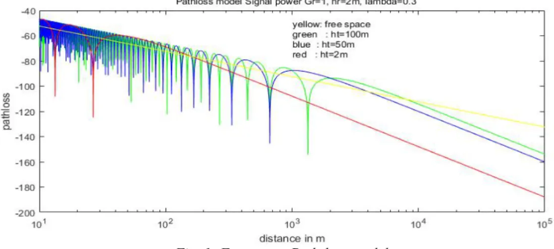
[14][15]independent of position and directions as the signal propagates in a straight line from source to destination. Free space impairments of propagating signal can cause a decline in power density of a given electromagnetic wave due to like height, structures, propagation channels, attenuation, refractions, position, location, and absorption[16][10][17]. The two-ray model takes into account a line-of-sight and a ground reflection. It is a good approximation for propagation over a smooth well-reflecting terrain, as modelled by the plane-earth model. MATLAB is used to simulate the Free-space Path-loss model as shown in Fig.. 1
Fig. 1: Free space Path-loss model
From Fig. 1 the free-space path-loss is represented by the yellow line and the rest shows the path between the receiver and transmitter over different distances. The path is lost as the distance increases as demonstrated in the Fig..
V. RAY TRACING
The most common approximations use ray-tracing techniques. These techniques approximate the propagation of electromagnetic waves by representing the wave fronts as simple particles. The model determines the reflection and refraction effects on the wave-front but ignores the more complex scattering phenomenon predicted by Maxwell’s coupled
differential equations [18]. Two-Ray model is the simplest ray tracing model which accurately describes signal propagation when there is one direct path between the transmitter and receiver and one reflected path. Ray tracing techniques will therefore approximate the propagation of electromagnetic waves by representing the wave-fronts as simple particles. This means that the diffraction, reflection, and scattering effects on the wave-front are approximated using simple geometric equations instead of Maxwell’s more complex wave equations. A. Two-Ray Tracing Model
Fig. 2: The two-ray model
In the two-ray model the reflected path will bounce back off the ground and the two-ray model becomes handy in propagation approximations along rural roads, highways, and over water.
(4)
t Δ
t t (5)
o o
o( ) (6)
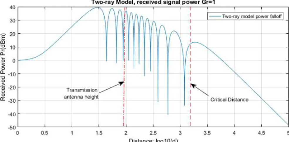
A plot of Equation 3 as a function of distance is illustrated in Fig. 2 with parameter given as: f = 1800MHz, R=-1, ht = 100m, hr = 1m, Gl = 1, Gr = 1 and transmit power normalized so that the plot starts at 0 dBm.
From Fig.3 it is shown that the power near the transmitting station increases rapidly and starts to fluctuate with the increase of the distance from the transmitting station. Thus the transmission power is steady when the receiver is close to the transmitter. The power falloff with distance in the two-ray model can be approximated by averaging out its local maxima and minima. This results in a piecewise linear model with three segments, which is also shown in Fig. 3 slightly offset from the actual power falloff curve for illustration purposes. In the first segment power falloff is constant and proportional to /( ) , for distances between ht and dc power falls off at -20 dB/decade, and at distances greater than dc power falls off at -40 dB/decade.
Fig. 3: Two-Ray Model: Receiver Signal Power Model
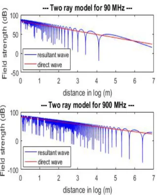
The simulations performed for Two-ray tracing model under variant dimensions are shown in Fig.4 to Fig.6. It is evident from Fig. 4. Field
faster when the frequency is small, and as the signal frequency improves it becomes strong. The model of two-ray considering path loss vs. distance between antenna shows that the higher the distance the further the free space scatters from the two-ray model as shown in Fig. 5. Consequently in Fig. 6, the path loss rises
steadily with the increase of distance of propagation of signal between antennas. Therefore to improve in the radio-wave propagation, the number of base stations should be closer to each other.
Fig. 4: Two-Ray Ground Reflection Model
Fig. 5: Model of Two Ray Ground Reflection
Fig. 6: Path Loss Propagation
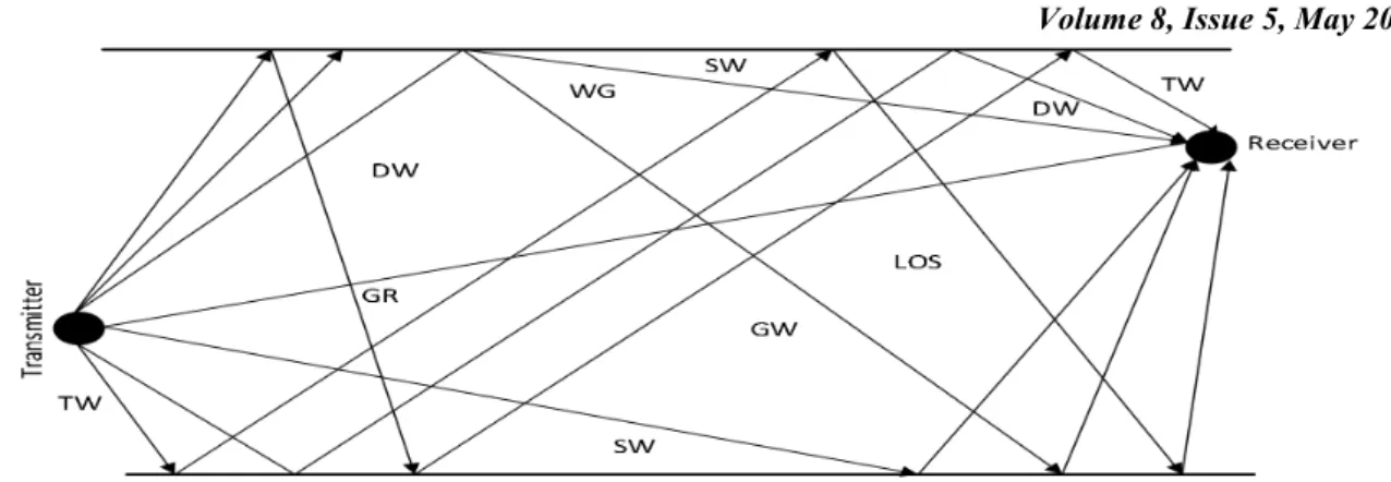
B. Dielectric Canyon (Ten-Ray Model) The Ten-ray model includes all the paths due to single, double and triple reflections[18]: specifically, there is the LOS, the ground-reflected (GR), the single-wall (SW) reflected, the double-wall (DW) reflected, the triple-double-wall (TW)
12
Fig. 7: Overhead View of the Dielectric Canyon (Ten-Ray) Model
For the Dielectric Canyon model, the received signal is given by:
m ( )
/
t t ( ) t / (7)
Then the received power corresponding to Equation 5 is shown as:
t t Δ
t (8)
C. General Ray Tracing
The General Ray Tracing (GRT) can be used to predict field strength and delay spread for any building configuration and antenna placement. It explains the basic mechanism of urban propagation, and can be used to obtain delay and signal strength
information for a particular transmitter and receiver configuration in any given environment. The GRT method uses geometrical optics to trace the propagation of the LOS and reflected signal components. The LOS and reflected paths provide the dominant components of the received signal, since diffraction and scattering losses are high. Diffraction occurs when the transmitted signal “bends around” an object in its path to the receiver, as shown in Fig. 8. Wedge diffraction simplifies the geometrical theory of diffraction (GTD) by assuming the diffracting object is a wedge rather than a more general shape. Diffraction is most commonly modeled by the Fresnel knife edge diffraction model due to its simplicity.
Fig. 8: Fresnel Knife-edge diffraction
In particular, this model does not consider diffraction parameters such as polarization, conductivity, and surface roughness, which can lead to inaccuracies. The geometry of Fig. 7 indicates that the diffracted signal travels distance
resulting in a phase shift of
( )/ , for h small relative to d and d’, the signal must travel an additional distance relative to the LOS path of
approximately: Δ and the
13 All Rights Reserved © 2019 IJARCSEE
where
( )… (10)
is called the Fresnel-Kirchoff diffraction parameter. The path loss associated with knife-edge diffraction is generally a function of v. However, computing this diffraction path loss is fairly complex, approximations for knife-edge diffraction path loss (in dB) relative to LOS path loss are given by Lee as:
t
lg . . . Ͳ
lg . . Ͳ
lg . . ( . . ) Ͳ .
lg . / v > .
(11) The knife-edge diffraction model yields the following formula for the received diffracted signal:
t ( )/
(12) where is the antenna gain and
Δ / is the delay associated with the diffracted ray relative to the LOS path. In addition to diffracted rays, there may also be rays that are diffracted multiple times, or rays that are both reflected and diffracted. Models exist for including all possible permutations of reflection and diffraction; however, the attenuation of the corresponding signal components is generally so large that these components are negligible relative to the noise. Diffraction models can also be specialized to a given environment.
D. Local Mean Received Power
Local mean receiver power is the path loss computed from all ray tracing models is associated with a fixed transmitter and receiver location. In addition, ray tracing can be used to compute the local mean received power in the vicinity of a given receiver location by adding the
The processing time required to predict the mean receiver power strength of an indoors environment follows a polynomial distribution as the number of walls or obstacles increases [19].
VI. PATH-LOSS MODELS
There are various path-loss models for radio propagation channels. They include Okumura model, Lee’s model, Hata model, Cos 231 extension to Hata model and Multi-slope or Linear piecewise model. These models are explained below:
A. Okumura model
This model is applicable over distances of 1-100 Km and frequency ranges of 150-1500 MHz. The base station heights for these measurements were 30-100m, and thus the empirical path loss formula of Okumura at distance d parameterized by the carrier frequencyfc[20] is given by:
t t
th (13)
where:
t : is free space path loss at distance d and carrier frequency
is the median attenuation in addition to free space path loss across all environments
: is the mobile antenna height gain factor
: is the base station antenna height gain factor
th :is the gain due to the type of environment
From the Okumura’s empirical plots, the
values of and th are
14 (14)
lg
lg / Ͳ (15)
B. Hata model
The Hata model is an empirical formulation of the graphical path loss data provided by Okumura and is valid over roughly the same range of frequencies, 150-1500MHz. This empirical model simplifies calculation of path loss [20]since it is a closed-form formula and is not based on empirical curves for the different parameters. The standard formula for empirical path loss in urban areas under the Hata model is:
t m䁗 . . lg
. lg m .
. lg lg ( ) (16) where: m is the is a correction factor for the mobile antenna height based on the size of the coverage area. For small to medium sized cities, this factor is given by:
m . o . . o .
(17) and for larger cities at frequencies fc> 300 MHz by:
m . lg ( . ) . (18)
The Okumura model is well approximated by the Hata model for distances d > 1 Km. Thus, it is a good model for first generation cellular systems, but does not model propagation well in current cellular systems with smaller cell sizes and higher frequencies.
C. COST 231 extension to Hata model (CM)
This model is referred to as the COST 231 extension to the Hata model, and is restricted to the following range of parameters: 1.5GHz < fc < 2 GHz, 30m <
ht< 200 m, 1m < hr< 10 m, and1Km < d
< 20 Km. The Hata model was extended
and technical research (EURO-COST) to2 GHz using the following formula [21].
t m䁗 . . o . o
m . . o o (19)
where: a(hr)is the same correction factor as before and CM is 0 dB for medium sized cities and suburbs, and 3 dB for metropolitan areas.
D. Lee’s model
The Lee’s path-loss model is based on empirical data chosen so as to model a flat terrain. Large errors arise when the model is applied to a non-terrain area. However Lee’s model is known to be a “North American model” than that of Hata [20]. To calculate the propagation loss the following formula is used:
t . ho /
ho / (20)
where: d is distance between a transmitter and receiver,fis transmitted frequency and
15 All Rights Reserved © 2019 IJARCSEE
ܭ o /
ܭ o o / >
(21) The path loss exponents, K and dc are typically obtained via a regression fit to empirical data. The multiple equations in the dual-slope model can be captured with the following dual-slope approximation:
ܭ/t( ) (22)
where
t / (23)
The two-slope model can be extended to more than two regions hence the name multi-slope model.
VII. CONCLUSION
The wave for demand of wireless electronic gadgets and devices has become an enabler for the development of wireless
network communications. Various
research are being conducted to improve the efficiency of wireless communications as is witnessed in the recent past. With the confirmation of 5G broadband networks launch by 2020, the demand still is on the rise. However there exists some challenges which research is trying to solve. One of the challenge is path loss and shadowing which is an obstacle to the development of wireless networks. However there is much progress realized than it was two decades ago. This study tried to examine the various ray tracing and path loss models. Some simulations for ray tracing were performed using Matlab and the results presented. The drawback of this study is that simulations were not performed for the path loss models so as to compare their reliability, and that will be covered in the next study.
REFERENCES
[1] B. Sirkeci-mergen and S. Moballegh, ‘Ad Hoc Networks Broadcasting in dense linear networks : To cooperate or not to cooperate ?’, Ad Hoc Networks, vol. 83, pp. 182–197, 2019.
[2] A. Michaloliakos, R. Rogalin, Y. Zhang, K. Psounis,
105, pp. 150–165, 2016.
[3] M. Wellens, J. Riihijärvi, and P. Mähönen, ‘Spatial statistics and models of spectrum use’, Comput. Commun., vol. 32, pp. 1998–2011, 2011.
[4] Z. Ren, G. Wang, Q. Chen, and H. Li, ‘Modelling and simulation of Rayleigh fading , path loss , and shadowing fading for wireless mobile networks’,
Simul. Model. Pract. Theory, vol. 19, pp. 626–637, 2011.
[5] E. D. Kaur and E. H. S. Gill, ‘Pathloss Modelling In MATLAB to Generate’,Int. J. Innov. Res. Sci. Eng. Technol., vol. 5, no. 4, pp. 4697–4707, 2016. [6] A. Raheemah, N. Sabri, M. S. Salim, P. Ehkan, and R.
B. Ahmad, ‘New empirical path loss model for wireless sensor networks in mango greenhouses’,
Comput. Electron. Agric., vol. 127, pp. 553–560, 2016. [7] C. Sommer, S. Joerer, and F. Dressler, ‘On the Applicability of Two-Ray Path Loss Models for Vehicular Network Simulation’,2012 IEEE Veh. Netw. Conf., pp. 64–69, 2012.
[8] A. Habib and S. Moh, ‘Wireless Channel Models for Over-the-Sea Communication : A Comparative Study’,
Appl. Sci., vol. 9, no. 443, 2019.
[9] T. S. Rappaport and S. Deng, ‘73 GHz Wideband Millimeter-Wave Foliage and Ground Reflection Measurements and Models’, in 2015 IEEE International Conference on Communications (ICC), ICC Workshops, 2015, pp. 8–12.
[10] S. Cheerla, D. V. Ratnam, and H. S. Borra, ‘Neural network-based path loss model for cellular mobile networks at 800 and 1800 MHz bands’,Int.J. Electron. Commun. (AEÜ), vol. 94, pp. 179–186, 2018.
[11] S. S. Sidhu, A. Khosla, and A. Sharma,
‘Implementation of 3-D Ray Tracing Propagation Model for Indoor Wireless Communication’, Int. J. Electron. Eng., vol. 4, no. 1, pp. 43–47, 2012. [12] C. Hu et al., ‘Options for Prognostics Methods: A
review of data-driven and physics-based prognostics’, in Annual Conference of the Prognostics and Health Management Society, 2013.
[13] T. K. Geok, F. Hossain, and W. Tan, Alan Chiat, ‘A novel 3D ray launching technique for radio propagation prediction in indoor environments’,PLoS ONE 13(8) e0201905. https//doi.org/ 10.1371/journal.pone.0201905, pp. 1–14, 2018. [14] L. Bing, ‘Study on Modeling of Communication
Channel of UAV’, Procedia Comput. Sci., vol. 107, no. Icict, pp. 550–557, 2017.
[15] L. C. Fernandes, A. José, and M. Soares, ‘Path loss prediction in microcellular environments at 900 MHz’,
Int. J. Electron. Commun., vol. 68, no. 10, pp. 983– 989, 2014.
[16] A. Sari and A. Alzubi,Path Loss Algorithms for Data Resilience in Wireless Body Area Networks for Healthcare Framework, 1st ed. Elsevier Inc., 2018. [17] M. N. Hindia, A. M. Al-samman, T. A. Rahman, and
T. M. Yazdani, ‘Outdoor large-scale path loss characterization in an urban’,Phys. Commun., vol. 27, pp. 150–160, 2018.
[18] A. Bhuvaneshwari, R. Hemalatha, and T.
Satyasavithri, ‘Semi Deterministic Hybrid model for Path Loss prediction improvement’, Procedia -Procedia Comput. Sci., vol. 92, pp. 336–344, 2016. [19] J. Sánchez, C. Castro, and L. Villaseñor, ‘MEAN
RECEIVER POWER PREDICTION FOR INDOORS 802 . 11 WLANS USING THE RAY TRACING TECHNIQUE’, J. Appl. Res. Technol., pp. 33–48, 2011.
[20] M. A. Alim, M. M. Rahman, M. M. Hossain, and A. Al-Nahid, ‘Analysis of Large-Scale Propagation Models for Mobile Communications in Urban Area’,
16
Models- COST 231 final report’, 1999. 2006.
Zachary Bosire Omariba Holds Bsc Computer Science ans Msc Computer Science from Karnatak, and Periyar University in 2004, and 2006 respectively. He is currently a PhD student Computer Science and Technology- University of Science and Technology Beijing. His research interest includes: big data analytics, Prognostics and health management, and systems simulation.