BIVARIATE QUANTILE FUNCTIONS AND THEIR
APPLICATIONS TO RELIABILITY MODELLING
Balakrishnapillai Vineshkumar1
Department of Statistics, Government Arts College, Thiruvananthapuram-695014, India Narayanan Unnikrishnan Nair
Department of Statistics, Cochin University of Science and Technology, Cochin-682022, India
1. INTRODUCTION
Quantile functions are alternatives to distribution functions in specifying probability distributions and can be successfully employed in all forms of statistical analysis. Al-though one can be mathematically derived from the other, quantile functions, which are simple in form and very much flexible, can be generated without reference to the distribution function. This gives a variety of quantile functions to model random phe-nomenon in addition to distribution functions. For the relative advantages of quantile function, its adaptability to modelling and methods of generating quantile functions we refer to Gilchrist (2000) and Nairet al.(2013). There has been a spurt in interest in re-cent times to utilize quantile functions and concepts derived from it in modelling and analysis of lifetime data, and in information theory, see for example Nair and Sankaran (2009), Nair and Vineshkumar (2010, 2011), Franco-Pereiraet al.(2012), Soni and Dewan (2012), Nairet al.(2013), Linet al.(2016), Kumar and Rani (2018), Kayal and Tripathy (2018), Sadeghiet al.(2019) and their references.
Some attempts have been made in the literature to extend the concept of quantile functions to higher dimensions, as can be seen from the works of Chen and Welsh (2002), Serfling (2002), Belzunceet al.(2007) and Cai (2010). However, none of these approaches appear to have been utilized in the context of reliability analysis. Moreover, extenstion of univariate quantiles to represent bivariate life distributions does not seem to have been discussed in the literature. The present work is, therefore, an attempt to discuss a definition of bivariate quantile function appropriate to analyze bivariate lifetime data and to derive some basic results in this connection. This is motivated by extending to the bivariate case the advantages of the univariate quantile-based approach namely, the benefits of alternative methodology, new simple and flexible models, certain new results
that are difficult to find through the distribution function approach, more robust esti-mation procedures and sometimes better insight into the data generating mechanism. In the process, it is conceived that for a nonnegative random vector(X1,X2), the bi-variate quantile function is a pair that transforms the unit square [0, 1]2, to points in
the planex1−x2, where(x1,x2)stands for the realization of(X1,X2). By doing so we ensure that the bivariate results are consistent with quantile-based reliability concepts and results in the univariate case, and also the basic notions in the existing distribution function approach. Based on the proposed bivariate quantile function, we define the bivariate hazard and mean residual quantile functions, and establish some of their prop-erties. Some new flexible quantile functions are suggested and a real data set is modeled with one of them.
The paper is organized into seven sections. In Section 2, some basic definitions and results in univariate case needed for sequel are presented. The definition of bivariate quantile function and some examples form the material in Section 3. This is followed in Section 4 by the discussions on the concepts of bivariate hazard and mean residual quan-tile functions. Section 5 is devoted to the derivation of new models using special forms bivariate hazard and mean residual quantile functions. In Section 6, the application of the results to real data set is considered, and the work is concluded in Section 7.
2. BASIC RESULTS IN THE UNIVARIATE CASE
LetX be a nonnegative random variable with absolutely continuous distribution func-tionF(x), quantile function
Q(u) =inf{x|F(x)≥u}, 0≤u≤1
and the quantile density functionq(u) =d Q(u)
d u . If f(x)is the probability density
func-tion ofX we have the relationship f(Q(u)) = [q(u)]−1. Analogous to the hazard rate
of the random variableX, defined as
h(x) = f(x) 1−F(x),
in the quantile function approach we have the hazard quantile function
H(u) =h(Q(u)) = [(1−u)q(u)]−1,
which determinesQ(u)uniquely as
Q(u) =
Zu
0
d p
(1−p)H(p). Similarly, corresponding to the mean residual function
m(x) = 1 1−F(x)
Z∞
x
the mean residual quantile function is defined as
M(u) =m(Q(u)) = (1−u)−1
Z1
u
(1−p)q(p)d p.
Further
[H(u)]−1=M(u)−(1−u)d M(u) d u and
Q(u) =
Zu
0
M(p)−(1−p)d Md p(p)
1−p d p.
Let X andY be two lifetimes with hazard quantile functions HX(.)andHY(.), and mean residual quantile functionsMX(.)andMY(.), respectively. WhenX andY are to be compared, we say thatX is smaller thanY
1. in hazard quantile function order, written asX ≤H Q Y ifHX(u)≥ HY(u)for
0≤u≤1, and
2. in mean residual quantile function order , denoted by X≤M RQY if MX(u) ≤
MY(u)for 0≤u≤1.
Mathematically 1 and 2 are equivalent respective to the dispersive order and excess wealth order, respectively, although the two have different interpretations and reliability prop-erties. For details see Vineshkumaret al.(2015). It may be noted that the hazard (mean residual) quantile orders mentioned above are different from the usual hazard rate (mean residual life) orders. For detailed study of the concepts and definitions given in this sec-tion we refer to Nairet al.(2013) and Vineshkumaret al.(2015).
3. BIVARIATE QUANTILE FUNCTIONS
Let(X1,X2)be a nonnegative random vector with absolutely continuous distribution functionF(x1,x2), survival function ¯F(x1,x2)and probability density functionf (x1,x2). We denote byFi(xi)( ¯Fi(xi)) the marginal distribution (survival) function ofXi,i=1, 2. The quantile function ofXi is
Qi(ui) =inf{xi|Fi(xi)≥ui}, 0≤ui≤1,i=1, 2. (1)
In defining bivariate quantile functions we seek transformations of points[0, 1]2in the unit square representing theu1−u2plane to points in thex1−x2plane. Our approach, which is slightly different from the existing ones, consists in choosing the quantile func-tions ofP(X1>x1)andP(X2>x2|X1>x1)that makes up the joint distribution func-tion through
¯
The advantage of this approach is that the terms on the right are more convenient to define various reliability functions.
DEFINITION1. The bivariate quantile function of (X1,X2) is defined as the pair
(Q1(u1),Q21(u2|u1)), where Q1(u)is as given in (1) and
Q21(u2|u1) =inf{x2|P(X2≤x2|X1>Q1(u1))≥u2}. (2)
EXAMPLE2. For the Gumbel’s bivariate exponential distribution ¯
F(x1,x2) =exp[−λ1x1−λ2x2−θx1x2],x1,x2>0; λ1,λ2>0, 0≤θ≤λ1λ2
F1(x1) =1−exp[−λ1x1]gives Q1(u1) =−log(1−
u1)
λ1 . Also
P(X2>x2|X1>x1) =e−(λ2+θx1)x2
has quantile function
Q21(u2|u1) = −λ1log(1−u2) λ1λ2−θlog(1−u1)
.
EXAMPLE3. Consider the bivariate Pareto distribution with survival function ¯
F(x1,x2) = (1+a1x1+a2x2+b x1x2)−p, x1,x2>0,a1,a2>0, 0≤b≤(p−1)a1a2.
The marginal distribution function of X1is
F1(x1) =1−(1+a1x1)−p,
which yields
Q1(u1) = 1
a1(1−u1)
−1
p −1.
From the conditional distribution
P[X2>x2|X1>x1] =(1+a1x1+a2x2+b x1x2)
−p
(1+a1x1)−p ,
we can find the quantile function Q21(u2|u1)as
Q21(u2|u1) =a1(1−u1)
−1p
(1−u2)−1p −1
a1a2+b(1−u1)−1p −1
.
If needed the distribution function of (X1,X2)can be recovered from the quantile functionsQ1andQ21using
F1(x1) =inf[u1|Q1(u1)≥x1]
and
P(X2≤x2|X1>x1) =inf[u2|Q21(u2|u1)>x2].
By way of illustration, from Example 2, sinceQ1andQ21are strictly increasing, from Q1(u1),F1(x1) =1−exp[−λ1x1]andP(X2≤x2|X1>x1) =1−exp(−λ2x2−θx1x2)
after settingQ1(u1) =x1andQ21(u2|u1) =x2. The joint survival function now follows.
4. BASIC RELIABILITY FUNCTIONS 4.1. Bivariate hazard quantile function
Based on the definitions given in Section 2, the bivariate hazard quantile function of
(X1,X2)is defined as the pair(H1(u1), H21(u1, u2)), where
H1(u1) = [(1−u1)q1(u1)]−1, H21(u1, u2) = [(1−u2)q21(u2|u1)]−1, (3)
in whichq1(u1) =d Q1(u1)
d u1 andq21(u2|u1) =
d Q21(u2|u1)
d u2 are the quantile density functions
ofQ1andQ21, respectively. It is further observed that the distribution of(X1,X2)is uniquely determined by(H1,H21)through the equations
Q1(u1) =
Zu1
0
d p
(1−p)H1(p) (4)
and
Q21(u2|u1) =
Zu2
0
d p
(1−p)H21(u1,p). (5)
In the case of Gumbel’s bivariate exponential distribution considered aboveH1(u1) =λ1 andH21(u1,u2) =λ2−λθ
1log(1−u1)and it is easy to recoverQ1andQ21from (4) and
(5) as obtained in Example 2. See Table 2 for expressions of(H1(u1),H21(u1, u2))of distributions in Table 1.
REMARK4. The quantile function corresponding toF¯(x1,x2)can also be defined as Q12(u1|u2)and Q2(u2), the quantile functions of P(X1>x1|X2>x2)andF¯2(x2), respec-tively. In this case, the hazard quantile function is the vector(H12(u1,u2),H2(u2)), with
H12(u1, u2) = [(1−u1)q12(u1|u2)]−1,H2(u2) = [(1−u2)q2(u2)]−1, (6)
The hazard function(H1,H21)can be employed to define the ageing concepts, the increasing (decreasing) hazard quantile function, IHQ (DHQ). We say that (X1, X2)
is IHQ (DHQ) according as H1 is increasing (decreasing) in u1 and H21 is increasing (decreasing) in u2for all u1. Since u1increases with x1 and u2 increases withx2 , the bivariate IHR (DHR) criterion with respect to the vector hazard rate of Johnson and Kotz (1975), defined as(a1(x1, x2),a2(x1, x2)), whereai(x1, x2) =−∂log ¯F(x1,x2)
∂xi , i=1, 2,
implies IHQ (DHQ).
There are occasions when one has to compare hazard rates of two devices, for exam-ple same devise produced by two manufactures under different processes. If(X1,X2)and
(Y1,Y2)are lifetimes with(a1(x1,x2),a2(x1,x2))and(b1(x1, x2), b2(x1, x2))as respective hazard rates, then Huet al.(2003) proposed that(X1,X2)has lesser bivariate hazard rate than(Y1,Y2), denoted by(X1, X2)≤w h r(Y1, Y2)whenever
ai(x1, x2)≥bi(x1, x2),i=1, 2; x1, x2>0.
With reference to the bivariate hazard quantile functions (H1,H21)and (K1,K21) of(X1,X2)and(Y1,Y2), we say that(X1,X2)has lesser hazard quantile function than
(Y1,Y2), written as(X1, X2)≤H Q(Y1,Y2)ifH1(u1)≥K1(u1)for allu1andH21(u1, u2)≥
K21(u1, u2)for 0≤u1,u2≤1. Since the univariate orderingai(x1, 0)≥bi(x1, 0) nei-ther implies nor implied byH1(u1)≥K1(u1)(Vineshkumaret al., 2015), it follows that the orders ≤w h r and ≤H Q are not equivalent and latter defines a different stochastic
order. Some additional properties of≤H Qare given below. If ¯G(x1,x2)denotes the
sur-vival function of(Y1,Y2), then(X1,X2)is smaller than(Y1,Y2)in upper orthant order,
(X1,X2)≤uo(Y1,Y2)(see Shaked and Shanthikumar, 2007) if ¯F(x1,x2)≤G¯(x1,x2)for
x1,x2>0.
THEOREM5. If Xi,i=1, 2have the same lower end of their supports then
(X1,X2)≤H Q(Y1,Y2)⇒(X1, X2)≤uo(Y1,Y2)
PROOF. Since(X1,X2)≤H Q(Y1,Y2), from Vineshkumaret al.(2015)
H1(u1)≥K1(u1)⇒X1≤s tY1⇔F¯1(x1)≤G¯1(x1),
where ¯G1is the survival function ofY1. Also
H21(u1,u2)≥K21(u1,u2)⇒P[X2>x2|X1>x1]≤P[Y2>x2|Y1>x1].
Hence
(X1,X2)≤H Q(Y1,Y2)⇒H1(u1)H21(u1,u2)≥K1(u1)K21(u1,u2)
⇒F¯(x1,x2)≤G¯(x1,x2)⇒(X1,X2)≤uo(Y1, Y2).
EXAMPLE6. Let(X1,X2)and(Y1,Y2)be random vectors with bivariate quantile func-tions
(1−u1)−12−1,(1−u
1)−
1 2
(1−u2)−12−1
and
u
1
1−u1 12
,
u
2 (1−u1)(1−u2)
12!
,
respectively with corresponding hazard quantile functions
(H1(u1),H21(u1,u2)) =2(1−u1)12, 2((1−u
1)(1−u2))
1 2
and
(K1(u1),K21(u1,u2)) = 2u1
1
−u1 u1
12 , 2u2
(1
−u1)(1−u2)
u2
12!
.
It is easy to show that H1(u1)>K1(u1)for all u1and H21(u1,u2)>K21(u1,u2)for all u1 and u2. Therefore,(X1, X2)≤H Q(Y1,Y2). The survival functions of(X1,X2)and(Y1,Y2)
are
¯
F(x1,x2) = (1+x1+x2)−2, x1,x2>0
and
¯
G(x1,x2) = 1+x12+x22−1
, x1,x2>0.
Since(1+x1+x2)2>1+x2
1+x22for all x1,x2>0,F¯(x1,x2)<G¯(x1,x2)for all x1,x2>0,
which implies(X1, X2)≤uo(Y1,Y2). This illustrates Theorem 5.
Another implication is with the reversed hazard quantile function order. The bivari-ate reversed hazard quantile function of(X1,X2)is defined as the pair(R1(u1),R21(u1,u2)), where
R1(u1) = [u1q1(u1)]−1
and
R21(u1, u2) = [u2q21(u2|u1)]−1.
With similar definitions, let(T1(u1),T21(u1,u2))be the corresponding function of(Y1,Y2). Then we say that(X1,X2)is smaller than(Y1,Y2)in reversed hazard quantile function or-der, written as(X1,X2)≤RH Q(Y1,Y2)ifR1(u1)≤T1(u1)andR21(u1, u2)≤T21(u1, u2)
for all 0<u1,u2<1. It is easy to see that
(X1,X2)≤RH Q(Y1,Y2)⇔(X1, X2)≥H Q(Y1,Y2),
TABLE 2
Bivariate hazard quantile functions of lifetime distributions in Table 1.
Model (H1, H21)
1
1, [(−log(1−u1)(1−u2)) m
−(−log(1−u1))
m]1−m1(−log(1−u
1)(1−u2)) 1−m
2 p b1(1−u1)
−1
p , p
b2+c(1−(1−u1)
1
p
(1−u1)
−1
p(1−u
2)
−1
p
3
pa1(1−u1)
1
p, pa
2(1−u1)
1
p(1−u
2)
1
p
4 (λ1, λ2(1−u1+u1u2))
5
k u1
1−u
1
βu1
k1
, k u2
(1−u
1)(1−u2)
βu2
k1
4.2. Bivariate mean residual quantile function
The bivariate mean residual quantile function of(X1,X2)is defined as the vector
(M1(u1),M21(u1, u2)), where
M1(u1) = 1
1−u1
Z1
u1
(1−p)q1(p)d p (7)
and
M21(u1, u2) = 1 1−u2
Z1
u2
(1−p)q21(p|u1)d p. (8)
For example, the Gumbel distribution considered above has
M1(u1) =λ−11
and
M21(u1, u2) =
λ2− θ
λ1log(1−u1)
−1
.
The bivariate hazard quantile function is related to (7) and (8) as
[H1(u1)]−1=M1(u1)−(1−u1)d M1(u1) d u1
and
[H21(u1, u2)]−1=M21(u1, u2)−(1−u2)d M21(u1, u2)
d u2 , 0≤u1≤1.
Further the distribution of(X1,X2)is recovered from(M1(u1), M21(u1, u2))through the quantile functions
Q1(u1) =
Zu1
0
M1(p)−(1−p)d M1(p)
d p
and
Q21(u2|u1) =
Zu1
0
M21(u1,p)−(1−p)d M21(u1,p))
d p
1−p d p.
As in the case of hazard quantile function,(X1,X2)has decreasing (increasing) mean residual life, DMRQ (IMRQ), ifM1(u1)is decreasing (increasing) inu1andM21(u1,u2) is decreasing inu2for allu1, and is equivalent to the usual notion of bivariate DMRL (IMRL) using the distribution functions. Recall that the bivariate mean residual life function in the latter case is(m1(x1, x2), m2(x1, x2))where
mi(x1, x2) =E(Xi−xi|X1>x1, X2>x2).
Similarly, if(n1(x1,x2),n2(x1, x2))is the mean residual life function of(X1,X2), then
(X1,X2)is smaller than(Y1,Y2)in mean residual life order, (X1,X2)≤m r l(Y1,Y2), if
mi(x1,x2)≤ni(x1,x2),x1,x2≥0.
We can also define a stochastic order among(X1,X2)and(Y1,Y2)by saying that the former is smaller than the latter in mean residual quantile function order denoted by
(X1,X2)≤M RQ(Y1,Y2)ifM1(u1)≤N1(u1)for allu1andM21(u1, u2)≤N21(u1, u2)for
0≤u1, u2≤1, where(N1,N21)is the mean residual quantile function of(Y1,Y2). Vi-neshkumaret al.(2015) have shown thatm1(x1, 0)≤n1(x1, 0)does not implyM1(u1)≤ N1(u1), and therefore,(X1,X2)≤m r l(Y1, Y2)does not imply(X1,X2)≤M RQ(Y1,Y2).
THEOREM7.
(X1,X2)≤H Q(Y1,Y2)⇒(X1,X2)≤M RQ(Y1,Y2).
PROOF. (X1, X2)≤H Q(Y1,Y2) implies H1(u1) ≥ K1(u1) and also H21(u1, u2) ≥
K21(u1, u2). Therefore,(1−u1)q1(u1)≤ (1−u1)s1(u1)and(1−u2)q21(u2|u1)≤(1− u2)s21(u2|u1), wheres1ands21are the quantile density functions ofY1and(Y2|Y1>x1). Thus,
1 1−u1
Z1
u1
(1−p)q1(p)d p≤ 1 1−u1
Z1
u1
(1−p)s1(p)d p
and
1 1−u2
Z1
u2
(1−p)q21(p|u1)d p≤ 1 1−u2
Z1
u2
(1−p)s21(p|u1)d p,
which implies
(X1,X2)≤M RQ(Y1,Y2).
EXAMPLE8. For the random vectors defined in Example 6, it is shown that
(X1,X2)≤H Q(Y1,Y2). Now,
M1(u1) = (1−u1)−1
Z1
u1
(H1(t))−1d t= (1−u1)−1
Z1
u1
d t
2(1−t)12
<(1−u1)−1
Z1
u1
d t
2(t(1−t))12
=N1(u1)
and
M21(u1,u2) = (1−u2)−1
Z1
u2
(H21(u1,t))−1d t= (1−u2)−1
Z1
u2
d t
2((1−u1)(1−t))12
<(1−u2)−1
Z1
u2
d t
2((1−u1)t(1−t))12
=N21(u1,u2),
which implies that(X1,X2)≤M RQ(Y1,Y2). This verifies Theorem 7.
The following result is useful from a modelling perspective, as it permits the analyst to commence with a simple functional form for the mean residual quantile function and then to improve it by adding appropriate forms until the desired accuracy is reached without changing the model and the inference procedures associated with it sequentially.
THEOREM9. The sum of the mean residual quantile functions of two nonnegative ran-dom vectors(X1,X2)and(Y1,Y2)is again the mean residual quantile function of a bivariate random vector if and only if its quantile function has components as the sum of the quantile functions of(X1,X2)and(Y1,Y2).
PROOF. We first observe that the sum of two quantile (quantile density) functions is again a quantile (quantile density) function. Assume first that the quantile functions of(X1,X2)and(Y1,Y2)are the vectors(Q1(u1), Q21(u2|u1))and(S1(u1),S21(u2|u1)), respectively. Further let, Q∗(u
1) =Q1(u1) +S1(u1)andQ21∗ (u2|u1) =Q21(u2|u1) +
S21(u2|u1). Then
1 1−u1
Z1
u1
(1−p)q1∗(p)d p= 1 1−u1
Z1
u1
(1−p)q1(p)d p+ 1 1−u1
Z1
u1
(1−p)s1(p)d p (9)
= M1(u1) +N1(u1), s1= d S1 d p.
The left side is a mean residual quantile function sinceq∗is a quantile density function.
By the same argument M21(u1, u2) +N21(u1, u2)is mean residual quantile function. Conversely if (9) is true for someq∗, then differentiation givesq∗(u
1) =q1(u1) +s1(u1)
and similarly,q∗
EXAMPLE10. The mean residal quantile function of the bivariate qantile function given as Model 5 of Table 1 is the vector
1
λ1,
−log(1−u1+u1u2)
λ2u1(1−u2)
,
whose marginal mean residual quantile functions are constants. Therefore the distribution has limited application in analyzing bivarate data with monotonic mean residual functions, which are common in real life situations. In view of Theorem 9, one can improve this mean residual function to expalin more variety of bivariate data by adding one or more mean residual quantile functions. For instance, we obtain a new mean residual quantile function from the above as
1
λ1+ (1−u1)
−1p,−log(1−u1+u1u2)
λ2u1(1−u2) + ((1−u1)(1−u2))
−1p
, p>0
,
which has nondecreasing marginal mean residual quantile functions, and is capable of ex-palining residual lifes of wide range of data sets. Notice that the quantile function of the added mean residual function is provided as Model 4 of Table 1. We now have a new bivari-ate quantile function with
Q1(u1) = −1
λ1 log(1−u1) + (1−u1)−
1
p−1
and
Q21(u2|u1) = 1 λ2
log
1−u1+u1u2
(1−u1)(1−u2)
+ (1−u1)−1p
(1−u2)−1p −1
,
withλ1,λ2,p>0. The distributions obtained by this method may have properties different from the individual quantile functions, which are to be further exposed.
5. NEW QUANTILE FUNCTION MODELS
5.1. Bivariate linear hazard quantile function model
We assume that(X1,X2)has a bivariate hazard quantile function of the form
(H1(u1),H21(u2|u1)) = (a+b u1,a+b u1+c u2),
a>0,a+b >0,a+c >0, a+b+c>0. Notice that the marginal hazard quantile functions ofX1andX2are respectivelyH1(u1) =a+b u1andH2(u2) =a+c u2giving the quantile functions
Q1(u1) = 1 a+b log
a+b u1 a(1−u1)
(10)
and
Q2(u2) = 1 a+clog
a+c u
2
a(1−u2)
.
Also
Q21(u2|u1) = 1
a+b u1+clog
a+b u
1+c u2 (a+b u1)(1−u2)
. (11)
From (10) and (11) we find after some algebra, the joint survival function of(X1,X2)in closed form as
¯
F(x1, x2) =(a+b u1+c)(1−u1)e
−(a+b u1+c)x2
(a+b u1) +c e−(a+b u1+c)x2 , (12)
whereu1is replaced by
u1=a 1−e
−(a+b)x1
a+b e−(a+b)x1
,x1, x2>0.
Though in closed form, the distribution function is more difficult to work with than the quantile function(Q1(u1),Q21(u2|u1)) obtained in (10) and (11). The marginal distributions ofX1andX2are the linear hazard quantile function distributions discussed in Nairet al.(2013) and Midhuet al.(2014). There are several special cases of the above bivariate model.
1. Whenb=c=0 it becomes the bivariate exponential distribution with indepen-dent exponential marginals with parametera.
2. Takinga=b=c>0 ,Qi(ui) =21alog1−ui
1+ui, the quantile function of half-logistic
3. If we seta=1−λp, b=c=−pλ
1−p, 0<p<1;λ >0,
Qi(ui) = 1
λlog
1−p ui
1−ui , i=1, 2.
and
Q21(u2|u1) = 1−p
λ(1−p−p u1)log
1−p u1−p u2
(1−p u1)(1−u2),
showing thatQi represents the exponential geometric distribution of Adamidis and Loukas (1998). Thus the distribution is bivariate exponential geometric dis-tribution with parametersλ,pandawith marginals
ui= (1−p)e−λxi1−pe−λxi−1, x i>0.
DifferentiatingQ21(u2|u1),
q21(u2|u1) = 1−p
λ(1−p u1−p u2)(1−p u1)(1−u2).
Thus the mean residual quantile function has a closed form with components
1−p
λp(1−p u1)log 1−p u1
1−p ,
1−p
λp(1−p u1) log
1−p u1−p u2 1−p−p u1
,
using (7) and (8).
Other reliability aspects, distribution theory and applications will be discussed in a sep-arate work.
5.2. Bivariate linear mean residual quantile function model
Similar to the previous distribution, here we assume a linear form for the bivariate mean residual quantile function and propose the bivariate distribution corresponding to it. Our assumption is
(M1(u1), M21(u2|u1)) = (a1+b1u1,a2+b2u1+c u2+d u1u2). (13)
Direct calculations from the preceding formulas yield
Q1(u1) =−(a1+b1)log(1−u1)−2b1u1, (14)
0≤u1≤1,a1>0,(a1+b1)>0 and
0≤u2≤1, a2+c>0, a2>0,a2+b2≥c+d. The quantile function ofX2is obtained from (15) as
Q2(u2) =−(a2+c)log(1−u2)−2c u2. (16)
Equations (14) and (16) represent the linear mean residual quantile distribution studied in Midhuet al.(2013). Neither marginals ofX1 andX2 nor the joint distribution of
(X1,X2)have a closed form distribution function to study theoretically the reliability aspects. In view of this there are not many special cases of the model that give standard bivariate distributions except exponential and uniform. Whenb1=c=d=0, we have
¯
F(x1, x2) =exp
−x1 a1−
x2 a2+b2(1−e−x1)
, x1, x2>0,a1,a2, b2≥0,
with exponential marginals having meansa1anda2. Further whenb2=0 the marginals become independent. Bivariate uniform distribution results when a1 > 0 , a2 > 0 , a1+b1=0 ,a1+c=0 ,b2+d=0 ,b2>0 .
The quantile density functions
q1(u1) = (a1+b1)(1−u1)−1−2b 1
and
q21(u2|u1) =a2+c+ (b2+d)u1
1−u2 −2(c+d u1)
provide us the hazard quantile functions
H1(u1) = (a1−b1+2b1u1)−1
and
H21(u1, u2) = (a2−c+ (b2−d)u1+2u2(c+d u1))−1.
Notice thatH1is reciprocal linear andH21is reciprocal bilinear, giving simple forms.
Similar considerations can provide other models as well. For example a wider class of distributions which includes Weibull, Pareto, beta, etc. can be generated if we consider H1(u1) = (1−u1)α−1(−log(1−u
1))βandH21(u1, u2) = (1−u1)αu2θ(1−u2)φ, where α, β,θare such thatH1andH21are well defined.
6. MODELLING LIFETIME DATA
possessing the disease verified in a clinic after the time of their encounter (Klein and Moeschberger, 1997, p. 146). The observations were recorded in a 42 month period for 25 individuals as the time in months from the first encounterX1and the time in months from the first encounter till the confirmation of diseaseX2.
We made an attempt to fit the data to bivariate linear mean residual quantile func-tion model discussed in the last secfunc-tion. We consider the estimafunc-tion of the parameters by the method of L-moments. The merits of this method over the usual method of moments, maximum likelihood estimation, etc. are well documented in Hosking and Wallis (1997). The first two L-moments ofX1are
L1,(X
1)=E(X1) =
Z1
0
Q1(u1)d u1=a1
and
L2,(X
1)=
Z1
0
(2u1−1)Q1(u1)d u1=1
6(3a1+b1).
Similarly,
L1,(X
2)=a2, L2,(X2)=
1
6(3a2+c), L1,(X
2|X1)=a2+b2u1
and
L2,(X
2|X1)=
1
6(3a2+c+ (3b2+d)u1).
In general terms, the method of L-moments consisting of solving for the parameters from the equations
Lr=lr, r=1, 2, ...
wherelr is thert hsample L-moment, which has the formula
lr= 1
n
r−1
X
j=0
pr j
n
X
r=1
(r−1)(j)
(n−1)(j)
withpi j= (−1)i−1−j(i+j−1)!
(j!)2(i
−j−1)! andn, the sample size.
In the case of conditional moments whereu1is given, we chooseu1to be ˆu1obtained fromQ1(uˆ1) =x1(1), wherex1(r)is thert h order statistic of thex
1,ivalues in the sample
x1,i,x2,i
,i=1, 2, ..., n. The choice ofx1(1)is motivated by the fact that we can make use of the maximum number of sample values ofX2while considering the eventX1>x1. In this way, the method gives the estimates of the parameters as
ˆ a1=l1,(X
ˆ b2= 1
ˆ u1
l1,(X
2|X1) −l1,(X2)
, ˆd= 1
ˆ u1
6(l2,(X
2|X1) −l2,(X2))−3(l1,(X2|X1)−l1,(X2))
It is straightforward to find the estimates ofa1,b1,a2andcas ˆa1=15.64, ˆb1=−13.3, ˆa2= 1.132, ˆc=−1.063. Sincex(1)=2, to find ˆu1we solve
−(aˆ1+ˆb1)log(1−uˆ1)−2ˆb1uˆ1=2
to find ˆu1=0.06890. From this ˆb2=−0.08344, ˆd=0.829881.
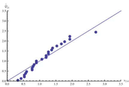
The goodness of fit for the proposed distributions ofX1andX2were ascertained by Q-Q plots, which have been obtained by plotting the pointsx1(r),Q1(ur)
(Figure 1)
and x2(r),Q21(ur|uˆ1)(Figure 2), where ur = r−n0.5, r = 1, 2, ..., 25. The value ˆu1 can be replaced by any ˆui , which satisfiesQ1(uˆi) =x1(i)to draw Figure 2. The figures indicate that the model explains the data satisfactorily.
0 10 20 30 40
x1HrL
0 10 20 30 40 Q`
1
Figure 1 –Q-Q Plot obtained by plotting(x1(r),Q1(ur)).
0.0 0.5 1.0 1.5 2.0 2.5 3.0 3.5
x2HrL
0.0 0.5 1.0 1.5 2.0 2.5 3.0 3.5 Q` 21
Figure 2 –Q-Q Plot obtained by plotting(x2(r),Q21(ur)|uˆ1).
7. CONCLUSION
in terms of bivariate quantile functions and their properties are studied. We have illus-trated how new quantile functions can be generated and used in real life data.
ACKNOWLEDGEMENTS
We thank the anonymous Referee for his/her valuable comments that enhanced the contents and presentation of the paper.
REFERENCES
K. ADAMIDIS, S. LOUKAS (1998). A lifetime distribution with decreasing failure rate. Statistics and Probability Letters, 39, pp. 35–42.
F. BELZUNCE, A. CASTANO, A. OLVERA-CERVANTES, A. SUAREZ-LLORENS(2007). Quantile curves and dependence structure of bivariate distributions. Computational Statistics and Data Analysis, 51, pp. 5112–5129.
Y. CAI(2010). Multivariate quantile function models. Statistica Sinica, 20, pp. 481–496. L. A. CHEN, A. H. WELSH(2002).Distribution function-based bivariate quantiles.
Jour-nal of Multivariate AJour-nalysis, 83, pp. 208–231.
A. M. FRANCO-PEREIRA, M. SHAKED, R. E. LILLO(2012). The decreasing percentile residual life ageing notion. Statistics, 46, pp. 587–603.
W. G. GILCHRIST(2000). Statistical Modelling with Quantile Functions. Chapman and Hall/CRC Press, Boca Raton.
J. R. M. HOSKING, J. R. WALLIS(1997).Regional Frequency Analysis: An approach based on L-moments. Cambridge University Press, Cambridge.
T. HU, B. E. KHALEDI, M. SHAKED(2003).Multivariate hazard rate ordering. Journal of Multivariate Analysis, 84, pp. 173–189.
N. L. JOHNSON, S. KOTZ(1975). A vector valued multivariate hazard rate. Journal of Multivariate Analysis, 5, pp. 53–66.
S. KAYAL, M. TRIPATHY(2018). A quantile-based tsallis-αdivergence. Physica A: Sta-tistical Mechanics and its Applications, 492, no. 15, pp. 496–505.
J. P. KLEIN, M. L. MOESCHBERGER(1997). Survival Analysis Techniques for Censored and Truncated Data. Springer, New York.
C. LIN, L. ZHANG, Y. ZHOU(2016). Quantile approach of dynamic generalized entropy (divergence) measure. Journal of Nonparametric Statistics, 28, pp. 617–643.
N. N. MIDHU, P. G. SANKARAN, N. U. NAIR(2013). A class of distributions with linear mean residual quantile function and its generalizations. Statistical Methodology, 15, pp. 1–24.
N. N. MIDHU, P. G. SANKARAN, N. U. NAIR(2014).A class of distributions with linear hazard quantile function. Communications in Statistics: Theory and Methods, 43, pp. 3674–3689.
N. U. NAIR, P. G. SANKARAN(2009).Quantile-based reliability analysis. Communica-tions in Statistics: Theory and Methods, 38, pp. 222–232.
N. U. NAIR, P. G. SANKARAN, N. BALAKRISHNAN(2013).Quantile-based Reliability Analysis. Springer- Science, New York.
N. U. NAIR, B. VINESHKUMAR(2010).L-moments of residual life. Journal of Statistical Planning and Inference, 140, pp. 2618–2631.
N. U. NAIR, B. VINESHKUMAR(2011). Ageing concepts: An approach based on quantile functions. Statistics and Probability Letters, 81, pp. 2016–2025.
F. SADEGHI, F. YOUSEFZADEH, M. CHAHKANDI(2019). Some new stochastic orders based on quantile function. Communications in Statistics- Theory and Methods, 48, no. 2, pp. 942–953.
R. SERFLING(2002).Quantile functions for multivariate analysis: Approaches and appli-cations. Statistica Neerlandica, 56, pp. 214–232.
M. SHAKED, J. G. SHANTHIKUMAR(2007).Stochastic Orders. Springer, New York. P. SONI, I. DEWAN(2012).Nonparametric estimation of quantile density function.
Com-putational Statistics and Data analysis, 56, pp. 3876–3886.
B. VINESHKUMAR, N. U. NAIR, P. G. SANKARAN (2015). Stochastic orders using quantile-based reliability functions. Journal of the Korean Statistical Society, 44, pp. 221–231.
SUMMARY
In this paper we propose a new definition of bivariate quantile function suited for reliability mod-elling and illustrate its applications. The bivariate hazard and mean residual quantile functions are defined and their properties are studied. Examples of generating new quantile functions and application of the results to model data are provided.