How Often to Sample a Continuous-Time Process in the Presence of Market Microstructure Noise

Process in the Presence of Market

Microstructure Noise

Yacine Aı¨t-Sahalia

Princeton University and NBER

Per A. Mykland

The University of Chicago

Lan Zhang

Carnegie Mellon University

In theory, the sum of squares of log returns sampled at high frequency estimates their variance. When market microstructure noise is present but unaccounted for, however, we show that the optimal sampling frequency is finite and derives its closed-form expression. But even with optimal sampling, using say 5-min returns when transac-tions are recorded every second, a vast amount of data is discarded, in contradiction to basic statistical principles. We demonstrate that modeling the noise and using all the data is a better solution, even if one misspecifies the noise distribution. So the answer is: sample as often as possible.

Over the past few years, price data sampled at very high frequency have become increasingly available in the form of the Olsen dataset of currency exchange rates or the TAQ database of NYSE stocks. If such data were not affected by market microstructure noise, the realized volatility of the process (i.e., the average sum of squares of log-returns sampled at high frequency) would estimate the returns’ variance, as is well known. In fact, sampling as often as possible would theoretically produce in the limit a perfect estimate of that variance.

We start by asking whether it remains optimal to sample the price process at very high frequency in the presence of market microstructure noise, consistently with the basic statistical principle that, ceteris paribus, more data are preferred to less. We first show that, if noise is present but unaccounted for, then the optimal sampling frequency is finite, and we

We are grateful for comments and suggestions from the editor, Maureen O’Hara, and two anonymous referees, as well as seminar participants at Berkeley, Harvard, NYU, MIT, Stanford, the Econometric Society and the Joint Statistical Meetings. Financial support from the NSF under grants SBR-0111140 (Aı¨t-Sahalia), DMS-0204639 (Mykland and Zhang), and the NIH under grant RO1 AG023141-01 (Zhang) is also gratefully acknowledged. Address correspondence to: Yacine Aı¨t-Sahalia, Bendheim Center for Finance, Princeton University, Princeton, NJ 08540, (609) 258-4015 or email: [email protected].

derive a closed-form formula for it. The intuition for this result is as follows. The volatility of the underlying efficient price process and the market microstructure noise tend to behave differently at different fre-quencies. Thinking in terms of signal-to-noise ratio, a log-return observed from transaction prices over a tiny time interval is mostly composed of market microstructure noise and brings little information regarding the volatility of the price process since the latter is (at least in the Brownian case) proportional to the time interval separating successive observations. As the time interval separating the two prices in the log-return increases, the amount of market microstructure noise remains constant, since each price is measured with error, while the informational content of volatility increases. Hence very high frequency data are mostly composed of market microstructure noise, while the volatility of the price process is more apparent in longer horizon returns. Running counter to this effect is the basic statistical principle mentioned above: in an idealized setting where the data are observed without error, sampling more frequently can be useful. What is the right balance to strike? What we show is that these two effects compensate each other and result in a finite optimal sampling frequency (in the root mean squared error sense) so that some time aggregation of the returns data is advisable.

By providing a quantitative answer to the question of how often one should sample, we hope to reduce the arbitrariness of the choices that have been made in the empirical literature using high frequency data: for example, using essentially the same Olsen exchange rate series, these somewhat ad hoc choices range from 5-min intervals [e.g., Andersen et al. (2001), Barndorff-Nielsen and Shephard (2002), Genc¸ay et al. (2002) to as long as 30 min [e.g., Andersen et al. (2003)]. When calibrating our analysis to the amount of microstructure noise that has been reported in the literature, we demonstrate how the optimal sampling interval should be determined: for instance, depending upon the amount of mi-crostructure noise relative to the variance of the underlying returns, the optimal sampling frequency varies from 4 min to 3 h, if 1 day’s worth of data are used at a time. If a longer time period is used in the analysis, then the optimal sampling frequency can be considerably longer than these values.

But even if one determines the sampling frequency optimally, the fact remains that the empirical researcher is not making full use of the data at his disposal. For instance, suppose that we have available transaction records on a liquid stock, traded once every second. Over a typical 6.5 h day, we therefore start with 23,400 observations. If one decides to sample once every 5 minutes, then — whether or not this is the optimal sampling frequency — it amounts to retaining only 78 observations. Stated differ-ently, one is throwing away 299 out of every 300 transactions. From a statistical perspective, this is unlikely to be the optimal solution, even

though it is undoubtedly better than computing a volatility estimate using noisy squared log-returns sampled every second. Somehow, an optimal solution should make use of all the data, and this is where our analysis is headed next.

So, if one decides to account for the presence of the noise, how should one proceed? We show that modeling the noise term explicitly restores the first order statistical effect that sampling as often as possible is opti-mal. This will involve an estimator different from the simple sum of squared log-returns. Since we work within a fullyparametricframework, likelihoodis the key word. Hence we construct the likelihood function for the observed log-returns, which include microstructure noise. To do so, we must postulate a model for the noise term. We assume that the noise is Gaussian. In light of what we know from the sophisticated theoretical microstructure literature, this is likely to be overly simplistic and one may well be concerned about the effect(s) of this assumption. Could it be more harmful than useful? Surprisingly, we demonstrate that our likelihood correction, based on the Gaussianity of the noise, works even if one misspecifies the assumed distribution of the noise term. Specifically, if the econometrician assumes that the noise terms are normally distributed when in fact they are not, not only is it still optimal to sample as often as possible (unlike the result when no allowance is made for the presence of noise), but the estimator has thesame varianceas if the noise distribution had been correctly specified. This robustness result is, we think, a major argument in favor of incorporating the presence of the noise when esti-mating continuous time models with high frequency financial data, even if one is unsure about the true distribution of the noise term.

In other words, the answer to the question we pose in our title is ‘‘as often as possible,’’ provided one accounts for the presence of the noise when designing the estimator (and we suggest maximum likelihood as a means of doing so). If one is unwilling to account for the noise, then one has to rely on the finite optimal sampling frequency we start our analysis with. However, we stress that while it is optimal if one insists upon using sums of squares of log-returns, this is not the best possible approach to estimate volatility given the complete high frequency dataset at hand.

In a companion paper [Zhang, Mykland, and Aı¨t-Sahalia (2003)], we study the corresponding nonparametricproblem, where the volatility of the underlying price is a stochastic process, and nothing else is known about it, in particular no parametric structure. In that case, the object of interest is the integrated volatility of the process over a fixed time interval, such as a day, and we show how to estimate it using again all the data available (instead of sparse sampling at an arbitrarily lower frequency of, say, 5 min). Since the model is nonparametric, we no longer use a likeli-hood approach but instead propose a solution based on subsampling and averaging, which involves estimators constructed on two different time

scales, and demonstrate that this again dominates sampling at a lower frequency, whether arbitrarily or optimally determined.

This article is organized as follows. We start by describing in Section 1 our reduced form setup and the underlying structural models that support it. We then review in Section 2 the base case where no noise is present, before analyzing in Section 3 the situation where the noise is ignored. In Section 4, we examine the concrete implications of this result for empirical work with high frequency data. Next, we show in Section 5 that account-ing for the presence of the noise through the likelihood restores the optimality of high frequency sampling. Our robustness results are pre-sented in Section 6 and interpreted in Section 7. In Section 8, we study the same questions when the observations are sampled at random time inter-vals, which are an essential feature of transaction-level data. We then turn to various extensions and relaxation of our assumptions in Section 9; we added a drift term, then serially correlated and cross-correlated noise respectively. In Section 10 concludes. All proofs are in the appendix.

1. Setup

Our basic setup is as follows. We assume that the underlying process of interest, typically the log-price of a security, is a time-homogeneous diffusion on the real line

dXt¼mðXt;uÞdtþsdWt, ð1Þ whereX0¼0,Wtis a Brownian motion,m(., .) is the drift function,s2the

diffusion coefficient, anduthe drift parameters, whereu 2 Qands>0. The parameter space is an open and bounded set. As usual, the restriction thatsis constant is without loss of generality since in the univariate case a one-to-one transformation can always reduce a known specifications(Xt) to that case. Also, as discussed in Aı¨t-Sahalia and Mykland (2003), the properties of parametric estimators in this model are quite different depending upon whether we estimate u alone, s2alone, or both para-meters together. When the data are noisy, the main effects that we describe are already present in the simpler of these three cases, wheres2alone is estimated, and so we focus on that case. Moreover, in the high frequency context we have in mind, the diffusive component of (1) is of order (dt)1/2 while the drift component is of orderdt only, so the drift component is mathematically negligible at high frequencies. This is validated empirical-ly: including a drift which actually deteriorates the performance of vari-ance estimates from high frequency data since the drift is estimated with a large standard error. Not centering the log returns for the purpose of variance estimation produces more accurate results [see Merton (1980)]. So we simplify the analysis one step further by settingm¼0, which we do

until Section 9.1, where we then show that adding a drift term does not alter our results. In Section 9.4, we discuss the situation where the instantaneous volatilitysis stochastic.

But for now,

Xt¼sWt: ð2Þ

Until Section 8, we treat the case where our observations occur at equi-distant time intervalsD, in which case the parameter s2is estimated at timeTon the basis ofNþ1 discrete observations recorded at timest0¼0, t1¼D,. . .,tN¼ND¼T. In Section 8, we let the sampling intervals them-selves be random variables, since this feature is an essential characteristic of high frequency transaction data.

The notion that the observed transaction price in high frequency finan-cial data is the unobservable efficient price plus some noise component due to the imperfections of the trading process is a well established concept in the market microstructure literature [see, for instance Black (1986)]. So, we depart from the inference setup previously studied [Aı¨t-Sahalia and Mykland (2003)] and we now assume that, instead of observing the processXat datesti, we observeXwith error:

~ X

Xti ¼XtiþUti, ð3Þ

where theUtis are i.i.d. noise with mean zero and variance a

2

and are independent of theWprocess. In this context, we viewXas the efficient log-price, while the observedXX~ is the transaction log-price. In an efficient market,Xtis the log of the expectation of the final value of the security conditional on all publicly available information at timet. It corresponds to the log-price that would be, in effect, in a perfect market with no trading imperfections, frictions, or informational effects. The Brownian motion Wis the process representing the arrival of new information, which in this idealized setting is immediately impounded inX.

By contrast,Utsummarizes the noise generated by the mechanics of the trading process. We view the source of noise as a diverse array of market microstructure effects, either information or non-information related, such as the presence of a bid-ask spread and the corresponding bounces, the differences in trade sizes and the corresponding differences in repre-sentativeness of the prices, the different informational content of price changes owing to informational asymmetries of traders, the gradual response of prices to a block trade, the strategic component of the order flow, inventory control effects, the discreteness of price changes in mar-kets that are not decimalized, etc., all summarized into the termU. That these phenomena are real and important and this is an accepted fact in the market microstructure literature, both theoretical and empirical. One can in fact argue that these phenomena justify this literature.

We view Equation (3) as the simplest possible reduced form of struc-tural market microstructure models. The efficient price processXis typ-ically modeled as a random walk, that is, the discrete time equivalent of Equation (2). Our specification coincides with that of Hasbrouck (1993), who discusses the theoretical market microstructure underpinnings of such a model and argues that the parameter ais a summary measure of market quality. Structural market microstructure models do generate Equation (3). For instance, Roll (1984) proposes a model whereUis due entirely to the bid-ask spread. Harris (1990b) notes that in practice there are sources of noise other than just the bid-ask spread, and studies their effect on the Roll model and its estimators.

Indeed, a disturbance U can also be generated by adverse selection effects as in Glosten (1987) and Glosten and Harris (1988), where the spread has two components: one that is owing to monopoly power, clear-ing costs, inventory carryclear-ing costs, etc., as previously, and a second one that arises because of adverse selection whereby the specialist is concerned that the investor on the other side of the transaction has superior infor-mation. When asymmetric information is involved, the disturbance U would typically no longer be uncorrelated with theWprocess and would exhibit autocorrelation at the first order, which would complicate our analysis without fundamentally altering it: see Sections 9.2 and 9.3 where we relax the assumptions that theUs are serially uncorrelated and independent of theWprocess.

The situation where the measurement error is primarily due to the fact that transaction prices are multiples of a tick size (i.e.,XX~ti ¼mikwherekis the tick size and miis the integer closest to Xti/k) can be modeled as a rounding off problem [see Gottlieb and Kalay (1985), Jacod (1996), Delattre and Jacod (1997)]. The specification of the model in Harris (1990a) combines both the rounding and bid-ask effects as the dual sources of the noise termU. Finally, structural models, such as that of Madhavan, Richardson, and Roomans (1997), also give rise to reduced forms where the observed transaction priceXX~ takes the form of an unob-served fundamental value plus error.

With Equation (3) as our basic data generating process, we now turn to the questions we address in this article: how often should one sample a continuous-time process when the data are subject to market micro-structure noise, what are the implications of the noise for the estimation of the parameters of theXprocess, and how should one correct for the presence of the noise, allowing for the possibility that the econometrician misspecifies the assumed distribution of the noise term, and finally allowing for the sampling to occur at random points in time? We pro-ceed from the simplest to the most complex situation by adding one extra layer of complexity at a time: Figure 1 shows the three sampling schemes we consider, starting with fixed sampling without market

microstructure noise, then moving to fixed sampling with noise and concluding with an analysis of the situation where transaction prices are not only subject to microstructure noise but are also recorded at random time intervals.

Figure 1

Various discrete sampling modes — no noise (Section 2), with noise (Sections 3–7) and randomly spaced with noise (Section 8)

2. The Baseline Case: No Microstructure Noise

We start by briefly reviewing what would happen in the absence of market microstructure noise, that is when a¼0. With X denoting the log-price, the first differences of the observations are the log-returns Yi¼XX~tiXX~ti1, i¼1,. . .,N. The observations Yi¼s(Wtiþ1Wti) are then i.i.d.N(0,s2D) so the likelihood function is

l s2 ¼ Nln 2 ps2D=22s2D1Y0Y, ð4Þ

where Y¼(Y1,. . .,YN)0. The maximum-likelihood estimator ofs2

coin-cides with the discrete approximation to the quadratic variation of the process ^ s s2¼ 1 T XN i¼1 Y_i2, ð5Þ

which has the following exact small sample moments:

E ss^2 ¼1 T XN i¼1 E Y _i2¼N s 2_D T ¼s 2_, var ss^2 ¼ 1 T2var XN i¼1 Y_i2 " # ¼ 1 T2 XN i¼1 varY_i2 ! ¼ N T2 2s 4_D2 ¼2s 4_D T and the following asymptotic distribution

T1=2ss^2s2!

T!1Nð0,vÞ, ð6Þ where

v¼avar ss^2 ¼DEh€ll s2 i1¼2s4D: ð7Þ

Thus selecting D as small as possible is optimal for the purpose of estimatings2.

3. When the Observations are Noisy but the Noise is Ignored

Suppose now that market microstructure noise is present but the presence of the Us is ignored when estimating s2. In other words, we use the log-likelihood function (4) even though the true structure of the observed log-returnsYis is given by an MA(1) process since

Yi¼XX~tiXX~ti1

¼XtiXti1þUtiUti1

¼sðWtiWti1Þ þUtiUti1

where the«is are uncorrelated with mean zero and varianceg2(if theUs are normally distributed, then the«is are i.i.d.). The relationship to the original parametrization (s2,a2) is given by

g21þh2¼var½ ¼Yi s2Dþ2a2, ð9Þ g2h¼covðYi,Yi1Þ ¼ a2: ð10Þ

Equivalently, the inverse change of variable is given by

g2¼1 2 2a 2_þs2_Dþq_sffiffiffiffiffiffiffiffiffiffiffiffiffiffiffiffiffiffiffiffiffiffiffiffiffiffiffiffiffiffiffiffiffi2_Dð4a2_þs2_DÞ , ð11Þ h¼ 1 2a2 2a 2_s2_Dþq_sffiffiffiffiffiffiffiffiffiffiffiffiffiffiffiffiffiffiffiffiffiffiffiffiffiffiffiffiffiffiffiffiffi2_Dð4a2_þs2_DÞ : ð12Þ

Two important properties of the log-returnsYis emerge from Equations (9) and (10). First, it is clear from Equation (9) that microstructure noise leads to spurious variance in observed log-returns,s2Dþ2a2versuss2D. This is consistent with the predictions of theoretical microstructure models. For instance, Easley and O’Hara (1992) develop a model linking the arrival of information, the timing of trades, and the resulting price process. In their model, the transaction price will be a biased representa-tion of the efficient price process, with a variance that is both overstated and heteroskedastic due to the fact that transactions (hence the recording of an observation on the process XX~) occur at intervals that are time-varying. While our specification is too simple to capture the rich joint dynamics of price and sampling times predicted by their model, het-eroskedasticity of the observed variance will also appear in our case once we allow for time variation of the sampling intervals (see Section 8). In our model, the proportion of the total return variance that is market microstructure-induced is

p¼ 2a

2

s2_Dþ2a2 ð13Þ at observation intervalD. AsDgets smaller,pgets closer to 1, so that a larger proportion of the variance in the observed log-return is driven by market microstructure frictions, and correspondingly a lesser fraction reflects the volatility of the underlying price processX.

Second, Equation (10) implies that 1<h<0, so that log-returns are (negatively) autocorrelated with first order autocorrelation

a2/(s2Dþ2a2)¼ p/2. It has been noted that market microstructure noise has the potential to explain the empirical autocorrelation of returns. For instance, in the simple Roll model,Ut¼(s/2)Qtwheresis the bid/ask

spread andQt, the order flow indicator, is a binomial variable that takes the valuesþ1 and1 with equal probability. Therefore, var[Ut]¼a2¼s2/4. Since cov(Yi,Yi1)¼ a2, the bid/ask spread can be recovered in this

model as s¼2pffiffiffiffiffiffiffir where r¼g2h is the first-order autocorrelation of returns. French and Roll (1986) proposed to adjust variance estimates to control for such autocorrelation and Harris (1990b) studied the resulting estimators. In Sias and Starks (1997), Uarises because of the strategic trading of institutional investors which is then put forward as an expla-nation for the observed serial correlation of returns. Lo and MacKinlay (1990) show that infrequent trading has implications for the variance and autocorrelations of returns. Other empirical patterns in high frequency financial data have been documented: leptokurtosis, deterministic patterns, and volatility clustering.

Our first result shows that the optimal sampling frequency is finite when noise is present but unaccounted for. The estimator ss^2 _{obtained from} maximizing the misspecified log-likelihood function (4) is quadratic in the Yis [see Equation (5)]. In order to obtain its exact (i.e., small sample) variance, we need to calculate the fourth order cumulants of theYis since

covY_i2,Y_j2 ¼2 cov Yi,Yj

2

þcum Yi,Yi,Yj,Yj

ð14Þ

(see, e.g., Section 2.3 of McCullagh (1987) for definitions and properties of the cumulants). We have the following lemma.

Lemma 1. The fourth cumulants of the log-returns are given by

cumYi,Yj,Yk,Yl

¼

2cum4½ U, if i¼j¼k¼l,

1

ð Þs i;j;k;lð Þcum4½ U, if maxði,j,k,lÞ ¼minði,j,k,lÞ þ1,

0, otherwise, 8 > < > : ð15Þ

where s(i, j, k, l) denotes the number of indices among (i, j, k, l) that are equal tomin(i, j, k, l) and U denotes a generic random variable with the common distribution of the Utis. Its fourth cumulant is denotedcum4[U]. NowUhas mean zero, so in terms of its moments

cum4½ ¼U E U4

3E U 22: ð16Þ

In the special case whereUis normally distributed, cum4[U]¼0 and as a

result of Equation (14) the fourth cumulants of the log-returns are all 0 (since Wis normal, the log-returns are also normal in that case). If the distribution of Uis binomial as in the simple bid/ask model described above, then cum4[U]¼ s4/8; since in generalswill be a tiny percentage

We can now characterize the root mean squared error

RMSE ss^2 ¼E ss^2 s22þvarss^2 1 =2

of the estimator by the following theorem.

Theorem 1. In small samples (finite T), the bias and variance of the

estimatorss^2are given by

E ss^2 s2¼2a 2 D , ð17Þ var ss^2 ¼2 s 4_D2_þ 4s2Da2þ6a4þ2 cum4½ U TD 2 2 a4þcum4½ U T2 : ð18Þ

Its RMSE has a unique minimum in D which is reached at the optimal sampling interval D¼ 2a 4_T s4 1=3 1 ffiffiffiffiffiffiffiffiffiffiffiffiffiffiffiffiffiffiffiffiffiffiffiffiffiffiffiffiffiffiffiffiffiffiffiffiffiffiffiffiffiffiffiffiffiffiffi 12 3a 4_þcum 4½ U 3 27s4_a8_T2 s 0 @ 1 A 1=3 0 B @ þ 1þ ffiffiffiffiffiffiffiffiffiffiffiffiffiffiffiffiffiffiffiffiffiffiffiffiffiffiffiffiffiffiffiffiffiffiffiffiffiffiffiffiffiffiffiffiffiffiffi 12 3a 4_þcum 4½ U 3 27s4_a8_T2 s 0 @ 1 A 1=31 C A: ð19Þ As T grows, we have D¼2 2=3_a4=3 s4=3 T 1=3_þO 1 T1=3 : ð20Þ

The trade-off between bias and variance made explicit in Equations (17) and (18) is not unlike the situation in nonparametric estimation withD1 playing the role of the bandwidth h. A lower h reduces the bias but increases the variance, and the optimal choice of h balances the two effects.

Note that these are exact small sample expressions, valid for all T. Asymptotically inT, var½ss^2 !0, and hence the RMSE of the estimator is dominated by the bias term which is independent ofT. And given the form of the bias (17), one would in fact want to select the largestDpossible to minimize the bias (as opposed to the smallest one as in the no-noise case of Section 2). The rate at which Dshould increase with T is given by Equation (20). Also, in the limit where the noise disappears (a !0 and cum4[U]!0), the optimal sampling intervalDtends to 0.

How does a small departure from a normal distribution of the micro-structure noise affect the optimal sampling frequency? The answer is that a small positive (resp. negative) departure of cum4[U] starting from the

normal value of 0 leads to an increase (resp. decrease) inD, since

D¼D_normalþ 1þ ffiffiffiffiffiffiffiffiffiffiffiffiffiffiffiffiffiffiffi 1 2a 4 T2_s4 r !2=3 1 ffiffiffiffiffiffiffiffiffiffiffiffiffiffiffiffiffiffiffi 1 2a 4 T2_s4 r !2=3 0 @ 1 A 3 21=3_a4=3_T1=3 ffiffiffiffiffiffiffiffiffiffiffiffiffiffiffiffiffiffiffi 1 2a 4 T2_s4 r s8=3 cum4½ U þOcum4½ U2 , ð21Þ

whereD_normal is the value ofDcorresponding to Cum4[U]¼0. And, of

course, the full formula (19) can be used to get the exact answer for any departure from normality instead of the comparative static one.

Another interesting asymptotic situation occurs if one attempts to use higher and higher frequency data (D!0, say sampled every minute) over a fixed time period (Tfixed, say a day). Since the expressions in Theorem 1 are exact small sample ones, they can in particular be specialized to analyze this situation. Withn¼T/D, it follows from Equations (17) and (18) that E ss^2 ¼2na 2 T þo nð Þ ¼ 2nE U 2 T þo nð Þ, ð22Þ var ss^2 ¼2n 6a 4_{þ2 cum} 4½ U T2 þo nð Þ ¼ 4nE U 4 T2 þo nð Þ ð23Þ

soðT=2nÞss^2becomes an estimator ofE[U2]¼a2whose asymptotic vari-ance is E[U4]. Note in particular that ss^2 estimates the variance of the noise, which is essentially unrelated to the object of interests2. This type of asymptotics is relevant in the stochastic volatility case we analyze in our companion paper [Zhang, Mykland, and Aı¨t-Sahalia (2003)].

Our results also have implications for the two parallel tracks that have developed in the recent financial econometrics literature dealing with discretely observed continuous-time processes. One strand of the litera-ture has argued that estimation methods should be robust to the potential issues arising in the presence of high frequency data and, consequently, be asymptotically valid without requiring that the sampling interval D separating successive observations tend to zero [see, e.g., Hansen and Scheinkman (1995), Aı¨t-Sahalia (1996), Aı¨t-Sahalia (2002)]. Another strand of the literature has dispensed with that constraint, and the asymp-totic validity of these methods requires thatDtend to zero instead of or in addition to, an increasing length of timeTover which these observations

are recorded [see, e.g., Andersen et al. (2003), Bandi and Phillips (2003), Barndorff-Nielsen and Shephard (2002)].

The first strand of literature has been informally warning about the potential dangers of using high frequency financial data without account-ing for their inherent noise [see, e.g., Aı¨t-Sahalia (1996, p. 529)], and we propose a formal modelization of that phenomenon. The implications of our analysis are most important for the second strand of the literature, which is predicated on the use of high frequency data but does not account for the presence of market microstructure noise. Our results show that the properties of estimators based on the local sample path properties of the process (such as the quadratic variation to estimates2) change dramati-cally in the presence of noise. Complementary to this are the results of Gloter and Jacod (2000) which show that the presence of even increasingly negligible noise is sufficient to adversely affect the identification ofs2. 4. Concrete Implications for Empirical Work with High Frequency Data

The clear message of Theorem 1 for empirical researchers working with high frequency financial data is that it may be optimal to sample less frequently. As discussed in the Introduction, authors have reduced their sampling frequency below that of the actual record of observations in a somewhat ad hoc fashion, with typical choices 5 min and up. Our analysis provides not only a theoretical rationale for sampling less frequently, but also gives a precise answer to the question of ‘‘how often one should sample?’’ For that purpose, we need to calibrate the parameters appearing in Theorem 1, namelys,a, cum4[U],DandT. We assume in this

calibra-tion exercise that the noise is Gaussian, in which case cum4[U]¼0.

4.1 Stocks

We use existing studies in empirical market microstructure to calibrate the parameters. One such study is Madhavan, Richardson, and Roomans (1997), who estimated on the basis of a sample of 274 NYSE stocks that approximately 60% of the total variance of price changes is attributable to market microstructure effects (they report a range of values forp from 54% in the first half hour of trading to 65% in the last half hour, see their Table 4; they also decompose this total variance into components due to discreteness, asymmetric information, transaction costs and the interac-tion between these effects). Given that their sample contains an average of 15 transactions per hour (their Table 1), we have in our framework

p¼60%, D¼1=ð157252Þ: ð24Þ

These values imply from Equation (13) that a¼0.16% if we assume a realistic value of s¼30% per year. (We do not use their reported

volatility number since they apparently averaged the variance of price changes over the 274 stocks instead of the variance of the returns. Since different stocks have different price levels, the price variances across stocks are not directly comparable. This does not affect the estimated fraction p, however, since the price level scaling factor cancels out between the numerator and the denominator.)

The magnitude of the effect is bound to vary by type of security, market and time period. Hasbrouck (1993) estimates the value ofato be 0.33%. Some authors have reported even larger effects. Using a sample of NAS-DAQ stocks, Kaul and Nimalendran (1990) estimate that about 50% of the daily variance of returns is due to the bid-ask effect. With s¼40% (NASDAQ stocks have higher volatility), the values

p¼50%, D¼1=252

Table 1

Optimal sampling frequency

T

Value ofa 1 day 1 year 5 years

(a)s¼30% Stocks

0.01% 1 min 4 min 6 min

0.05% 5 min 31 min 53 min

0.1% 12 min 1.3 h 2.2 h 0.15% 22 min 2.2 h 3.8 h 0.2% 32 min 3.3 h 5.6 h 0.3% 57 min 5.6 h 1.5 day 0.4% 1.4 h 1.3 day 2.2 days 0.5% 2 h 1.7 day 2.9 days 0.6% 2.6 h 2.2 days 3.7 days 0.7% 3.3 h 2.7 days 4.6 days 0.8% 4.1 h 3.2 days 1.1 week 0.9% 4.9 h 3.8 days 1.3 week 1.0% 5.9 h 4.3 days 1.5 week (b)s¼10% Currencies

0.005% 4 min 23 min 39 min

0.01% 9 min 58 min 1.6 h

0.02% 23 min 2.4 h 4.1 h

0.05% 1.3 h 8.2 h 14.0 h

0.10% 3.5 h 20.7 h 1.5 day

This table reports the optimal sampling frequencyDgiven in Equation 19 for different values of the standard deviation of the noise termaand the length of the sampleT. Throughout the table, the noise is assumed to be normally distributed (hence cum4[U]¼0 in formula 19). In panel (a), the standard

deviation of the efficient price process iss¼30% per year, and ats¼10% per year in panel (b). In both panels, 1 year¼252 days, but in panel (a), 1 day¼6.5 hours (both the NYSE and NASDAQ are open for 6.5 h from 9:30 to 16:00 EST), while in panel (b), 1 day¼24 hours as is the case for major currencies. A value ofa¼0.05% means that each transaction is subject to Gaussian noise with mean 0 and standard deviation equal to 0.05% of the efficient price. If the sole source of the noise were a bid/ask spread of sizes, thenashould be set tos/2. For example, a bid/ask spread of 10 cents on a$10 stock would correspond to

a¼0.05%. For the dollar/euro exchange rate, a bid/ask spread ofs¼0.04% translates intoa¼0.02%. For the bid/ask model, which is based on binomial instead of Gaussian noise, cum4[U]¼ s4/8, but this

yield the value a¼1.8%. Also on NASDAQ, Conrad, Kaul and Nimalendran (1991) estimate that 11% of the variance of weekly returns (see their Table 4, middle portfolio) is due to bid-ask effects. The values

p¼11%, D¼1=52 imply thata¼1.4%.

In Table 1, we compute the value of the optimal sampling intervalD implied by different combinations of sample length (T) and noise magni-tude (a). The volatility of the efficient price process is held fixed at

s¼30% in Panel (A), which is a realistic value for stocks. The numbers in the table show that the optimal sampling frequency can be substantially affected by even relatively small quantities of microstructure noise. For instance, using the value a¼0.15% calibrated from Madhavan, Richardson, and Roomans (1997), we find an optimal sampling interval of 22 minutes if the sampling length is 1 day; longer sample lengths lead to higher optimal sampling intervals. With the higher value of a¼0.3%, approximating the estimate from Hasbrouck (1993), the optimal sampling interval is 57 min. A lower value of the magnitude of the noise translates into a higher frequency: for instance, D¼5 min if a¼0.05% and T¼1 day. Figure 2 displays the RMSE of the estimator as a function of D and T, using parameter values s¼30% and a¼0.15%. The figure illustrates the fact that deviations from the optimal choice ofDlead to a substantial increase in the RMSE: for example, with T¼1 month, the RMSE more than doubles if, instead of the optimal D¼1 h, one uses D¼15 min.

Figure 2

4.2 Currencies

Looking now at foreign exchange markets, empirical market microstruc-ture studies have quantified the magnitude of the bid-ask spread. For example, Bessembinder (1994) computes the average bid/ask spreadsin the wholesale market for different currencies and reports values of s ¼0.05% for the German mark, and 0.06% for the Japanese yen (see Panel B of his Table 2). We calculated the corresponding numbers for the 1996–2002 period to be 0.04% for the mark (followed by the euro) and 0.06% for the yen. Emerging market currencies have higher spreads: for instance, s¼0.12% for Korea and 0.10% for Brazil. During the same period, the volatility of the exchange rate was s¼10% for the German mark, 12% for the Japanese yen, 17% for Brazil and 18% for Korea. In Panel B of Table 1, we computeDwiths¼10%, a realistic value for the euro and yen. As we noted above, if the sole source of the noise were a bid/ ask spread of sizes, thenashould be set tos/2. Therefore, PanelBreports the values ofDfor values ofaranging from 0.02% to 0.1%. For example, the dollar/euro or dollar/yen exchange rates (calibrated to s ¼ 10%, a ¼0.02%) should be sampled everyD¼23 min if the overall sample length isT¼1 day, and every 1.1 h ifT¼1 year.

Furthermore, using the bid/ask spread alone as a proxy for all micro-structure frictions will lead, except in unusual circumstances, to an under-statement of the parametera, since variances are additive. Thus, sinceDis increasing ina, one should interpret the value ofDread off 1 on the row corresponding to a ¼ s/2 as a lower bound for the optimal sampling interval.

4.3 Monte Carlo Evidence

To validate empirically these results, we perform Monte Carlo simula-tions. We simulateM¼10,000 samples of lengthT¼1 year of the process X, add microstructure noiseUto generate the observationsXX~, and then

Table 2

Monte Carlo simulations: bias and variance when market microstructure noise is ignored

Sampling interval Theoretical mean Sample mean Theoretical stand. dev. Sample stand. dev.

5 min 0.185256 0.185254 0.00192 0.00191 15 min 0.121752 0.121749 0.00208 0.00209 30 min 0.10588 0.10589 0.00253 0.00254 1 h 0.097938 0.097943 0.00330 0.00331 2 h 0.09397 0.09401 0.00448 0.00440 1 day 0.09113 0.09115 0.00812 0.00811 1 week 0.0902 0.0907 0.0177 0.0176

This table reports the results ofM¼10,000 Monte Carlo simulations of the estimatorss^2_{, with market} microstructure noise present but ignored. The column ‘‘theoretical mean’’ reports the expected value of the estimator, as given in Equation (17) and similarly for the column ‘‘theoretical standard deviation’’ (the variance is given in Equation (18)). The ‘‘sample’’ columns report the corresponding moments computed over theMsimulated paths. The parameter values used to generate the simulated data ares2¼0.32

¼0.09

anda2 ¼(0.15%)2

the log returnsY. We sample the log-returns at various intervalsDranging from 5 min to 1 week, and calculate the bias and variance of the estimator ^

s

s2 over the M simulated paths. We then compare the results to the theoretical values given in Equations (17) and (18) of Theorem 1. The noise distribution is Gaussian, s ¼ 30% and a ¼ 0.15% — the values we calibrated to stock returns data above. Table 2 shows that the theo-retical values are in close agreement with the results of the Monte Carlo simulations.

Table 2 also illustrates the magnitude of the bias inherent in sampling at too high a frequency. While the value ofs2used to generate the data is 0.09, the expected value of the estimator when sampling every 5 min is 0.18, so on average the estimated quadratic variation is twice as big as it should be in this case.

5. Incorporating Market Microstructure Noise Explicitly

So far we have stuck to the sum of squares of log-returns as our estimator of volatility. We then showed that, for this estimator, the optimal sam-pling frequency is finite. However, this implies that one is discarding a large proportion of the high frequency sample (299 out of every 300 observations in the example described in the introduction), in order to mitigate the bias induced by market microstructure noise. Next, we show that if we explicitly incorporate theUs into the likelihood function, then we are back in a situation where the optimal sampling scheme consists in sampling as often as possible — that is, using all the data available.

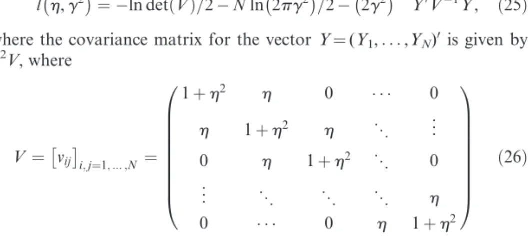
Specifying the likelihood function of the log-returns, while recognizing that they incorporate noise, requires that we take a stand on the distribu-tion of the noise term. Suppose for now that the microstructure noise is normally distributed, an assumption whose effect we will investigate below in Section 6. Under this assumption, the likelihood function for theYs is given by

lh,g2¼ ln detð ÞV =2Nln 2 pg2=22g21Y0V1Y, ð25Þ

where the covariance matrix for the vectorY¼(Y1,. . .,YN)0 is given by g2V, where V ¼ vij _i;j¼1;...;N ¼ 1þh2 h 0 0 h 1þh2 _h » .. . 0 h 1þh2 » 0 .. . » » » h 0 0 h 1þh2 0 B B B B B B B B @ 1 C C C C C C C C A ð26Þ

Further,

detð Þ ¼V 1h

2Nþ2

1h2 ð27Þ

and, neglecting the end effects, an approximate inverse ofVis the matrix V¼[vij]i,j¼1,. . .,Nwhere

vij¼ 1h2

1

h ð Þjijj

[see Durbin (1959)]. The productVVdiffers from the identity matrix only on the first and last rows. The exact inverse isV1¼[vij]i,j¼1,. . .,Nwhere vij¼1h211h2Nþ21nðhÞjijj hð Þiþj hð Þ2Nijþ2

h

ð Þ2Nþjijjþ2þ ð hÞ2Nþijþ2þ ð hÞ2Niþjþ2o ð28Þ

[see Shaman (1969), Haddad (1995)].

From the perspective of practical implementation, this estimator is nothing else than the MLE estimator of an MA(1) process with Gaussian errors: any existing computer routines for the MA(1) situation can, there-fore, be applied [see e.g., Hamilton (1995, Section 5.4)]. In particular, the likelihood function can be expressed in a computationally efficient form by triangularizing the matrixV, yielding the equivalent expression:

lh,g2¼ 1 2 XN i¼1 ln 2ð pdiÞ 1 2 XN i¼1 ~ Y Y2 i di , ð29Þ where di¼g2 1þh2_{þ þh}2i 1þh2_{þ þh}2ði1Þ

and theYYi~s are obtained recursively asYY~1¼Y1and fori¼2,. . .,N:

~ Y

Yi¼Yi

h1þh2þ þh2ði2Þ

1þh2_{þ þh}2ði1Þ YY~i1:

This latter form of the log-likelihood function involves only single sums as opposed to double sums if one were to compute Y0_V1_{Yby brute force}

using the expression ofV1given above.

We now compute the distribution of the MLE estimators ofs2anda2, which follows by the delta method from the classical result for the MA(1) estimators ofgandhby the following proposition.

Proposition 1. When U is normally distributed, the MLE ðss^2_,^aa2_{Þ is}

consistent and its asymptotic variance is given by avarnormalss^2,^aa2 ¼ 4pffiffiffiffiffiffiffiffiffiffiffiffiffiffiffiffiffiffiffiffiffiffiffiffiffiffiffiffiffiffiffiffiffis6_Dð4a2_þs2_DÞþ2s4_{D s}2_DhD,s2_,a2 D 2 2a 2_þs2_D hD,s2,a2 0 @ 1 A, with hD,s2,a2 2a2þqffiffiffiffiffiffiffiffiffiffiffiffiffiffiffiffiffiffiffiffiffiffiffiffiffiffiffiffiffiffiffiffiffis2_Dð4a2_þs2_DÞþs2_{D: ð30Þ} Since avarnormalðss^2Þis increasing inD, it is optimal to sample as often as possible. Further, since

avarnormal ss^2 ¼8s3aD1=2þ2s4Dþoð ÞD , ð31Þ

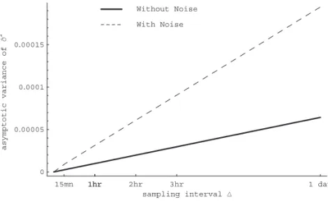
the loss of efficiency relative to the case where no market microstructure noise is present (and, ifa2¼0 is not estimated, avarðss^2Þ ¼2s4Das given in Equation (7), or ifa2¼0 is estimated, avar(s)¼6ss^4d) is at orderD1/2. Figure 3 plots the asymptotic variances ofss^2as functions ofDwith and without noise (the parameter values are again s¼30% anda¼0.15%). Figure 4 reports histograms of the distributions ofss^2and^aa2_{from 10,000} Monte Carlo simulations with the solid curve plotting the asymptotic distribution of the estimator from Proposition 1. The sample path is of lengthT¼1 year, the parameter values are the same as above, and the

Figure 3

process is sampled every 5 min — since we are now accounting explicitly for the presence of noise, there is no longer a reason to sample at lower frequencies. Indeed, the figure documents the absence of bias and the good agreement of the asymptotic distribution with the small sample one.

6. The Effect of Misspecifying the Distribution of the Microstructure Noise

We now study a situation where one attempts to incorporate the presence of the Us into the analysis, as in Section 5, but mistakenly assumes a

Figure 4

misspecified model for them. Specifically, we consider the case where the Us are assumed to be normally distributed when in reality they have a different distribution. We still suppose that theUs are i.i.d. with mean zero and variancea2.

Since the econometrician assumes theUs to have a normal distribution, inference is still done with the log-likelihood l(s2,a2), or equivalently l(h,g2) given in Equation (25), using Equations (9) and (10). This means that the scores_lls2 andll__a2, or equivalently Equations (C.1) and (C.2) are

used as moment functions (or ‘‘estimating equations’’). Since the first order moments of the moment functions only depend on the second order moment structure of the log-returns (Y1,. . .,YN), which is

unchanged by the absence of normality, the moment functions are unbi-ased under the true distribution of theUs:

Etrue _llh

h i

¼Etrue _llg2 h i

¼0 ð32Þ

and similarly forll_s2 and_ll_a2. Hence the estimatorðss^2,^aa2Þbased on these

moment functions is consistent and asymptotically unbiased (even though the likelihood function is misspecified).

The effect of misspecification, therefore, lies in the asymptotic variance matrix. By using the cumulants of the distribution ofU, we express the asymptotic variance of these estimators in terms of deviations from nor-mality. But as far as computing the actual estimator, nothing has changed relative to Section 5: we are still calculating the MLE for an MA(1) process with Gaussian errors and can apply exactly the same computa-tional routine.

However, since the error distribution is potentially misspecified, one could expect the asymptotic distribution of the estimator to be altered. This does not happen, as far asss^2_{is concerned: see the following theorem.}

Theorem 2. The estimators ðss^2_,^aa2_{Þobtained by maximizing the possibly}

misspecified log-likelihood function (25) are consistent and their asymptotic variance is given by

avartruess^2,aa^2¼avarnormalss^2,^aa2þcum4½ U

0 0

0 D

, ð33Þ

where avarnormalðss^2,^aa2Þ is the asymptotic variance in the case where the

distribution of U is normal, that is, the expression given in Proposition 1. In other words, the asymptotic variance ofss^2is identical to its expression if the Us had been normal. Therefore, the correction we proposed for the presence of market microstructure noise relying on the assumption that the noise is Gaussian is robust to misspecification of the error distribution.

Documenting the presence of the correction term through simulations presents a challenge. At the parameter values calibrated to be realistic, the order of magnitude ofais a few basis points, saya¼0.10%¼103. But if Uif of order 103, cum4[U] which is of the same order asU4, is of order

1012. In other words, with a typical noise distribution, the correction term in Equation (33) will not be visible.

Nevertheless, to make it discernible, we use a distribution forUwith the same calibrated standard deviationaas before, but a disproportionately large fourth cumulant. Such a distribution can be constructed by letting U¼vTnwherev>0 is constant andTnis a Studenttdistribution withv degrees of freedom.Tnhas mean zero, finite variance as long asv>2 and finite fourth moment (hence finite fourth cumulant) as long asv>4. But asvapproaches 4 from above,E½T4

ntends to infinity. This allows us to

produce an arbitrarily high value of cum4[U] while controlling for the

magnitude of the variance. The specific expressions ofa2and cum4[U] for

this choice ofUare given by

a2 ¼var½ ¼U v 2_n n2, ð34Þ cum4½ ¼U 6v4_n2 n4 ð Þðn2Þ2: ð35Þ

Thus, we can select the two parameters (v,n) to produce desired values of (a2, cum4[U]). As before, we set a¼0.15%. Then, given the form of the

asymptotic variance matrix Equation (33), we set cum4[U] so that

cum4½UD¼avarnormalðaa^2Þ=2. This makes avartrueð^aa2Þ by construction 50% larger than avarnormalð^aa2Þ. The resulting values of (v,n) from solving Equations (34) and (35) arev¼0.00115 andv¼4.854. As above, we set the other parameters tos¼30%,T¼1 year, andD¼5 minutes. Figure 5 reports histograms of the distributions ofss^2 _and^aa2 _{from 10,000 Monte} Carlo simulations. The solid curve plots the asymptotic distribution of the estimator, given now by Equation (33). There is again good adequacy between the asymptotic and small sample distributions. In particular, we note that as predicted by Theorem 2, the asymptotic variance of ss^2 is unchanged relative to Figure 4 while that of ^aa2 _{is 50% larger. The small} sample distribution of ss^2 appears unaffected by the non-Gaussianity of the noise; with a skewness of 0.07 and a kurtosis of 2.95, it is closely approximated by its asymptotic Gaussian limit. The small sample distri-bution of^aa2_{does exhibit some kurtosis (4.83), although not large relative} to that of the underlying noise distribution (the values ofvandnimply a kurtosis forUof 3þ6/(n4)¼10). Similar simulations but with a longer time span ofT¼5 years are even closer to the Gaussian asymptotic limit: the kurtosis of the small sample distribution of^aa2_{goes down to 2.99.}

7. Robustness to Misspecification of the Noise Distribution

Going back to the theoretical aspects, the above Theorem 2 has implica-tions for the use of the Gaussian likelihoodlthat go beyond consistency, namely that this likelihood can also be used to estimate the distribution of ^

s

s2 under misspecification. With l denoting the log-likelihood assuming that theUs are Gaussian, given in Equation (25),€llðss^2,^aa2_{Þdenote the} observed information matrix in the original parameterss2anda2. Then

^ V

V¼avaravardnormal¼ 1 T

€_llss^2_,^aa2

1

Figure 5

is the usual estimate of asymptotic variance when the distribution is correctly specified as Gaussian. Also note, however, that otherwise, so long asðss^2,aa^2Þis consistent,VV^ is also a consistent estimate of the matrix avarnormalðss^2,^aa2Þ. Since this matrix coincides with avartrueðss^2,^aa2Þfor all but the (a2, a2) term (see Equation (33)), the asymptotic variance of T1=2_ðss^2_s2_{Þis consistently estimated byVV}^

s2_s2. The similar statement is

true for the covariances, but not, obviously, for the asymptotic variance of T1=2_ð^aa2_a2_Þ.

In the likelihood context, the possibility of estimating the asymptotic variance by the observed information is due to the second Bartlett iden-tity. For a general log likelihoodl, ifS Etrue½_ll_ll0=NandD Etrue½€ll=N (differentiation refers to the original parameters (s2,a2), not the trans-formed parameters (g2,h)) this identity says that

SD¼0: ð36Þ

It implies that the asymptotic variance takes the form

avar¼DDS1D1¼DD1: ð37Þ

It is clear that Equation (37) remains valid if the second Bartlett identity holds only to first order, that is,

SD¼oð Þ1 ð38Þ

asN! 1, for a general criterion functionlwhich satisfiesEtrue½ll_ ¼oðNÞ. However, in view of Theorem 2, Equation (38) cannot be satisfied. In fact, we show in Appendix E that

SD¼cum4½ Ugg0þoð Þ1 , ð39Þ where g¼ gs2 g_a2 ¼ D1=2 s_ð4a2_þs2_DÞ3=2 1 2a4 1 D1=2_s 6a2_þs2_D ð Þ 4a2_þs2_D ð Þ3=2 0 B B @ 1 C C A: ð40Þ

From Equation (40), we see thatg 6¼ 0 whenevers2>0. This is consistent with the result in Theorem 2 that the true asymptotic variance matrix, avartrueðss^2,^aa2Þ; does not coincide with the one for Gaussian noise, avarnormalðss^2,aa^2Þ. On the other hand, the 22 matrixgg0 is of rank 1, signaling that there exist linear combinations that will cancel out the first column ofSD. From what we already know of the form of the correc-tion matrix,D1gives such a combination that the asymptotic variance of the original parameters (s2,a2) will have the property that its first column is not subject to correction in the absence of normality.

A curious consequence of Equation (39) is that while the observed information can be used to estimate the asymptotic variance ofss^2_when

a2is not known, this is not the case whena2is known. This is because the second Bartlett identity also fails to first order when considering a2 to be known, that is, when differentiating with respect tos2only. Indeed, in that case we have from the upper left component in the matrix Equation (39): Ss2_s2D_s2_s2¼N1E_true i_s2_s2s2,a22 h i þN1Etrue €lls2_s2s2,a2 h i ¼cum4½ ÞU ðgs2Þ2þoð Þ1 ,

which is noto(1) unless cum4[U]¼0.

To make the connection between Theorem 2 and the second Bartlett identity, one needs to go to the log profile likelihood

l s2 sup a2

ls2,a2: ð41Þ

Obviously, maximizing the likelihoodl(s2,a2) is the same as maximizing

l(s2). Thus one can think ofs2as being estimated (whena2is unknown) by maximizing the criterion functionl(s2), or by solvingllð_ ss^2_{Þ ¼0. Also,} the observed profile information is related to the original observed information by

€

l

l ss^2 1¼h€llss^2,^aa21i

s2_s2, ð42Þ

that is, the first (upper left hand corner) component of the inverse observed information in the original problem. We explain this in Appendix E, where we also show thatEtrue½ll ¼_ oðNÞ. In view of Theorem 2,€llðss^2_{Þcan be used to estimate the asymptotic variance ofss^}2 _{under the} true (possibly non-Gaussian) distribution of theUs, and so it must be that the criterion functionlsatisfies Equation (38), that is

N1Etrue ll s_ 22

h i

þN1Etruell s€ 2 ¼oð Þ1 : ð43Þ This is indeed the case, as shown in Appendix E.

This phenomenon is related, although not identical, to what occurs in the context of likelihood [for comprehensive treatments of quasi-likelihood theory, see the books by McCullagh and Nelder (1989) and Heyde (1997), and the references therein, and for early econometrics examples, see Macurdy (1982) and White (1982)]. In quasi-likelihood situations, one uses a possibly incorrectly specified score vector which is

nevertheless required to satisfy the second Bartlett identity. What makes our situation unusual relative to quasi-likelihood is that the interest parameter s2and the nuisance parameter a2 are entangled in the same estimating equations (ll_s2 andll__a2 from the Gaussian likelihood) in such a

way that the estimate ofs2depends, to first order, on whethera2is known or not. This is unlike the typical development of quasi-likelihood, where the nuisance parameter separates out [see, e.g., McCullagh and Nelder (1989, Table 9.1, p. 326)]. Thus only by going to the profile likelihoodl

can one make the usual comparison to quasi-likelihood.

8. Randomly Spaced Sampling Intervals

One essential feature of transaction data in finance is that the time that separates successive observations is random, or at least time-varying. So, as in Aı¨t-Sahalia and Mykland (2003), we are led to consider the case whereDi¼titi1are either deterministic and time-varying, or random

in which case we assume for simplicity that they are i.i.d., independent of theWprocess. This assumption, while not completely realistic [see Engle and Russell (1998) for a discrete time analysis of the autoregressive dependence of the times between trades] allows us to make explicit calcu-lations at the interface between the continuous and discrete time scales. We denote byNTthe number of observations recorded by timeT.NT is random if theDs are. We also suppose thatUtican be writtenUi, where the Ui are i.i.d. and independent of the W process and the Dis. Thus, the observation noise is the same at all observation times, whether random or nonrandom. If we define the Yis as before, in the first two lines of Equation (8), though the MA(1) representation is not valid in the same form.

We can do inference conditionally on the observed sampling times, in light of the fact that the likelihood function using all the available infor-mation is

L YNð ,DN,. . .,Y1,D1;b,cÞ ¼L YNð ,. . .,Y1jDN,. . .,D1;bÞ

LðDN,. . .,D1;cÞ,

wherebare the parameters of the state process, that is (s2,a2), andcare the parameters of the sampling process, if any (the density of the sampling intervals densityL(DNT,. . .,D1;c) may have its own nuisance parameters

c, such as an unknown arrival rate, but we assume that it does not depend on the parameters b of the state process). The corresponding log-likelihood function is XN n¼1 lnL Yð N,. . .,Y1jDN,. . .,D1;bÞ þ X N1 n¼1 lnLðDN,. . .,D1;cÞ ð44Þ

and since we only care aboutb, we only need to maximize the first term in that sum.

We operate on the covariance matrix of the log-returns Ys, now given by ¼ s2_D 1þ2a2 a2 0 0 a2 s2D2þ2a2 a2 » .. . 0 a2 s2D3þ2a2 » 0 .. . » » » a2 0 0 a2 _s2_D nþ2a2 0 B B B B B B B B B @ 1 C C C C C C C C C A : ð45Þ

Note that in the equally spaced case, ¼g2V. But now Y no longer follows an MA(1) process in general. Furthermore, the time variation in Dis gives rise to heteroskedasticity as is clear from the diagonal elements of . This is consistent with the predictions of the model of Easley and O’Hara (1992) where the variance of the transaction price processXX~ is heteroskedastic as a result of the influence of the sampling times. In their model, the sampling times are autocorrelated and correlated with the evolution of the price process, factors we have assumed away here. However, Aı¨t-Sahalia and Mykland (2003) show how to conduct likeli-hood inference in such a situation.

The log-likelihood function is given by lnL Yð N,. . .,Y1jDN,. . . ,D1;bÞ

ls2,a2¼ ln detð Þ =2Nln 2ð pÞ=2Y01Y=2: ð46Þ

In order to calculate this log-likelihood function in a computationally efficient manner, it is desirable to avoid the ‘‘brute force’’ inversion of theNNmatrix. We extend the method used in the MA(1) case (see Equation (29)) as follows. By Theorem 5.3.1 in Dahlquist and Bjoorck€ (1974), and the development in the proof of their Theorem 5.4.3, we can decomposein the form¼LDLT, whereLis a lower triangular matrix whose diagonals are all 1 and D is diagonal. To compute the rele-vant quantities, their Example 5.4.3 shows that if one writes D ¼

diag(g1,. . .,gn) and L¼ 1 0 0 0 k2 1 0 » .. . 0 k3 1 » 0 .. . » » » 0 0 0 kn 1 0 B B B B B B B @ 1 C C C C C C C A , ð47Þ

then thegksandkksfollow the recursion equationg1¼s2D1þ2a2and for

i¼2,. . .,N:

ki¼ a2=gi1 and gi¼s2Diþ2a2þkia2: ð48Þ Then, define YY~ ¼L1_{Y so that Y}01_{Y ¼YY~}0_D1_YY~_{. From Y ¼LYY}~_{, it} follows thatYY~1¼Y1and, fori¼2,. . .,N:

~ Y

Yi¼YikiYY~i1:

And det()¼det(D) since det(L)¼1. Thus we have obtained a computa-tionally simple form for Equation (46) that generalizes the MA(1) form in Equation (29) to the case of non-identical sampling intervals:

ls2,a2_¼ 1 2 XN i¼1 ln 2ð pgiÞ 1 2 XN i¼1 ~ Y Y2 i gi : ð49Þ

We can now turn to statistical inference using this likelihood function. As usual, the asymptotic variance ofT1=2_ðss^2_s2_,^aa2_a2_{Þis of the form}

avarss^2,^aa2¼ lim T! 1 1 TE €_ll s2_s2 h i 1 TE €_ll s2_a2 h i 1 TE €_ll a2_a2 h i 0 B @ 1 C A 1 : ð50Þ

To compute this quantity, suppose in the following that b1and b2can

represent eithers2ora2. We start with:

Lemma 2. Fisher’s Conditional Information is given by

E €llb₂b₁ D h i ¼ 1 2 q2ln det qb₂b₁ : ð51Þ

To compute the asymptotic distribution of the MLE of (b1,b2), one would

then need to compute the inverse ofE½€llb₂b₁ ¼ED½E½€llb₂b₁jDwhereED denotes expectation taken over the law of the sampling intervals. From Equation (51), and since the order of ED and q2/qb2b1 can be

inter-changed, this requires the computation of

ED½ln det ¼ED½ln detD ¼

XN

i¼1

ED½lnð Þgi ,

where from Equation (48) thegis are given by the continuous fraction

g1¼s2D1þ2a2, g2¼s2D2þ2a2 a4 s2_D 1þ2a2 , g3¼s2D3þ2a2 a4 s2_D 2þ2a2 a4 s2_D 1þ2a2

and in general gi¼s2Diþ2a2 a4 s2_D i1þ2a2 a4 »

It, therefore, appears that computing the expected value of ln(gi) over the law of (D1,D2,. . .,Di) will be impractical.

8.1 Expansion around a fixed value ofD

To continue further with the calculations, we propose to expand around a fixed value ofD, namelyD0¼E[D]. Specifically, suppose now that

Di¼D0ð1þejiÞ, ð52Þ

whereeandD0are nonrandom, the jis are i.i.d. random variables with mean zero and finite distribution. We will Taylor-expand the expressions above around e¼0, that is, around the non-random sampling case we have just finished dealing with. Our expansion is one that is valid when the randomness of the sampling intervals remains small, that is, when var[Di] is small, oro(1). Then we haveD0¼E[D]¼O(1) and var½Di ¼D20e2var½ji. The natural scaling is to make the distribution of ji finite, that is, var[ji]¼O(1), so thate2¼O(var[Di])¼o(1). But any other choice would have no impact on the result since var[Di]¼o(1) implies that the product

e2var[ji] iso(1) and whenever we write remainder terms below they can be expressed asOp(e3j3) instead of justO(e3). We keep the latter notation for clarity given that we setji¼Op(1). Furthermore, for simplicity, we take thejis to be bounded.

We emphasize that the time increments or durationsDido not tend to zero length ase!0. It is only the variability of theDis that goes to zero. Denote by0the value ofwhenDis replaced byD0, and letXdenote

the matrix whose diagonal elements are the terms D0ji, and whose off-diagonal elements are zero. We obtain the following theorem.

Theorem 3. The MLEðss^2_,^aa2_{Þis again consistent, this time with asymptotic}

variance avarss^2,^aa2¼Að Þ0 þe2Að Þ2 þO e3 , ð53Þ where Að Þ0 ¼ 4 ffiffiffiffiffiffiffiffiffiffiffiffiffiffiffiffiffiffiffiffiffiffiffiffiffiffiffiffiffiffiffiffiffiffiffiffis6_D 0ð4a2þs2D0Þ p þ2s4_D 0 s2D0hD0,s2,a2 D0 2 2a 2_þs2_D 0 hD0,s2,a2 0 @ 1 A

and Að Þ2 ¼ var½ j 4a2_þD 0s2 ð Þ Að Þ_s22_s2 A 2 ð Þ s2_a2 Að Þ_a22_a2 ! with Að_s22Þ_s2¼ 4ðD 2 0s6þD 3=2 0 s5 ffiffiffiffiffiffiffiffiffiffiffiffiffiffiffiffiffiffiffiffiffiffiffi 4a2_þD 0s2 p Þ, Að_s22Þ_a2¼D 3=2 0 s 3 ffiffiffiffiffiffiffiffiffiffiffiffiffiffiffiffiffiffiffiffiffiffiffi_4a2_þD 0s2 p ð2a2þ3D₀s2Þ þD2₀s4ð8a2þ3D₀s2Þ, Að_a22Þ_a2¼ D 2 0s2ð2a2þs ffiffiffiffiffiffi D0 p ffiffiffiffiffiffiffiffiffiffiffiffiffiffiffiffiffiffiffiffiffiffiffi 4a2_þD 0s2 p þD0s2Þ2:

In connection with the preceding result, we underline that the quantity avarðss^2_,^aa2_{Þ is a limit as T ! 1, as in Equation (50). Equation (53),} therefore, is an expansion ineafterT! 1.

Note that A(0) is the asymptotic variance matrix already present in Proposition 1, except that it is evaluated atD0=E[D]. Note also that the

second order correction term is proportional to var[j], and is therefore zero in the absence of sampling randomness. When that happens,D¼D0

with probability one and the asymptotic variance of the estimator reduces to the leading term A(0), that is, to the result in the fixed sampling case given in Proposition 1.

8.2 Randomly spaced sampling intervals and misspecified microstructure noise

Suppose now, as in Section 6, that theUs are i.i.d., have mean zero and variance a2, but are otherwise not necessarily Gaussian. We adopt the same approach as in Section 6, namely to express the estimator’s proper-ties in terms of deviations from the deterministic and Gaussian case. The additional correction terms in the asymptotic variance are given in the following result.

Theorem 4. The asymptotic variance is given by

avartruess^,^aa2¼ Að Þ0 þcum4½ UBð Þ0

þe2 Að Þ2 þcum4½ UBð Þ2

þO e3 ð54Þ

where A(0)andA(2)are given in the statement of Theorem 3 and Bð Þ0 ¼ 0 0

0 D₀

while Bð Þ2 ¼var½ j B 2 ð Þ s2_s2 B 2 ð Þ s2_a2 Bð Þ_a22_a2 ! Bð Þ_s22_s2¼ 10D3₀=2s5 4a2_þD 0s2 ð Þ5=2þ 4D2₀s6 _16a4_þ11a2_D 0s2þ2D20s4 2a2_þD 0s2 ð Þ3 4a2_þD 0s2 ð Þ2 Bð Þ_s22_a2 ¼ D2₀s4 2a2_þD 0s2 ð Þ3 4a2_þD 0s2 ð Þ5=2 ffiffiffiffiffiffiffiffiffiffiffiffiffiffiffiffiffiffiffiffiffiffiffi4a2_þD 0s2 p 32a6þ64a4D0s2þ35a2D20s4þ6D 3 0s6 þD1₀=2s 116a6þ126a4D0s2þ47a2D20s 4_þ6D3 0s 6 Bð Þ_a22_a2¼ 16a8_D5=2 0 s3 13a4þ10a2D0s2þ2D20s4 2a2_þD 0s2 ð Þ3 4a2_þD 0s2 ð Þ5=22a2_þs2_Dp_sffiffiffiffiffiffiffiffiffiffiffiffiffiffiffiffiffiffiffiffiffiffiffiffiffiffiffiffiffiffiffiffiffi2_Dð4a2_þs2_DÞ 2 :

The termA(0) is the base asymptotic variance of the estimator, already present with fixed sampling and Gaussian noise. The term cum4[U]B(0)is

the correction due to the misspecification of the error distribution. These two terms are identical to those present in Theorem 2. The terms propor-tional toe2are the further correction terms introduced by the randomness of the sampling. A(2) is the base correction term present even with Gaussian noise in Theorem 3, and cum4[U]B(2)is the further correction

due to the sampling randomness. Both A(2) andB(2) are proportionalto var[j] and hence vanish in the absence of sampling randomness.

9. Extensions

In this section, we briefly sketch four extensions of our basic model. First, we show that the introduction of a drift term does not alter our conclu-sions. Then we examine the situation where market microstructure noise is serially correlated; there, we show that the insight of Theorem 1 remains valid, namely that the optimal sampling frequency is finite. Third, we turn to the case where the noise is correlated with the efficient price signal. Fourth, we discuss what happens if volatility is stochastic.

In a nutshell, each one of these assumptions can be relaxed without affecting our main conclusion, namely that the presence of the noise gives rise to a finite optimal sampling frequency. The second part of our anal-ysis, dealing with likelihood corrections for microstructure noise, will not

necessarily carry through unchanged if the assumptions are relaxed (for instance, there is not even a known likelihood function if volatility is stochastic, and the likelihood must be modified if the assumed variance-covariance structure of the noise is modified).

9.1 Presence of a drift coefficient

What happens to our conclusions when the underlying Xprocess has a drift? We shall see in this case that the presence of the drift does not alter our earlier conclusions. As a simple example, consider linear drift, that is, replace Equation (2) with

Xt¼mtþsWt: ð55Þ

The contamination by market microstructure noise is as before: the observed process is given by Equation (3).

As before, we first-difference to get the log-returns Yi¼_XX~_t

iXX~ti1þ

UtiUti1. The likelihood function is now

lnL Yð 1,. . .,YNjDN,. . .,D1;bÞ

ls2,a2_{,m¼ ln detð Þ=2Nln 2ð pÞ=2ðYmDÞ}0

1ðYmDÞ=2, where the covariance matrix is given in Equation (45), and where D¼(D1,. . .,DN)0. Ifbdenotes eithers2ora2, one obtains

€_ll

mb ¼D0

q1

qb ðYmDÞ,

so thatE½€llmbjD ¼0 no matter whether theUs are normally distributed or have another distribution with mean 0 and variancea2. In particular,

E €llmb

h i

¼0: ð56Þ

Now letE½€llbe the 33 matrix of expected second likelihood derivatives. LetE½€ll ¼ TE½DDþoðTÞ. Similarly define covðll_,ll_Þ ¼TE½DSþoðTÞ. As before, when theUs have a normal distribution,S¼D, and otherwise that is not the case. The asymptotic variance matrix of the estimators is of the form avar¼E[D]D1SD1.

LetDs2_;a2be the corresponding 22 matrix when estimation is carried out ons2anda2for knownm, andDmis the asymptotic information onm for knowns2anda2. Similarly defineSs2_;a2and avar_s2_;a2. SinceDis block diagonal by Equation (56),

D¼ Ds2;a2 0

00 Dm

it follows that D1¼ D 1 s2_;a2 0 00 D1 m ! : Hence avarss^2,aa^2¼E½ DDs21_;a2Ss2_;a2D_s21_;a2: ð57Þ

The asymptotic variance ofðss^2,^aa2_{Þis thus the same as ifmwere known, in} other words, as ifm¼0, which is the case that we focused on in all the previous sections.

9.2 Serially correlated noise

We now examine what happens if we relax the assumption that the market microstructure noise is serially independent. Suppose that, instead of being i.i.d. with mean 0 and variancea2, the market microstructure noise follows dUt¼ bUtdtþcdZt, ð58Þ whereb>0,c>0 andZis a Brownian motion independent ofW.UDjU0

has a Gaussian distribution with mean ebDU0 and variance c2/2b(1

e2bD). The unconditional mean and variance ofUare 0 anda2=c2/2b. The main consequence of this model is that the variance contributed by the noise to a log-return observed over an interval of timeD is now of orderO(D), that is of the same order as the variance of the efficient price processs2D, instead of being of orderO(1) as previously. In other words, log-prices observed close together have very highly correlated noise terms. Because of this feature, this model for the microstructure noise would be less appropriate if the primary source of the noise consists of bid-ask bounces. In such a situation, the fact that a transaction is on the bid or ask side has little predictive power for the next transaction, or at least not enough to predict that two successive transactions are on the same side with very high probability [although Choi, Salandro, and Shastri (1988) have argued that serial correlation in the transaction type can be a com-ponent of the bid-ask spread, and extended the model of Roll (1984) to allow for it]. On the other hand, the model (58) can better capture effects such as the gradual adjustment of prices in response to a shock such as a large trade. In practice, the noise term probably encompasses both of these examples, resulting in a situation where the variance contributed by the noise has both types of components, some of orderO(1), some of lower orders inD.

The observed log-returns take the form Yi¼XX~tiXX~ti1þUtiUti1

¼sðWtiWti1Þ þUtiUti1