Dissecting Saving Dynamics:
Measuring Credit, Wealth, and Precautionary Eects
February 15, 2012
Christopher Carroll
1Jiri Slacalek
2Martin Sommer
3 AbstractWe argue that the US personal saving rate's long stability (from the 1960s through the early 1980s), subsequent steady decline (1980s2007), and recent substantial increase (20082010) can all be interpreted using a parsimonious `buer stock' model of optimal consumption choice in the presence uncertainty and credit constraints. According to the model, saving depends on the gap between `target' wealth and actual wealth, where the target depends on credit conditions and uncertainty. The model identies target wealth using measures of actual wealth, uncertainty, credit availability and households' saving choices. Our results suggest that increased credit availability accounts for most of the saving rate's long-term decline, while the gap between target and actual wealth captures the bulk of the business-cycle variation (including an important part attributable to cyclical movements in the precautionary motive). The model suggests that the U.S. personal saving rate will likely remain for a considerable time in the neighborhood of the 57 percent range that has prevailed since the end of 2009.
Keywords Consumption, Saving, Wealth, Credit Availability, Uncertainty JEL codes E21, E32
1Carroll: [email protected], Department of Economics, 440 Mergenthaler Hall, Johns Hopkins Univer-sity, Baltimore, MD 21218, http://econ.jhu.edu/people/ccarroll/, and National Bureau of Economic Re-search. 2Slacalek: [email protected], European Central Bank, Frankfurt am Main, Germany,
http://www.slacalek.com/. 3Sommer: [email protected], International Monetary Fund, Washington, DC,
http://martinsommeronline.googlepages.com/.
We thank Abdul Abiad, Mathias Homann, Charles Kramer, María Luengo-Prado, Bartosz Ma¢kowiak, John Muellbauer, David Robinson and Jonathan Wright and seminar audiences at the Bank of England, the ECB and the 2011 NBER Summer Institute for insightful comments, and Andra Buca, Kerstin Holzheu and Joanna Sªawatyniec for excellent research assistance. The views presented in this paper are those of the authors, and should not be attributed to the International Monetary Fund, its Executive Board, or management, or to the European Central Bank.
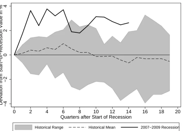
Figure 1 Personal saving rate in 20072009 and previous recessions −4 −2 0 2 4
Deviation from Start−of−Recession Value in %
0 2 4 6 8 10 12 14 16 18 20 Quarters after Start of Recession
Historical Range Historical Mean 2007−2009 Recession
Notes: Saving rate is expressed in percent of disposable income. Deviation from its value at the start of recession in percentage points. Historical Range includes all recessions after 1960Q1. Sources: US Department of Commerce, Bureau of Economic Analysis.
1 Introduction
Fresh interest in personal saving dynamics has been sparked by the remarkable increase in U.S. saving during the Great Recession: For the three years after the business cycle peak in 2007, the personal saving rate remained substantially above its pre-crisis value, and the increase relative to its 2007 value generally exceeded the maximum increase after any previous postwar business cycle peak (see Figure 1). It has long been known that the personal saving rate tends to rise in recessions (seeCarroll(1992) for evidence, and an argument that the pattern reects precautionary motives). This precautionary explanation of cyclical saving dynamics augments an older approach (dating back to some of the
earliest macroeconometric models) which asserted that wealth eects explain the main movements in saving.1,2
A largely separate literature has addressed another longstanding saving puzzle: The steady decline in the U.S. personal saving rate, from over 10 percent of disposable income in the early 1980s to a mere 1 percent in the mid-2000s;3 here, a prominent theme has been the role of nancial liberalization in making it easier for households to borrow. (SeeParker (2000a) for a comprehensive analysis). Some very recent work (Guerrieri and Lorenzoni (2011),Eggertsson and Krugman (2011), Hall (2011)) has argued (without much attempt at empirical precision) that a sudden sharp reversal of this credit-loosening trend played a large role in the recent saving rise.
This paper aims to quantify these three channels, both over the longer span of historical experience and for the period since the beginning of the Great Recession.
To x ideas, the paper begins by presenting (in section 2) a stylized `buer stock' saving model with explicit and transparent roles for each of the inuences emphasized above (the precautionary, wealth, and credit channels). The model's key intuition is that, in the presence of income uncertainty, optimizing households have a target wealth ratio that depends on the usual theoretical considerations (risk aversion, time preference, expected income growth, etc), as well as on two features that have been harder to t into simple stylized models: The degree of labor income uncertainty and the availability of credit. Our model provides a simple analytical formulation that can be used to determine how much saving should go up in response to an increase in uncertainty, or a negative shock to wealth, or a tightening of liquidity constraints.
After section 3's discussion of data and measurement issues, section 4presents a simple nonstructural empirical model, motivated by the theory, that attempts to measure the relative importance of each of these eects (precautionary, wealth, and credit) on the U.S. personal saving rate. A simple OLS regression of the personal saving rate on proxies for the model's three variables (credit, uncertainty, wealth) nds a statistically signicant and economically important role for all three.
Section 5 of the paper constructs a more explicit relationship between the theoretical model and the empirical results, by making a direct identication between the model's parameters (like the measure of unemployment risk) and the corresponding empirical objects (like households' unemployment expectations from the University of Michigan's survey of consumers).
The nal section returns to analysis of the theoretical model, to highlight a particularly interesting implication: In response to a permanent change in economic circumstances (such as a permanent increase in unemployment risk), consumption initially `overshoots' its ultimate permanent adjustment. This reects the fact that, when the target level of wealth
1SeeDavis and Palumbo(2001) for an exposition, estimation, and review.
2The substantial decline in consumption expenditure during and after the 199091 recession was not well explained by the relatively modest changes in household wealth; instead, sluggish spending seemed to be related to a striking degree of pessimism (ex-post justied) about job market conditions during the rst so-called `jobless recovery.'
3Although NIPA accounting conventions impart an ination-related bias to the measurement of personal saving, the downward trend in saving remains obvious even in an ination-adjusted measure of the saving rate.
rises, not only is a higher level of steady-state saving needed to maintain a higher target level of wealth, an immediate further boost to saving is necessary to move from the current (inadequate) level of wealth up to the new (higher) target. An interesting implication is that if the economy suers from costs of adjustment (as most macroeconomic models suggest), even in response to a shock that permanently increases the target saving rate, it might be optimal for a government to engage in transfers designed, at a minimum, to partly counteract the component of the consumption response that reects `overshooting.' In an economy rendered non-Ricardian by the presence of liquidity constraints and/or uncertainty, this provides a potential rationale for countercyclical scal policy targeted at households.
2 Theory: Target Wealth and Credit Conditions
Carroll and Toche(2009) (henceforth CT) provide a tractable framework for analyzing the impact of nonnancial uncertainty, in the specic form of unemployment risk, on household saving. The consumer maximizes the discounted sum of utility from an intertemporally separable CRRA utility function u(•) = •1−ρ/(1 − ρ) subject to the dynamic budget constraint:
mt+1 = (mt−ct)R+`t+1Wt+1ξt+1,
where the next period's market resources mt+1 are the sum of current market resources
net of consumption ct, augmented by the constant interest factor R = 1 +r, and with
the addition of labor income. The level of labor income is determined by the individual's productivity ` (lower case letters designate individual-level variables), the (upper-case)
aggregate wageWt+1 (per unit of productivity) and a zeroone indicator of the consumer's
employment status ξ.
The key feature that makes the model tractable is the assumption that unemployment risk takes a particularly simple form: Employed consumers face a constant probability0of
becoming unemployed; and, once unemployed, the consumer can never become employed again.4 Under these assumptions, CT show that the steady-state target wealth mˇ depends on unemployment risk 0, the interest rate r, the growth rate of wages ∆W, relative risk
aversion ρ, and the discount factor β:5
ˇ m=f(0 (+) , r (+),∆(−)W, ρ(+) , β (+) ). (1)
4We assume here that the employed consumer represents the whole economy. The fact that unemployment rate in the CarrollToche economy converges to 1 can easily be addressed by introducing simple demographics (which do not aect the optimization problem of the employed): Each period new employed consumers are born and a fraction of existing households dies, as inCarroll and Jeanne(2009).
5Specically, the steady-state target wealth can be approximated as ˇ m= 1 + 1 pr( ˆpγ/0)−pγ , wherepr= log (Rβ)1/ρ R,pγ= log (Rβ)1/ρ Γ,pˆγ=pγ(1 +pγω/0),Γ = (1 + ∆W)/(1−0)andω= (ρ−1)/2.
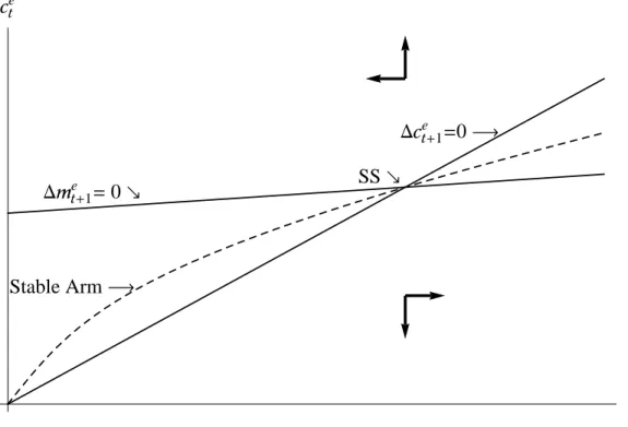
Dcte+1=0 Dmte+1=0 Stable Arm SS mte cte
Figure 2 Consumption Function (Stable Arm of Phase Diagram)
Target wealth increases with unemployment risk, because in response to higher uncertainty, consumers choose to build up a larger precautionary buer of wealth to protect their spending.6 A higher interest rate increases the rewards to holding wealth and thus increases the amount held. Faster income growth translates into a lower wealth target because households who anticipate higher future income consume more now in anticipation of their future prosperity (the `human wealth eect'). Finally, risk aversion and the discount factor have eects on target wealth that are qualitatively similar to the eects of uncertainty and the interest rate, respectively. While the unemployment risk inCarroll and Toche(2009) is of a simple form, the key mechanisms at work are the same as those in more sophisticated setups with a realistic specication of uninsurable risks (building on the work of Skinner (1988),Zeldes (1989),Deaton (1991),Carroll (1997) and others).
Figure 2 shows the phase diagram for the CT model. The consumption function is indicated by the dashed line, which is the saddle path that leads to the steady state at which the ratios of both consumption and market resources to income (c and m) are
constant.
Explicit liquidity constraints were deliberately omitted from the CT model to emphasize the conceptual point that uncertainty induces concavity of the consumption function (that is, a higher marginal propensity to consume for people with low levels of wealth) even in
6Note that the increase in0is a pure increase in risk because productivity is assumed to grow by the factor1/(1−0) each period,`t+1=`t/(1−0)(seeCarroll and Toche(2009), p. 6).
the absence of constraints (for a general proof of this proposition, seeCarroll and Kimball (1996)). Indeed, because the employed consumer is always at risk of a transition into the unemployed state where income will be zero, the `natural borrowing constraint' in this model prevents the consumer from ever choosing to go into debt, because an indebted unemployed consumer with zero income might be forced to consume a negative amount to satisfy the budget constraint.
We make only one modication to the CT model for the purpose at hand: We in-troduce an `unemployment insurance' system that guarantees a positive level of income for unemployed households. Now, households with low levels of market resources will be willing to borrow because they will not starve even if they become unemployed. The eect of this change is simply to induce a leftward shift in the consumption function by an amount corresponding to the present discounted value of the unemployment benet. The consumer will limit his indebtedness, however, to an amount small enough to guarantee that consumption will remain strictly positive even when the consumer is unemployed (this is the `natural borrowing constraint' in this model).
We could easily add a tighter `articial' borrowing constraint, imposed exogenously by the nancial system, which prevents the consumer from borrowing all the way up to the natural borrowing constraint. But Carroll(2001a) shows that the eects of tightening an articial constraint are qualitatively and quantitatively similar to the eects of tighten-ing the `natural' borrowtighten-ing constraint; while we do not doubt that `articial' borrowtighten-ing constraints (that is, ones tighter than those imposed by the budget constraint and the utility function) are important, we do not incorporate them into our framework since we can capture their consequences by manipulating the natural borrowing constraint that is already an intrinsic element of the model. As our empirical estimates will suggest below, the process of nancial liberalization which began in the U.S. in the early 1980s and arguably continued until the eve of the Great Recession could be interpreted as a process of continual easing of credit constraints which put a downward pressure on the saving rate.
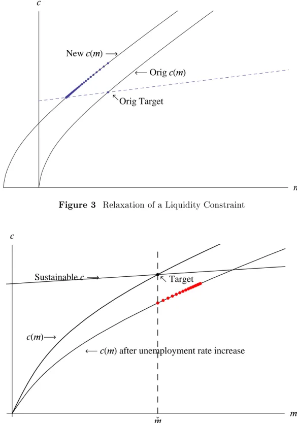
Figure3shows that the model reproduces the standard result from the existing literature (see, e.g.,Carroll(2001b),Muellbauer(2007),Guerrieri and Lorenzoni(2011),Hall(2011)): Relaxation of the borrowing constraint leads to an immediate increase in consumption for a given level of resources. But the higher spending causes the consumer's level of wealth to decline, forcing a corresponding decline in consumption until wealth eventually settles at its new, lower target level.
The eects of an increase in unemployment risk are depicted in the next gure. Quali-tatively, the eects are essentially the opposite of a credit loosening: When unemployment risk goes up, the level of consumption falls sharply as consumers begin the process of accumulation toward a higher target wealth ratio.7
7The model is specied in such a way that an increase in the parameter0that we are calling the `unemployment risk' here actually induces an osetting increase in the expected mean level of income (an increase in0 is a mean-preserving
spread in the relevant sense); the spending of a consumer with certainty-equivalent preferences therefore would not change in response to a change in0, so we can attribute all of the increase in the saving rate depicted in the gure to the precautionary motive.
!Orig Target !Orig!!"" New!!"""
" !
Figure 3 Relaxation of a Liquidity Constraint
Sustainablec
cHmLafter unemployment rate increase Target
cHmL
mÇ m
c
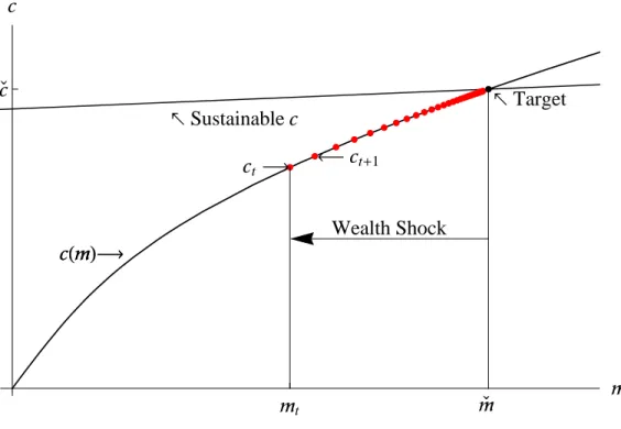
Sustainablec cHmL ct ct+1 Wealth Shock Target cHmL mÇ mt m cÇ c
Figure 5 A Wealth Shock
In sum, the model emphasizes three factors that aect saving and that might vary substantially over time. First, because the precautionary motive diminishes as wealth rises, the saving rate is a declining function of market resourcesmt. Second, since an expansion
in the availability of credit reduces the target level of wealth, looser credit conditions CEAt lead to lower saving. Finally, higher unemployment risk 0t results in greater saving for precautionary reasons.
Qualitatively, the framework thus implies that a reduced-form regression for the saving rate st
st =γ0+γmmt+γCEACEAt+γ00t+γ0Xt+εst (2) gives the following estimates:
γm <0, γCEA <0, γ0 >0, γ0 ≈0, (3) where CEAt denotes the Credit Easing Accumulated index, a measure of credit supply (described in detail below), and the vector Xt collects other drivers of saving that are outside the scope of the model, such as demographics, corporate and government saving, etc. After discussing our data we estimate regressions of the form (2) in section4 below.
3 Data and Measurement Issues
We use U.S. quarterly data for 1966Q22011Q1.8 The saving rate is from the BEA's National Income and Product Accounts and is as a percentage of disposable income.9,10
Market resources mt are measured as the ratio of household net worth to disposable income, in line withCarroll and Toche(2009).11,12 Our measure of credit supply conditions, which we call the Credit Easing Accumulated index (CEA, see Figure 6) is constructed in the spirit of Muellbauer (2007) and Duca, Muellbauer, and Murphy (2010) using the question on consumer installment loans from the Federal Reserve's Senior Loan Ocer Opinion Survey (SLOOS) on Bank Lending Practices (see also Fernandez-Corugedo and Muellbauer (2006) and Hall (2011)). The question asks about banks' willingness to make consumer installment loans now as opposed to three months ago. To calculate a proxy for the level of credit conditions, the scores from the survey were accumulated, weighting the responses by the debtincome ratio to account for the increasing trend in that vari-able.13 (The index is normalized between 0 and 1 to make the interpretation of regression coecients straightforward.)
The Credit Easing Accumulated Index (CEA) measures the availability/supply of credit to a typical household through factors other than the level of interest ratesfor example, through loan to value and loan to income ratios, availability of mortgage equity with-drawal and mortgage renancing. The broad trends in the CEA index correlate strongly with measures nancial reforms of Abiad, Detragiache, and Tressel (2008), measures of banking deregulation of Demyanyk, Ostergaard, and rensen (2007) (see panel A of their Figure 1, p. 2786).14 In addition, they seem to reect well the key developments of the
8Most time series were downloaded from Haver Analytics, and were originally compiled by the Bureau of Economic Analysis, the Bureau of Labor Statistics or the Federal Reserve. The beginning of the estimation sample was determined by the availability of our empirical measure of credit conditions.
9As a robustness check, we have also re-estimated our models with alternative measures of saving: Gross household saving as a fraction of disposable income, gross and net private saving as a fraction of GDP, ination-adjusted personal saving rate and two measures of saving from the Flow of Funds (which include/exclude durables). The ination-adjusted saving rate deducts from saving the erosion of money-denominated assets due to ination. The the Flow of Funds (FoF) calculates saving as the sum of the net acquisition of nancial assets and tangible assets minus the net increase in liabilities. Because this FoF-based measure is substantially more volatile, the t of the model is worse than for the NIPA-based PSR. However, the main messages of the paper remain unchanged.
10Many reasonable objections can be made to this, or any other, specic measure of the personal saving rate, including the treatment of durable goods, the treatment of capital gains and losses, and so on. While some defense of the NIPA measure could be made in response to many of these challenges, such defenses would take us too far aeld, and we refer the reader to the extensive discussions of these measurement issues that date at least back toFriedman(1957).
11The literature on precautionary saving typically measures wealth as a ratio to permanent income. Permanenttransitory decomposition in which income consists of unobserved random walk and white noise assigns almost all variation in (measured) income to its permanent component, so that both indicators practically coincide. This is not surprising because, as is well-known (and also documented in Appendix 2), it is dicult to reject the proposition that almost all shocks to the level of aggregate income are permanent; autocorrelation functions and partial autocorrelation functions indicate that log-level of disposable income is close to a random walk; see our further discussion in Appendix 2.
12This variable is lagged by one quarter to account for the fact that data on net worth are reported as the end-of-period values.
13As inMuellbauer(2007), we use the question on consumer installment loans rather than mortgages because the latter is only available starting in 1990Q2 and the question changed in 2007Q2. Our CEA index diers fromMuellbauer(2007)'s Credit Conditions Index in that Muellbauer accumulates raw answers, not weighting them by the debtincome ratio.
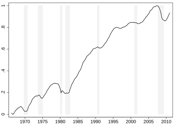
Figure 6 The Credit Easing Accumulated (CEA) Index 0 .2 .4 .6 .8 1 1970 1975 1980 1985 1990 1995 2000 2005 2010
Notes: ShadingNBER recessions.
Sources: Federal Reserve, accumulated scores from the question on change in the banks' willingness to provide consumer installment loans from the Senior Loan Ocer Opinion Survey on Bank Lending Practices,http://www.federalreserve.gov/boarddocs/snloansurvey/.
U.S. nancial market institutions as described in McCarthy and Peach (2002), Dynan, Elmendorf, and Sichel (2006), Green and Wachter (2007), and Campbell and Hercowitz (2009), among others. Until the early 1980s, the U.S. consumer lending markets were quite heavily regulated and segmented. After the phaseout of interest rate controls, the markets became more competitive, spurring nancial innovations that led to greater access to credit. Technological progress leading to new nancial instruments and better credit screening methods, a greater role of nonbanking nancial institutions, and the increased use of securitization all contributed to the dramatic rise in credit availability from the early 1980s until the onset of the Great Recession in 2007. The subsequent signicant drop in the CEA index was associated with the funding diculties and de-leveraging of nancial institutions. As a caveat, it is important to realize that CEA is presumably inuenced to some degree by business-cycle conditions over the short term. However, we have veried that our results do not materially change when we use the credit conditions index ofDuca, Muellbauer, and Murphy (2010), which diers from our CEA in that Duca, Muellbauer, and Murphy explicitly remove identiable eects of interest rates and the macroeconomic outlook from the SLOOS data using regression techniques.15 Since the results are similar using both measures, our interpretation is that our measure captures secular more than cyclical movements in credit.
We measure a proxy Etut+4 for unemployment risk 0t using a re-scaled answers to the question about expected change in unemployment in the University of Michigan Survey of Consumer Sentiment.16 In particular, we estimate
Etut+4 using tted values∆4uˆt+4 from
the regression of the four-quarter-ahead change in unemployment rate ∆4ut+4 ≡ut+4−ut on the answer in the survey, summarized with a balance statistic UExpBS
t :
∆4ut+4 = α0+α1UExpBSt +εt+4,
Etut+4 = ut+ ∆4uˆt+4.
The series, whichas expectedcorrelates strongly with unemployment rate and precedes its dynamics, is shown in Figure7.
4 Reduced-Form Saving Regressions
Before proceeding to structural estimation of the model of section2we investigate a simple reduced-form benchmark:
st=γ1+γmmt+γCEACEAt+γEuEtut+4+γtt+γ0Xt+εst. (4) Such a specication can be readily estimated using the OLS and IV estimators, and at a minimum can be interpreted as summarizing basic stylized facts about the data.
(in data from the American Housing Survey, 19792007), an indicator which is arguably to some extent aected by uctuations in demand.
15We would like to thank John Duca and John Muellbauer for sharing their CCI data.
16The relevant question is: How about people out of work during the coming 12 monthsdo you think that there will be more unemployment than now, about the same, or less?
Figure 7 Unemployment Risk Etut+4 and Unemployment Rate (Percent) 2 4 6 8 10 1970 1975 1980 1985 1990 1995 2000 2005 2010
Legend: Unemployment rate: Thin black line, Unemployment risk Etut+4: Thick red/grey line.
ShadingNBER recessions.
Sources: University of Michigan Survey of Consumer Sentiment,
Figure 8 The Fit of the Baseline Model and the Time TrendActual and Fitted PSR (Percent of Disposable Income) (Percent of Disposable Income)
2 4 6 8 10 12 1970 1975 1980 1985 1990 1995 2000 2005 2010
Legend: Actual PSR: Thin black line, Baseline model: Thick red/grey line, Time trend: dashed black line. ShadingNBER recessions.
Table 1 reports the estimated coecients from several variations on equation (4). The rst four columns show univariate specications in which the saving rate is in turn regressed on each of the three determinants analyzed above: Wealth, credit conditions and unem-ployment risk. In each specication we include the time trend to investigate how much each regressor contributes to explaining the PSR beyond the portion captured mechanically by the linear time eects. The three coecients have the signs predicted by the model of section 2and are statistically signicant. Univariate regressions capture up to 85 percent of variation in saving.17
But the univariate models on their own do not adequately describe the dynamics of the PSR. As the model (All 3) in the fth column shows, the three key variables of interest wealth and credit conditionsjointly explain roughly 90 percent of the variation in the saving rate over the past ve decades. As expected, the point estimates again indicate a strong negative correlation between saving and net wealth and credit conditions and a positive correlation with unemployment risk. Interestingly, once the three variables are included jointly, the time trend ceases to be signicant, which is in line with the fact that the three models in columns 24 have higher R¯2 that the univariate model with the time
trend only.18
The specication in column 5 (All 3) suggests that a more parsimonious version of the model without the time trend reported in column 6 (Baseline)and also suggested by the structure of section 2neatly summarizes the key features of the saving rate. The estimated coecient on net wealth implies the (direct) long-run marginal propensity to consume of about 1.2 cents out of a dollar of (total) wealth. The value is relatively low compared to much of the literature, which typically estimates the marginal propensity to consume out of wealth (MPCW) of about 37 cents without explicitly accounting for credit conditions.19 However, in a univariate model regressing the PSR just on net wealth (not reported here), the implied MPCW is about 4.3 percent, in line with the literature. (This suggests that much of what has been interpreted as pure wealth eects in the prior literature may actually have been attributable to precautionary or credit availability eects that are correlated with wealth).
The coecient on the Credit Easing Accumulated Index is highly statistically signicant with atstatistic of−10.7. The point estimate ofγCEAimplies that increased access to credit
during the sample period ending in 2007 (before the Great Recession) reduced the PSR by about 6 percentage points of disposable income. In the aftermath of the Recession, the CEA index declined between 2007 and 2010 by roughly0.11as the credit supply tightened,
17Because the rst four models only include 12 explanatory variables, adjustedR2and plainR2practically coincide.
18Estimating univariate saving regressions without the time trend, results in higher R¯2 for wealth and the credit
conditions0.72 and 0.80, respectivelythat for the time model in column one (0.70). (Because unemployment risk is not trending, it captures relatively little variation in saving on its own (about 10 percent) but is important in addition to the two other factors, as illustrated in columns 4 and 5.)
19See, for example, Skinner(1996), Ludvigson and Steindel (1999), Lettau and Ludvigson (2004), Case, Quigley, and
Shiller(2005), andCarroll, Otsuka, and Slacalek(2011). SeeMuellbauer(2007) andDuca, Muellbauer, and Murphy(2010) for a model which includes a measure of credit conditions in the consumption function.
contributing to roughly a0.64percentage point increase in the PSR (see the discussion of
Table 3 below for more detail).
Figure 8 further illustrates why we nd the baseline specication in column 6 more appealing than the more atheoretical model with a linear time trend. The trends in saving and the CEA are both non-linear, moving consistently with each other even within our sample and often persistently departing from the linear trend (as documented also by its substantially lower R¯2). In addition, it is likely that the time-only model will
become increasingly problematic as observations beyond our sample accumulate, arguably providing additional evidence on the structural break in the time model during the Great Recession.20
Finally, the last model investigates the joint eect of credit conditions and unemployment risk. The structural model of section 2 implies that uncertainty aects saving more strongly when credit constraints bind tightly; the model in column 7 (Interact) conrms the prediction with a (borderline) signicant negative interaction term between the CEA and unemployment risk.21
Table 2 presents a second battery of specication checks of the baseline model (shown again for reference in the rst column). The second model (Uncertainty) investigates the eects of adding to the baseline regression an alternative proxy for uncertainty: theBloom, Floetotto, and Jaimovich (2009) index of macroeconomic and nancial uncertainty.22 The new variable is statistically insignicant and the coecients on the previously included variables are broadly unchanged, suggesting that our baseline uncertainty measure is more appropriate for our purposes (which makes sense, as personal saving is conducted by persons, whose uncertainty is likely better captured by our measure of labor income uncertainty than by the Bloom, Floetotto, and Jaimovich (2009) measure of rm-level shocks).
The third model (Lagged st−1) explores the implications of adding lagged saving to
the list of regressors. The coecient is highly statistically signicant, consistent with the `stickiness' in consumption growth implied by the model of section 2 (for more extensive international evidence see also Carroll, Slacalek, and Sommer (forthcoming)). However, this positive autocorrelation only captures near-term stickiness and has little eect on the long-run dynamics of saving. Indeed, the coecients from the baseline roughly equal their long-term counterparts from the model with lagged saving rates (that is, coecient estimates pre-multiplied by 2.5, or 1/(1−γs) = 1/(1−0.60)).23
The fourth model (Debt) explores the role of the debtincome ratio. The variable could be relevant for two reasons. First, it could partly account for the fact that debt is held by a dierent group of people than assets and consequently net worth might be an
20Reliable PSR data only start in 1959 and document that the downward trend in saving started around 1975, so that our sample is actually quite favorable to the time-only model.
21Adding an interaction term between the CEA and wealth results in a borderline signicant positive estimate, which is in line with the concavity of the consumption function, show in Figure2.
22SeeBaker, Bloom, and Davis(2011) for related work measuring economic policy uncertainty.
23Note that with the inclusion of lagged saving, the DurbinWatson statistic becomes close to 2, suggesting that whatever serial correlation problems exist in the other specications reect simple rst order autocorrelation of the errors.
Figure 9 The Fit of the Baseline Model and the Model with Full Controls (of Table 2)Actual and Fitted PSR (Percent of Disposable Income)
2 4 6 8 10 12 1970 1975 1980 1985 1990 1995 2000 2005 2010
Legend: Actual PSR: Thin black line, Baseline model: Thick red/grey line, Model with full control variables: dashed black line. ShadingNBER recessions.
Sources: Bureau of Economic Analysis, authors' calculations.
insucient measure of wealth. Second, debt might also reect credit conditions (although as mentioned abovewe prefer the CEA index because it in our view better isolates the role of credit supply from demand). The regression can thus also be interpreted as a horse-race between the CEA and the debtincome ratio. In any case, while the coecient γd has the correct (negative) sign, it is statistically insignicant and its inclusion does not substantially aect estimates obtained under the baseline specication.
The fth model (Full Controls) controls for the eects of other potential determinants of household saving: expected real interest rates, expected income growth, and government and corporate saving (both measured as a percent of GDP).24 Some of these factors are statistically signicant, but are inconsequential in economic terms. Figure 9 makes it clear that while these additional factors were potentially important during specic episodes (especially in the early 1980s), they have on average had only a limited impact
24Expected real interest rates and expected income growth are constructed using data from the Survey of Professional Forecasters of the Philadelphia Fed.
on U.S. household saving. The negative coecient on corporate saving is consistent with the proposition that households may `pierce the corporate veil' to some limited extent25 but there is no evidence for any interaction between personal and government saving. One interpretation of this is that `Ricardian' eects that some prior researchers have claimed to nd might instead reect reverse causality: Recessions cause government saving to decline at the same time that personal saving increases (high unemployment, falling wealth, restricted credit) but for reasons independent of the Ricardian logic (reduced tax revenues and increased spending on automatic stabilizers, e.g.). Since we are controlling directly for the variables (wealth, unemployment risk, credit availability) that were (in this interpretation) proxied by government saving, we no longer nd any eect of government saving on personal saving.
When the model is estimated only using the post-1980 data in the sixth column (Post-1980), its t measured by theR¯2 actually improves, in contrast with some other economic
relationships, whose goodness-of-t deteriorated in the past 20 years. The F test is consistent with the proposition that the coecients of the regression have not changed over the sample.
Finally, to explore how much endogeneity may matter,26 the specication IV re-estimates the baseline specication using the IV estimator. Instruments are the lags of net wealth, unemployment risk andcruciallythe Financial Liberalization Index of Abiad, Detra-giache, and Tressel (2008) (described in Appendix 1). The FLI is an alternative measure of credit conditions constructed using the records about legal and regulatory changes in the banking sector. The index intends to capture exogenous changes in credit conditions. While it is a rough approximation as it reects only the most important events (see also Figure 14 in Appendix 1), the prole of the FLI matches well that of the CEA. The estimated coecients remain broadly unchanged compared with the baseline specication. Interestingly, the test of overidentifying restrictions does not reject the hypothesis that factors such as unemployment or uncertainty do not exert much inuence on the saving rate beyond their (potential) impact on net wealth and credit conditions.
We have also estimated specications with other variables, whose detailed results we do not report. As inParker(2000b), demographic variables, like the old-age dependency ratio, were insignicant in our regressions. The importance of population aging in crosscountry studies of household saving (for example, Bloom, Canning, Manseld, and Moore (2007) andBosworth and Chodorow-Reich(2007)) appears to be largely driven by the experience of Japan and Koreacountries well ahead of the United States in the population aging process.
To address a potential criticism that saving rate regressions are dicult to interpret because aggregate income shocks reect a mix of transitory and persistent factors, we
25Regressions with total private saving as a dependent variable yield qualitatively similar results as our baseline estimates in Table1.
26As mentioned above, wealth is lagged by one quarter to alleviate endogeneity in OLS regressions. However, a standard concern about reduced-form regressions like (4) is that the OLS coecient estimates might be biased because the regressions do not adequately account for all relevant right-hand size variables (such as expectations about income growth; see also Appendix 2 for further discussion).
have also re-estimated our regressions with alternative measures of disposable income (see Appendix 2) which exclude a range of identiable temporary shocks such as scal stimulus and extreme weather. There was little econometric evidence that transitory movements in aggregate disposable income are substantial and our econometric results basically did not change.27
Table3reports in-sample t of the baseline model and the model Interact with the CEA uncertainty interaction term of Table1, and the contributions of the individual variables to the explained increase in the saving rate between 2007 and 2010. Two principal conclusions emerge. First, both models (especially the latter) are able to capture well the observed change in the saving rate. Second, the key explanatory factors in saving over the past two years were the changes in wealth and uncertainty, with credit conditions (as measured by CEA) playing a less important role. While the change in the trajectory of the CEA index is quite striking (see Figure 6), and may explain the sudden academic interest in the role of household credit over the business cycle (see the papers cited in the introduction), this evidence suggests that the rise in saving cannot be mainly attributed to the decline in credit availability. If correct, this nding is particularly important at the present juncture because it suggests that however much the health of the nancial sector continues improving, the saving rate is likely to remain high so long as uncertainty remains high and household wealth remains impaired (compared, at least, to its previous heights).
5 Structural Estimation
Preliminary
This section estimates the structural model of section 2 by minimizing the distance between the data on saving implied by the model and those observed in reality. The nonlinear least squares (NLLS) procedure we use has some advantages over the reduced-form regressions. Besides arguably being more immune to endogeneity and suitable for estimating structural parameters (such as the discount factor), it imposes on the data a structure that makes them easier to interpret. In particular, the model identies the target wealth, which varies depending on the evolution of risk and credit conditions, and which can in principle be useful for identifying major deviations of actual wealth from the optimal level desired by consumers and gauging future trends in the saving rate. As Figure 2 documents, the structural model explicitly justies and disciplines non-linearities, which can be important especially during turbulent times, when the shocks are large enough to move the system far from its steady state. In such times, estimation of linear or linearized models may be subject to substantial error.
27Interestingly, an auxiliary regression of income growth on the lagged saving rate in the spirit ofCampbell(1987) yields a statistically-insignicant slope when post-1985 data are included (see Appendix 2).
5.1 Estimation Procedure
We assume households instantaneously observe exogenous movements in the three factors: wealth shocksm, unemployment risk 0 and credit supply conditions CEA, and that they
consider the shocks to 0 and CEA to be permanent (and do not expect the shocks to
wealth to be reversed).28 Given these factors and the parameters, each period consumers re-optimize their consumptionsaving choice (described in section 2). Collecting the pa-rameters in the vectorΘand denoting the target wealthmˇt(·)and the corresponding wealth gapmt−mˇt, the model implies a series of saving ratessttheor(Θ;mt−mˇt), which we match to those observed in the data, smeast . Our estimates Θˆ thus solve the following problem:
ˆ Θ = arg min T X t=1
stmeas−stheort Θ;mt−mˇ m¯(CEAt),0(Etut+4)
2
, (5)
where the target wealth mˇ depends on the credit conditions and unemployment risk as
described in section2. In our baseline specication the parameter vector Θconsists of the
discount factor β and the scaling constants for credit conditions and unemployment risk:
Θ = {β,θ¯m, θCEA,θ¯0, θu}, (6)
¯
mt = θ¯m+θCEACEAt, (7)
0t = θ¯0+θuEtut+4. (8)
The re-scaling ensures that the unitless measure of credit conditions is re-normalized as a fraction of disposable income and that the expected unemployment rate is transformed into the model-compatible equivalent of permanent risk. The model implies thatθCEA >0
and θu >0.
Minimization (5) is a non-linear least squares problem in which the standard asymptotic results apply. Standard errors for the estimated parameters are calculated using the delta method as follows.29 Dene the scores q
t(Θ) = smeast −stheort (Θ) ∂stheort (Θ) ∂Θ0 and the 5×5 matrices E = var qt(Θ) and D = E∂qt(Θ)
∂Θ0 . The estimates have the asymptotic distribution:
T1/2( ˆΘ−Θ) →dN(0, D−1ED0−1).
Because the saving function stheort (Θ) is not available in the closed form, we calculate its
partial derivatives numerically.
28The assumption that households believe the shocks to be permanent is necessary for us to be able to use the tractable model we described earlier in the paper. While indefensible as a literal proposition (presumably nobody believes the unemployment rate will remain high forever), the high serial correlation of these variables means that the assumption may not be too objectionable. In any case, a model that incorporated more realistic descriptions of these processes would be much less transparent and might not be computationally feasible with present technology.
29To construct the objective function (which we then minimize overΘ) we need to solve the consumer's optimization for each quarter. Because the calculation is computationally demanding, we cannot apply bootstrap to calculate standard errors. (The ShapiroWilk test does not reject normality of residuals.)
5.2 Results
Table 4 summarizes the calibration and the estimation results. The calibrated
parametersreal interest rate r = 0.04/4, wage growth ∆W = 0.01/4 and the coecient
of relative risk aversion ρ = 2 take their standard (quarterly) values and meet (together
with the discount factor β) the conditions sucient for the problem to be well-dened.
The discount factor β = 1−0.0064 = 0.9936, or 0.975 at annual frequency, lies in the
standard range.
Figure 10 shows the estimated horizontal shift in the consumption function m¯t. The
estimates of the scaling factors θ¯m and θCEA imply that m¯t varies roughly between 0 and
(−0.0071 + 5.2208)/4 = 1.3, implying that nancial deregulation resulted at its peak in
providing credit of roughly 130% of annual income.
Figure 11shows the estimated quarterly intensity of permanent unemployment risk. Figure 12 shows the t of the structural model. In terms of R¯2 (Table 4), the model
captures more than 80 percent of variation in the saving rate, doing only slightly worse than our baseline reduced-form model (whose R¯2 is roughly 0.9). The MincerZarnowitz horse
race between the models puts roughly 0.45 on the structural model (although the high standard error on the coecient suggests high correlation between the two model-implied saving rates).
Figure 13 decomposes the explained PSR by the three explanatory factors as follows. Given the estimated parametersΘ(from Table4) we switch o the uncertainty and credit
supply channels by setting the values of these series equal to their means. This means that, e.g., the dierence between the model tted series (red/grey line and the tted series excluding uncertainty (black line) in Figure 12 is to be interpreted as the eects of time variation in unemployment risk0 rather than total extent of the precautionary motive.
While the wealth uctuations do contribute to a good performance of the model at the business-cycle frequencies, the CEA is essential in capturing the trend decline in the PSR between the 1980s and the early 2000s. The counter-cyclical uctuations in the uncertainty contribute the the increases in the PSR during recessions, including the last one.
6 Conclusions
We nd evidence that credit availability, household wealth, and movements in income uncertainty have all been important factors in driving U.S. household saving over the past 40 years. In particular, a relentless expansion of credit supply between the mid-1980s and 2007 (likely largely reecting nancial innovation and liberalization) and the higher asset values and net wealth (possibly also partly attributable to the credit boom) encouraged households to save less out of their disposable income. At the same time, the uctuations in net wealth and labor income uncertainty, for instance during and after the burst of the information technology and credit bubbles of 2001 and 2007, can explain the bulk of business cycle uctuations in personal saving.
Figure 10 Estimated Extent of Credit Constraints m¯t (Fraction of Quarterly Disposable Income) 1970 1975 1980 1985 1990 1995 2000 2005 2010 0 0.5 1 1.5 2 2.5 3 3.5 4 4.5 5 5.5
Notes: ShadingNBER recessions.
Sources: Federal Reserve, accumulated scores from the question on change in the banks' willingness to provide consumer installment loans from the Senior Loan Ocer Opinion Survey on Bank Lending Practices, http://www.federalreserve.gov/boarddocs/snloansurvey/, authors' calculations.
Figure 11 Estimated Permanent Unemployment Risk 0t 1970 1975 1980 1985 1990 1995 2000 2005 2010 5.5 6 6.5 7 7.5 8 8.5 9x 10 −5
Notes: ShadingNBER recessions.
Sources: University of Michigan Survey of Consumer Sentiment,
Figure 12 Fit of the Structural ModelActual and Fitted PSR (Percent of Disposable Income) 1970 1975 1980 1985 1990 1995 2000 2005 2010 0 2 4 6 8 10 12
Legend: Actual PSR: Thin black line, Structural model: Thick red/grey line. ShadingNBER recessions.
Figure 13 Decomposition of Fitted PSR (Percent of Disposable Income) 1970 1975 1980 1985 1990 1995 2000 2005 2010 0 2 4 6 8 10 12 Fitted PSR
Fitted PSR excl. Uncertainty
Fitted PSR excl. Uncertainty and CEA
Notes: ShadingNBER recessions.
Other determinants of saving suggested by various literatures (e.g., scal decits, demo-graphics, income expectations) either work through the key factors above, are of second-order importance, or matter only during particular episodes. These ndings are broadly in line with the complementary household-level evidence reported in Dynan and Kohn (2007), Moore and Palumbo (2010), Bricker, Bucks, Kennickell, Mach, and Moore (2011) and Petev, Pistaferri, and Eksten (2011).30 Of course, all this evidence is based on historical data and, going forward, factors such as rapidly rising federal debt or retirement of baby-boomers could yet lead to new structural shifts in household saving. From a more conjunctural perspective, our results suggest that the PSR will remain substantially higher than before the crisis for some time given strict lending standards and below-target wealth.
30Dynan and Kohn(2007) nd that data from the Federal Reserve's Survey of Consumer Finances (SCF) and the Michigan Survey of Consumer Sentiment show too little variation in the measures of impatience, risk aversion, expected income, interest rates and demographics to adequately explain the household indebtedness. In contrast, they argue that house prices and nancial innovation have been important drivers of indebtedness. Moore and Palumbo(2010) document that the drop in consumer spending during the Great Recession was accompanied by signicant erosions of home and corporate equity held by households. Using SCF data,Bricker, Bucks, Kennickell, Mach, and Moore(2011) document higher desired precautionary saving among most families during the Great Recession. Petev, Pistaferri, and Eksten(2011) discuss the following factors behind the observed changes in consumption during the Great Recession: the wealth eect, an increase in uncertainty and the credit crunch.
Appendix 1: Comparison of Alternative Measures of
Credit Availability
Figure 14 compares three measures of credit availability: our baseline CEA index, the Index of Financial Liberalization constructed of Abiad, Detragiache, and Tressel (2008) and the ratio of household liabilities to disposable income.
The Abiad, Detragiache, and Tresselindex is a mixture of indicators of nancial development: credit controls and reserve requirements, aggregate credit ceilings, interest rate liberalization, banking sector entry, capital account transactions, development of securities markets and banking sector supervision.
For comparison, the gure also includes the ratio of liabilities to disposable income (from the Flow of Funds), which is admittedly determined by the interaction between credit supply and demand.
Figure 14 Alternative Measures of Credit Availability .6 .7 .8 .9 1
IMF Index of Financial Liberalization
0 .5 1 1.5 CEA/Debt−Income Ratio 1970 1975 1980 1985 1990 1995 2000 2005 2010
Legend: Debtdisposable income ratio: Thin black line, CEA index: Thick red/grey line, the IMF Index of Financial Liberalization: dashed black line. ShadingNBER recessions.
Sources: Federal Reserve, accumulated scores from the question on change in the banks' willingness to provide consumer installment loans from the Senior Loan Ocer Opinion Survey on Bank Lending Practices, http://www.federalreserve.gov/boarddocs/snloansurvey/; Abiad, Detragiache, and Tressel(2008); Flow of Funds, Board of Governors of the Federal Reserve System.
Figure 15 Growth of Real Disposable Income (Percent) −10 0 10 20 1970 1975 1980 1985 1990 1995 2000 2005 2010
Legend: BEA disposable income: Thick red/grey line, Less cleaned disposable income series: Thin black line, More cleaned disposable income series: dashed black line.
Notes: ShadingNBER recessions.
Sources: Bureau of Economic Analysis, authors' calculations.
Appendix 2: Stochastic Properties of Aggregate
Disposable Income
Measurement of Disposable Income
This appendix investigates the properties of three measures of disposable income: the ocial series produced by the BEA and two cleaned series, in which we try to exclude transitory income shocks due to temporary events, such as weather and scal policy. Specically, we have removed the following events from the ocial disposable income series using regressions:
• The dollar amounts of temporary rebate checks during 1975, 2008, and 2009 scal stimulus episodes.
Figure 16 Personal Saving Rate (Percent of Disposable Income) 2 4 6 8 10 12 1970 1975 1980 1985 1990 1995 2000 2005 2010
Legend: BEA personal saving rate: Thick red/grey line, PSR calculated with the less cleaned income series: Thin black line, PSR calculated with the more cleaned income series: dashed black line.
Notes: ShadingNBER recessions.
Sources: Bureau of Economic Analysis, authors' calculations.
• Dummies for quarters with unusually high or low cooling degree days, and unusually high or low heating degree days (the dummy has a value of 1 whenever the seasonally-adjusted series are more than 2 standard deviations above or below its mean).
• Dummies for quarters with unusually high or low national temperature, and unusually high or low precipitation (again, using the 2 standard deviations criterion).
• Separate dummies for snowstorms or heat waves which were deemed unusually extensive and damaging (these events do not necessarily overlap with the episodes identied from the national temperature and cooling/heating degree days data).
Stochastic Properties of Disposable Income and Saving for a Rainy Day
The classic paper byCampbell (1987) has derived that the permanent income hypothesis implies that saving is negatively related to future expected income growth. This appendix investigates the univariate stochastic properties of disposable income and the relationship between saving and income, or the lack of it, in Tables5 and6, respectively.Table5documents that all three disposable income series are statistically indistinguishable from a random walk. This means that the series are unpredictable using their own lags. In particular, for the income series in log-level, the rst autocorrelations are very close to 1 and the augmented DickeyFuller test does not reject the null of a unit root. In contrast, for income growth, the rst and other autocorrelations are zero, as also documented by the p values of the BoxLjung Q statistic, and the ADF test (of course) strongly rejects a unit root.
Table 6 reports the estimates ofα1 the sensitivity of the saving rate to future income growth:
st=α0+α1∆yt+1+εt, (9)
which is motivated byCampbell(1987), who derives that under the permanent income hypothesis the coecient α1 is negative, as households save more when they are pessimistic about future income growth.
Overall, the estimates suggest that coecient α1 is statistically insignicant and small, es-pecially when the full sample, 1966Q22011Q1, is used and when income growth ∆yt+2 enters the regression (9), which might be justied because of time aggregation issues. While there is some evidence of a negative coecient in the pre-1985 sample (which overlaps with the sample 1953Q21984Q4 considered by Campbell (1987)), the relationship seems to break down in the past 20 years.
Table 1 Preliminary regressions with time trend
st=γ0+γmmt+γCEACEAt+γEuEtut+4+γtt+γuC(Etut+4×CEAt) +εt
Model Time Wealth CEA Un Risk All 3 Baseline Interact
γ0 11.954∗∗∗ 22.596∗∗∗ 9.321∗∗∗ 8.241∗∗∗ 13.772∗∗∗ 14.043∗∗∗ 14.181∗∗∗ (0.608) (1.414) (0.574) (0.420) (2.143) (1.819) (2.112) γm −2.606∗∗∗ −1.124∗∗∗ −1.183∗∗∗ −1.368∗∗∗ (0.319) (0.423) (0.347) (0.456) γCEA −14.138∗∗∗ −5.472∗∗∗ −6.121∗∗∗ −4.604∗∗∗ (1.736) (1.936) (0.573) (1.721) γEu 0.670∗∗∗ 0.316∗∗∗ 0.287∗∗∗ 0.385∗∗∗ (0.055) (0.117) (0.075) (0.108) γt −0.044∗∗∗ −0.025∗∗∗ 0.042∗∗∗ −0.048∗∗∗ −0.005 0.004 (0.005) (0.003) (0.011) (0.002) (0.014) (0.014) γuC −0.321∗∗ (0.158) ¯ R2 0.703 0.846 0.825 0.881 0.895 0.895 0.899 F stat p val 0.00000 0.00000 0.00000 0.00000 0.00000 0.00000 0.00000 DW stat 0.305 0.686 0.500 0.863 0.936 0.933 0.980
Notes: Estimation sample: 1966Q22011Q1.{∗,∗∗,∗∗∗}=Statistical signicance at{10,5,1}percent. NeweyWest standard
Table 2 Personal saving rateConstant target wealth models
st=γ0+γmmt+γCEACEAt+γEuEtut+4+γσσt+γsst−1+γddt+. . .
. . . +γrrt+γGSGSt+γCSCSt+εt
Model Baseline Uncertainty Laggedst−1 Debt Full Controls Post-1980 IV
γ0 14.043∗∗∗ 13.869∗∗∗ 5.016∗∗∗ 13.080∗∗∗ 16.155∗∗∗ 15.189∗∗ 19.301∗∗∗ (1.819) (1.829) (1.459) (1.766) (1.608) (6.326) (2.311) γm −1.183∗∗∗ −1.211∗∗∗ −0.307 −0.803∗∗ −1.304∗∗∗ −1.503 −2.022∗∗∗ (0.347) (0.363) (0.222) (0.360) (0.308) (1.248) (0.492) γCEA −6.121∗∗∗ −5.967∗∗∗ −2.874∗∗∗ −5.399∗∗∗ −6.242∗∗∗ −4.999∗∗ −5.846∗∗∗ (0.573) (0.648) (0.531) (0.732) (0.628) (2.000) (1.166) γEu 0.287∗∗∗ 0.282∗∗∗ 0.143∗∗∗ 0.345∗∗∗ 0.117 0.298∗∗ 0.084 (0.075) (0.094) (0.053) (0.071) (0.088) (0.136) (0.133) γσ 0.257 (0.466) γs 0.574∗∗∗ (0.072) γd −1.905 (1.162) γr 0.129∗∗∗ (0.043) γGS −0.121 (0.081) γCS −0.310∗∗ (0.138) γ0post80 −0.920 (6.625) γmpost80 0.559 (1.289) γCEApost80 −2.350 (2.135) γEupost80 −0.098 (0.162) ¯ R2 0.895 0.896 0.927 0.898 0.910 0.899 F stat p val 0.00000 0.00000 0.00000 0.00000 0.00000 0.00000 0.00000 F p val post 80 0.16665 DW stat 0.933 0.940 2.134 0.924 0.954 0.967 OID p val 0.740
Notes: Estimation sample: 1966Q22011Q1.{∗,∗∗,∗∗∗}=Statistical signicance at{10,5,1}percent. NeweyWest standard
errors, 4 lags. CEA is the Credit Easing Accumulated Index,GSis the government saving as a fraction of GDP,CSis the
corporate saving as a fraction of GDP. In model IV,m,CEAandEuare instrumented with lags 1 and 2 ofm,Euand the
Table 3 Personal saving rateActual and explained change, 20072010
Variable Baseline Interact Actual ∆st
γm×∆mt −1.18× −1.39 = 1.64 −1.32× −1.39 = 1.83
γCEA×∆CEAt −6.12× −0.11 = 0.64 −4.17× −0.11 = 0.44
γEu×∆Etut+4 0.29×4.33 = 1.24 0.40×4.33 = 1.74
γuC ×∆(Etut+4×CEAt) −0.31×3.33 =−1.03
Explained ∆st 3.53 2.98 2.93
Table 4 Calibration and Structural Estimates
stheort =stheort Θ;mt−mˇ( ¯mt,0t) , ¯ mt= ¯θm+θCEACEAt, 0t= ¯θ0+θuEtut+4.
Parameter Description Value
Calibrated Parameters
r Interest Rate 0.04/4
∆W Wage Growth 0.01/4
ρ Relative Risk Aversion 2
Estimated ParametersΘ = {β,θ¯m, θCEA,θ¯0, θu}
β Discount Rate 1−0.0064∗∗∗ (0.0018) ¯ θm Scaling of m¯t 0.0072 (0.0206) θCEA Scaling of m¯t 5.2215∗∗∗ (0.1396) ¯ θ0 Scaling of 0t 5.3758×10⁻⁵ (8.4334×10⁻⁵) θu Scaling of 0t 0.0363 (0.1227) ¯ R2 0.821 DW stat 0.950
Notes: Quarterly calibration. Estimation sample: 1966Q22011Q1.{∗,∗∗,∗∗∗}=Statistical signicance at{10,5,1}percent.
Table 5 Univariate Properties of Disposable Income and Personal Saving Rate
Series Ocial BEA Less Cleaned More Cleaned
Disposable IncomeLog-level
First Autocorrelation 0.983 0.983 0.983
BoxLjung Q stat, p value 0.000 0.000 0.000
Augmented DickeyFuller test, p value 0.505 0.515 0.501
Disposable IncomeGrowth Rate
First Autocorrelation −0.043 −0.033 −0.024
BoxLjung Q stat, p value 0.604 0.446 0.334
Augmented DickeyFuller test, p value 0.000 0.000 0.000
Personal Saving Rate
First Autocorrelation 0.953 0.953 0.952
BoxLjung Q stat, p value 0.000 0.000 0.000
Augmented DickeyFuller test, p value 0.628 0.600 0.539
Table 6 Campbell (1987) Saving for a Rainy Day Regressions Series Ocial BEA Less Cleaned More Cleaned
Full Sample: 1966Q22011Q1 st=α0+α1∆yt+1+εt α1 −0.046 −0.054 −0.065 (0.052) (0.050) (0.051) ¯ R2 −0.002 −0.000 0.002 st=α0+α1∆yt+2+εt α1 0.017 0.009 −0.009 (0.050) (0.047) (0.047) ¯ R2 −0.005 −0.006 −0.006 Pre-1985 Sample: 1966Q21984Q4 st=α0+α1∆yt+1+εt α1 −0.108∗∗∗ −0.105∗∗∗ −0.117∗∗∗ (0.031) (0.031) (0.033) ¯ R2 0.143 0.128 0.150 st=α0+α1∆yt+2+εt α1 −0.056 −0.060∗ −0.083∗∗ (0.039) (0.036) (0.033) ¯ R2 0.029 0.034 0.070
Notes: {∗,∗∗,∗∗∗}=Statistical signicance at{10,5,1} percent. NeweyWest standard errors, 4 lags.
References
Abiad, Abdul, Enrica Detragiache, and Thierry Tressel (2008): A New Database of Financial Reforms, working paper 266, International Monetary Fund.
Baker, Scott R., Nicholas Bloom, and Steven J. Davis (2011): Measuring Economic Policy Uncertainty, mimeo, Stanford University and University of Chicago.
Bloom, David E., David Canning, Richard K. Mansfield, and Michael Moore (2007): Demographic Change, Social Security Systems and Savings, Journal of Monetary Economics, 54, 92114.
Bloom, Nicholas, Max Floetotto, and Nir Jaimovich (2009): Really Uncertain Business Cycles, mimeo, Stanford University.
Bosworth, Barry, and Gabriel Chodorow-Reich (2007): Saving and Demographic Change: The Global Dimension, working paper 2, Center for Retirement Research, Boston College.
Bricker, Jesse, Brian Bucks, Arthur Kennickell, Traci Mach, and Kevin Moore (2011): Surveying the Aftermath of the Storm: Changes in Family Finances from 2007 to 2009, FEDS working paper 17, Federal Reserve Board.
Campbell, Jeffrey R., and Zvi Hercowitz (2009): Welfare Implications of the Transition to High Household Debt, Journal of Monetary Economics, 56(1), 116.
Campbell, John Y. (1987): Does Saving Anticipate Declining Labor Income? An Alternative Test of the Permanent Income Hypothesis, Econometrica, 55, 12491273.
Carroll, Christopher D. (1992): The Buer-Stock Theory of Saving: Some Macroeconomic Evidence, Brookings Papers on Economic Activity, 1992(2), 61156,
http://econ.jhu.edu/people/ccarroll/BufferStockBPEA.pdf.
(1997): Buer-Stock Saving and the Life Cycle/Permanent Income Hypothesis, Quarterly Journal of Economics, 112(1), 155.
(2001a): A Theory of the Consumption Function, With and With-out Liquidity Constraints, Journal of Economic Perspectives, 15(3), 2346, http:
//econ.jhu.edu/people/ccarroll/ATheoryv3JEP.pdf,
Related: http://econ.jhu.edu/people/ccarroll/ATheoryv3NBER.pdf(more rigorous)
http://econ.jhu.edu/people/ccarroll/ATheoryMath.zip (software archive).
(2001b): A Theory of the Consumption Function with and without Liquidity Constraints, Journal of Economic Perspectives, 15(3), 2345.
Carroll, Christopher D., and Olivier Jeanne (2009): A Tractable Model of Precautionary Reserves, Net Foreign Assets, or Sovereign Wealth Funds, working paper 15228, NBER.
Carroll, Christopher D., and Miles S. Kimball (1996): On the Concavity of the Consumption Function, Econometrica, 64(4), 981992,
http://econ.jhu.edu/people/ccarroll/concavity.pdf.
Carroll, Christopher D., Misuzu Otsuka, and Jiri Slacalek (2011): How Large Are Financial and Housing Wealth Eects? A New Approach, Journal of Money, Credit, and Banking, 43(1), 5579.
Carroll, Christopher D., Jiri Slacalek, and Martin Sommer (forthcoming): International Evidence on Sticky Consumption Growth, The Review of Economics and Statistics.
Carroll, Christopher D., and Patrick Toche (2009): A Tractable Model of Buer Stock Saving, NBER Working Paper Number 15265,
http://econ.jhu.edu/people/ccarroll/papers/ctDiscrete.
Case, Karl E., John M. Quigley, and Robert J. Shiller (2005): Comparing Wealth Eects: The Stock Market Versus the Housing Market, Advances in Macroeconomics, 5(1), 132.
Davis, Morris, and Michael Palumbo (2001): A Primer on the Economics and Time Series Econometrics of Wealth Eects, Federal Reserve Board Finance and Economics Discussion Papers 2001-09.
Deaton, Angus (1991): Saving and Liquidity Constraints, Econometrica, 59, 122148. Demyanyk, Yuliya, Charlotte Ostergaard, and Bent E. Sørensen (2007): U.S.
Banking Deregulation, Small Businesses, and Interstate Insurance of Personal Income, Journal of Finance, 62(6), 27632801.
Duca, John V., John Muellbauer, and Anthony Murphy (2010): Credit Market Architecture and the Boom and Bust in the U.S. Consumption, mimeo, University of Oxford. (2011): House Prices and Credit Constraints: Making Sense of the US Experience, The Economic Journal, 121(552), 533551.
Dynan, Karen E., Douglas W. Elmendorf, and Daniel E. Sichel (2006): Can Financial Innovation Help to Explain the Reduced Volatility of Economic Activity?, Journal of Monetary Economics, 53, 123150.
Dynan, Karen E., and Donald L. Kohn (2007): The Rise in US Household Indebtedness: Causes and Consequences, in The Structure and Resilience of the Financial System, ed. by Christopher Kent, and Jeremy Lawson, pp. 84113. Reserve Bank of Australia.
Eggertsson, Gauti B., and Paul Krugman (2011): Debt, Deleveraging, and the Liquidity Trap: A Fisher-Minsky-Koo Approach, Manuscript, NBER Summer Institute.
Fernandez-Corugedo, Emilio, and John Muellbauer (2006): Consumer Credit Conditions in the United Kingdom, working paper 314, Bank of England.
Friedman, Milton A. (1957): A Theory of the Consumption Function. Princeton University Press.
Green, Richard K., and Susan M. Wachter (2007): The Housing Finance Revolution, in Housing, Housing Finance and Monetary Policy, pp. 2167. Jackson Hole Symposium, Federal Reserve Bank of Kansas City.
Guerrieri, Veronica, and Guido Lorenzoni (2011): Credit Crises, Precautionary Savings and the Liquidity Trap, Manuscript, MIT Department of Economics.
Hall, Robert E. (2011): The Long Slump, AEA Presidential Address, ASSA Meetings, Denver.
Lettau, Martin, and Sydney Ludvigson (2004): Understanding Trend and Cycle in Asset Values: Reevaluating the Wealth Eect on Consumption, American Economic Review, 94(1), 276299, http://www.jstor.org/stable/3592779.
Ludvigson, Sydney, and Charles Steindel (1999): How Important Is the Stock Market Eect on Consumption?, Economic Policy Review, 5(2), 2951.
McCarthy, Jonathan, and Richard W. Peach (2002): Monetary Policy Transmission to Residential Investment, FRBNY Economic Policy Review 1, Federal Reserve Bank of New York.
Moore, Kevin B., and Michael G. Palumbo (2010): The Finances of American Households in the Past Three Recessions: Evidence from the Survey of Consumer Finances, Finance and Economics Discussion Series 06, Federal Reserve Board.
Muellbauer, John N. (2007): Housing, Credit and Consumer Expenditure, in Housing, Housing Finance and Monetary Policy, pp. 267334. Jackson Hole Symposium, Federal Reserve Bank of Kansas City.
Parker, Jonathan A. (2000a): Spendthrift in America? On Two Decades of Decline in the U.S. Saving Rate, in NBER Macroeconomics Annual 1999, Volume 14, NBER Chapters, pp. 317387. National Bureau of Economic Research, Inc.
(2000b): Spendthrift in America? On Two Decades of Decline in the U.S. Saving Rate, in NBER Macroeconomics Annual 1999, ed. by Ben S. Bernanke, and Julio J. Rotemberg, vol. 14, pp. 317387. NBER.
Petev, Ivaylo, Luigi Pistaferri, and Itay Saporta Eksten (2011): Consumption and the Great Recession: An Analysis of Trends, Perceptions, and Distributional Eects, in The Great Recession, ed. by David B. Grusky, Bruce Western, and Christopher Wimer, pp. 161196. Russell Sage Foundation.
Skinner, Jonathan (1988): Risky Income, Life-Cycle Consumption, and Precautionary Saving, Journal of Monetary Economics, 22, 23755.
(1996): Is Housing Wealth a Sideshow?, in Advances in the Economics of Aging, ed. by David A. Wise, pp. 241272. University of Chicago Press.
Zeldes, Stephen P. (1989): Optimal Consumption with Stochastic Income: Deviations from Certainty Equivalence, Journal of Political Economy, 104(Stephen P. Zeldes), 27598.