MHF Journal Issue3
Demonstration of Data Analysis using the Gnumeric
Spreadsheet Solver to Estimate the Period
for Solar Rotation
Ron Larham
Hart Plain Institute for Studies Introduction
This paper serves two purposes, the first to show an example of data analysis and the second to demonstrate and assess the use of the non-linear optimization function (the solver) of of the spreadsheet application Gnumeric[1] compared to the equivalent functionality in Excel. The data analysis task is the determination of the apparent rotational period of the Sun from a series of photographs taken in 2004 shortly after the last solar maximum.
The Solar Rotation and Sunspots(this section is substantially derived from the preamble to the Wikipedia article on Sun spots[3])
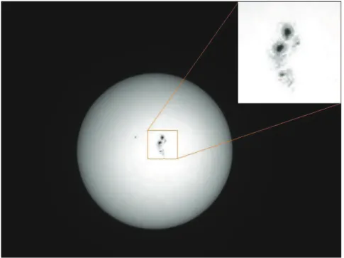
Sunspots are temporary phenomena on the surface of the Sun that appear as dark spots compared to surrounding regions. They are caused by intense magnetic activ-ity, which inhibits convection, resulting in areas of locally lower temperature. Al-though they are at temperatures of roughly 3,000–4,500 Kelvin, the contrast with the surrounding material at about 5,780 Kelvin leaves them clearly visible as dark spots, as the intensity of a heated black body (closely approximated by the photosphere) is a proportional toT4(whereTis the temperature in Kelvin). If the sunspot were isolated from its surroundings it would be blindingly bright. Sunspots expand and contract as they move across the surface of the sun and can be as large as 80×106 metres in diameter, making the larger ones visible from Earth with the naked eye (look at the Sun directly without a suitable filter at your peril, it can be done, but can also result in permanent burn blind spots on the retina). Spots often occur in groups (see Figure 1) which can rotate and mutate over time before disappearing. The earliest records of sunspots are of naked eye spots and occur in Chinese records from 364 BCE. Telescopic observation of sunspots date to 1610-11 when they were observed by Thomas Harriot, the Fabricius brothers, Christoph Scheiner and possibly others.
Similar spots on stars are commonly called starspots and both light and dark spots have been detected.
From early times sunspots have been used to measure the rotation rate of the Sun by in effect timing how long it takes a spot or group of spots to cross the Sun and reappear at the other edge. The first published measurement of the solar rotation rate was by Christoph Scheiner [2] who also noted that the apparent rotation rate was faster at higher solar latitudes. In what follows I will be doing this using a set of photos that I took in 2004 and using Gnumeric do to the data reduction.
The Data
MHF Journal Issue3
Figure 1: Detail of Sunspot Group 23th July 2004(Photo by the Author)
the Sun taken by the author between the 17th and the 23rd of July 2004. An example of such a photo is shown in Figure 1 (not strictly an example, the figure is a 4-frame integration of a sequence of photos taken in burst mode, the actual photos used where single frames). The photos where printed out, the centre of the sun on the image found and the distance of the a point midway between the two main spots in the group shown in Figure 1 from the centre measured. This allows us, with the assumption that the suns rotational axis is in the plane of the sky, to fit the data to a model which has unknown rotational period, time when the group first crossed the edge of the visible face of the Sun, and the groups solar latitude. In such a model the position of the group on the disk of the sun may be calculated:
x y =R cos(2π(t−t0)/T)cos(φ) sin(φ)
whereRis the radius of the solar disk in the image,φthe solar latitude of the sunspot group, t0 the time the group appeared at the edge of the visible disk, T the apparent period of solar rotation and t the time an image was captured. From this we may calculate the distance of the group from the centre of the image (and we don’t need to know the orientation of each image with respect to the Suns rotational axis). A montage of the images used is shown in Figure 2.
Then the model is fitted by adjusting the parametersφ,t0 andT to minimize the sum of the square error between the model prediction and the observed distance of of the group from the centre of the Sun. The estimated standard deviation for the measure-ment of the radial distance of the group from the centre of the solar image is about 2
MHF Journal Issue3
Figure 2: Montage of Photos of the Sun Taken(bottom right to top left)on the 17th, 20th, 21st, 23rd
and 24th of July 2004(rotated into approximately the same orientation).
mm. (Note technically the periodT was not used as a parameter rather the angular velocityω=2π/T was used)
The Spreadsheet Model
The Gnumeric spreadsheet implementing the model is shown in Figure 3. The main dialogs to set up the solver are shown in Figures 4,5 and 6
Results
The result of the fitting process can be seen in Figure 3. The least squares estimate for the solar rotation period is 27.3 days.
This is a point estimate and gives us no indication of the uncertainty in our estimate. It is not obvious how to calculate the error associated with our estimation process, so we revert to a Monte-Carlo technique. Assume that the solution found by the least squares procedure is close to the “true” solution, generate the distance from the edge of the Sun data corresponding to the times of the actual observations and then add in normally distributed errors with zero mean and SD equal to the estimated measurement SD in the real data. Use this simulated data to fit the rotation model and record the rotational period that is found. Repeat to generated a sample of rotational periods.
Doing this I generated a sample of 11 rotational periods with mean 27.46 days and standard deviation 1.15 days. From this we conclude that there is no significant evi-dence of bias in an estimate of rotational period generated the by the method we have used (the sample mean is only sightly more than 1 SD from the true rotational period in the Monte-Carlo experiment), and that for data similar to ours we expect a SD of ~1.2 days for our estimate of rotational period.
MHF Journal Issue3
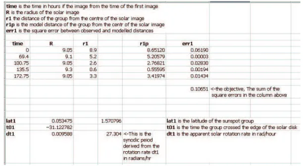
Figure 3: Gnumeric Spreadsheet with the data in the first three columns near the top and the model parameters on the left near the bottom(all distances in cm, times in hours)
Figure 4: Solver dialog to set the cell with the objective to minimize, and the cells that contain the parameters to be changed to find the minimum
MHF Journal Issue3
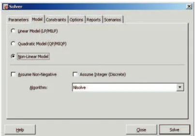
Figure 5: Dialog showing the solver method set to non-linear
MHF Journal Issue3
So our result is that we find the apparent rotational period of the Sun to be 27.3 days with a SD on this estimate of ~1.2 days. This is for a Sun spot group at a very low solar latitude (the solar period is latitude dependent increasing with latitude). This compares with the usually accepted value of 26.24 days for the equatorial rotational period of the Sun.
Assessment of the Gnumeric Solver
It is clear that Gnumeric and its solver performed satisfactorily for the task set it in this note. However several bugs made themselves apparent in the process:
• Constraints were not always observed
• The cell reference for the objective had the currently selected cell reference prepended every time that the solver dialog was called up
• A constraint with a numeric right hand side did not have the numeric value saved with the sheet
In addition there was no documentation that I could find that specified the optimiza-tion method that the solver implemented.
All three of the bugs I believe are in the known bugs data base on the Gnumeric site, and the second and possibly the third have been solved in the most recent release of Gnumeric. I expect that the documentation of the optimization algorithm will even-tually be corrected, there is a work around which involves examining the source code but this is not entirely satisfactory.
Compared to Excel the Gnumeric solver found a smaller minimum for the objective, but this did not result in a substantially different estimate of the rotational period. It is a limitation of spread sheets in general that without further automation (which is in principle possible) the number of Monte-Carlo replications achievable by hand cranking the model is limited by the patience of the analyst (in this case to 11 replica-tions). If a larger number of replications are needed it would be better to use a system designed for such purposes such as the numerical packages like Matlab, Euler, Octave, etc. However the learning curves for such tools are relatively steep for these tools and so the use of spreadsheets for teaching data analysis can be useful.
References
[1] Gnumeric Project:http://projects.gnome.org/gnumeric/
[2] Christoph Scheiner “Rosa Ursine sive solis”, book 4, part 2, 1630
[3] Wikipedia, “Sunspot”, http://en.wikipedia.org/wiki/Sunspot [accessed 9th August 2010]