A Lower Bound for Immersions of Real
Grassmannians
By
Marshall Lochbaum
Senior Honors Thesis
Mathematics
University of North Carolina at Chapel Hill
November 11, 2014
Approved:
Justin Sawon, Thesis Advisor Date
Abstract
The cohomology of the real Grassmann and flag manifolds is discussed at length, making use of Stiefel-Whitney classes. It is shown that the tan-gent bundle of the Grassmannian splits into line bundles over the flag manifold. Additionally, it is found that the cohomology of the flag mani-fold is exactly the polynomial algebraZ2[e1, . . . , en], for one-dimensional
classes ei, modulo the relationQi(1 +ei) = 1. Using facts about this
ring to compute the dimension of the Stiefel-Whitney class of the normal bundle to the Grassmannian, we find a lower bound for immersions of certain real Grassmannians. In particular,Gn Rn+k withn ≤2s ≤k andn+k≤21+scannot be immersed in dimension less thann 2s+1−1
.
1
Introduction
An immersion is a smooth map from one manifold into another whose derivative is injective at each point in the domain. Immersions are an important topic of study in the field of geometric topology, so it is natural to seek results on their existence or nonexistence. Here we consider immersions of the Grassmann manifoldsGn Rn+kinto Rl.
A significant amount of background material is provided here for the reader who is not familiar with details of the spaces involved or the notion of character-istic classes. This material is derived from Milnor and Stasheff [4] and comprises much of sections 1–3.
The main result of this paper is Theorem 5.2 showing thatGn Rn+kwhere
nandk satisfyn≤2s≤kandn+k≤21+scannot be immersed in dimension less thann 2s+1−1. This result is proved in [3], and the work here follows that paper closely (although it should be noted that Hiller and Stong writeGk Rk+n
rather than Gn Rn+k; the latter is used here to maintain consistency with
Milnor and Stasheff). We begin with a few standard results. First, the tangent bundle of Gn Rn+k is isomorphic to hom E, E⊥, where E is the universal
bundle whose fiber at a plane in the Grassmannian is that plane. Next, the immersion dimension of a manifold inRlmust be at least the dimension of the
manifold plus the dimension of the Stiefel-Whitney class of its normal bundle, which is the multiplicative inverse of the Stiefel-Whitney class of the tangent bundle. Last is thatw(T)w(E⊗E) =w(E)n+k, whereT =T G
n Rn+kis
the tangent bundle of the Grassmannian.
Along the way we will use the flag manifold Flag(Rn), whose elements are
strictly increasing sequences of linear subspaces ofRn. The relevant property
is that the universal bundleE pulls back to a direct sum of line bundles under the projection Flag Rn+k → Gn Rn+k sending a flag to its n-dimensional
2
The Grassmann manifold
The Grassmann manifold, or Grassmannian, of dimension n over Rn+k, is a
manifold whose elements are the linear subspaces ofRn+k of dimensionn. It is
denotedGn Rn+k.
2.1
Topology
To produce the topology onGn Rn+k, it is most convenient to define it as a
quotient space.
Definition 2.1. The Stiefel manifold1 Vn Rn+k is the space of all linearly
independent ordered sets (“n-frames”) ofn vectors inRn+k. It is topologized as a subspace ofRn(n+k)=M(n+k, n), consisting of those matrices all of whose
n×nminors have nonzero determinant.
Vn Rn+k is the preimage of (R\ {0})(
n+k
n ) under the function sending a
matrix to a list containing for each choice ofnofn+kcolumns the determinant of those columns. That function is continuous (in fact, it is a polynomial), so Vn Rn+kis an open subset ofRn(n+k).
Definition 2.2. The GrassmannianGn Rn+kis the set ofn-dimensional
lin-ear subspaces ofRn+k, with the quotient topology derived from the map from
Vn Rn+ktoGn Rn+ksending each set of vectors to the space it spans.
For convenience, we setG=Gn Rn+kandV=Vn Rn+kfor the
remain-der of this section.
It is clear from this definition that the spaces G1 R1+k are identical to RPk, asV1 R1+kis justR1+k\ {1}, and 1-dimensional subspaces are lines.
Theorem 2.1. Gn Rn+kis compact and Hausdorff.
Proof. The quotient map V → G factors through a map from V to the set V0
n Rn+k
(or V0) oforthonormal n-frames given by the Gram-Schmidt
pro-cedure. ThusGcan be represented as a topological quotient of V0, with the
subspace topology inherited from S(n+k)−1n
. As that space is compact and V0is closed in it (being the preimage ofI∈M(n,R) under the mapA7→ATA),
Gis compact.
To show that Gis Hausdorff, it suffices to find a continuous function sep-arating two given elements X, Y in G. Letw ∈X \Y, and definef(Z) to be the square of the distance fromwtoZ∈G(in the Euclidean metric onRn+k).
Thus
f(Z) =w·w−πZ(w)·πZ(w)
=w·w+X
i
(zi·w)
2
,
1This definition is not universal: many sources define the Stiefel manifold as the space of
where πZ is projection onto Z and {zi} n
i=1 is any orthonormal basis for Z.
Clearlyf(X) = 0< f(Y), and the above formula shows that the induced map is continuous onV0 and hencef is continuous onG.
2.2
Topological manifold structure
We will now demonstrate that any pointX ∈Ghas a neighborhood
U =Y ∈G|Y ∩X⊥={0} ,
which is homeomorphic to the real vector space hom X, X⊥. This proves that Gis a topological manifold of dimension
dim hom X, X⊥
= dimX·dim X⊥
=nk.
LetY ∈U for the neighborhoodU described above. Thus
Y ⊂Rn+k=X⊕X⊥.
Define orthogonal projectionsp:Rn+k→X,q:
Rn+k→X⊥. Thusp(Y) =X,
and since dimY = dimX, p|Y is a linear isomorphism. Then the map
q◦(p|Y)−1:X →X⊥
is a function in hom X, X⊥
corresponding toY. Conversely, such a function yieldsY, which is its graph: givenf:X →X⊥,
Y ={x+f(x)|x∈X}.
The resulting mapY →hom X, X⊥
is continuous: choose a frame{xi} n i=1
for X (that is, an element in V that maps to X). For any Y ∈ U, (p|Y)−1 sends the chosen frame to a frame on Y, yielding an injective mapλ from U
to V with inverse given by the canonical projection back to G. This map can be shown to be continuous through explicit calculation (noting that λ is continuous if and only if the induced mapV→Vis continuous). Given any set ofnvectors{vi}
n
i=1, there is a linear mapX →Rn+k sendingxi tovi. Clearly
the assignment of linear maps to sets of vectors is linear invi, and so when we
restrict to Im(λ) ⊂ V we obtain a linear map—call it µ. Finally, there is a continuous function from hom X,Rn+kto hom X, X⊥given by composition
withq, the projection ontoX⊥. Thus Φ is given by the composition
U λ //V µ //hom X,Rn+k
q◦ //
hom X, X⊥
and is continuous since each component is continuous. The inverse map from hom X, X⊥
to U is also continuous, as choosing a frame{xi}
n
i=1 for X yields a frame{yi} forY which depends continuously on
a function f: X → X⊥, with yi = xi+f(xi). Thus we have constructed a
2.3
Smooth structure and tangent bundle
To show that G is a smooth manifold, it suffices to show that the maps Φ obtained at each point inGare smoothly compatible. ConsiderXandU defined as before, and letX0 ∈U. X0 has a neighborhood U0, with a homeomorphism Φ0:U0 →hom X0, X0⊥
. A straightforward computation shows that Φ and Φ0 are smoothly compatible, that is,
Φ0◦Φ−1: Φ(U∩U0)→Φ0(U∩U0)
is smooth.
Definition 2.3. The universal bundleE onGn Rn+kis the subbundle of the
trivial bundleRn+k obtained by taking at each point inG
n Rn+kthe subspace
it corresponds to.
We also defineE⊥'Rnk/Eto be the subbundle ofRn+kobtained by taking
the vector spaceX⊥ to be the fiber overX∈G.
Then, because the fiber ofEoverX isX and the fiber ofE⊥ overX isX⊥, the tangent space ofGis given by
T 'hom E, E⊥ (1)
as a vector bundle.
3
Stiefel-Whitney Classes
3.1
Definition and basic properties
The Stiefel-Whitney class w(V) of a finite rank real vector bundle V over a space X is an element of H∗(X;Z2). We write w(V) = Li∈Nwi(V), where wi(V)∈Hi(X;Z2). The operationwuniquely satisfies:
1. Normalization.
w γ11
= 1 +a
Whereγ1
1 is the tautological line bundle overRP1 andais the generator
ofH1 RP1;Z2
, so thatH∗ RP1;Z2
=Z2[a]/ a2
.
2. Rank.
w0(V) = 1∈H0(X;Z2)
wi(V) = 0∈Hi(X;Z2), if i >rank(V).
3. Whitney product formula.
4. Naturality.
w(f∗V) =f∗w(V)
forf∗ the pullback by a continuous mapf:X0→X.
Proofs of the existence and uniqueness of the Stiefel-Whitney classes are given by Milnor and Stasheff [4].
It is clear from the last axiom that given a homeomorphism of spaces, the induced isomorphism in cohomology fixes Stiefel-Whitney classes. Addition-ally we see that the trivial bundle Rn over a space has Stiefel-Whitney class
zero, since it pulls back from the trivial bundle on a point, which has trivial cohomology.
In the case of Grassmannians, it can be shown that the cohomology ring is generated by the Stiefel-Whitney classes wi(E), 0 < i≤n, of the universal
bundle. We refer to again Milnor and Stasheff for a proof [4, p. 83].
3.2
Computation for
T
(
RP
n)
For the real projective space RPn = G1 Rn+1, the universal bundle has
di-mension one and hence has just one nonzero Stiefel-Whitney class,w1(E) =a.
Thus the cohomology ring is a quotient of the ring Z2[a]. As the projective
space must have a top-level cohomology class, but no classes of greater degree, its cohomology ring isZ2[a]/ an+1
(this fact can be shown by more elementary means, but Stiefel-Whitney classes provide a very elegant proof). We will refer to the universal bundle E onRPn as the tautological line bundleγ to match
convention.
As an aside, it is simple to compute w(γ) using only the knowledge of
H∗(RPn;
Z2). Let the tautological bundle onRP1beγ1. The inclusionR1→Rn
induces an inclusion ι:RP1 →
RPn. ι∗ pullsγ back to theγ1, whose
Stiefel-Whitney class we know from axiom 1. By naturality,ι∗(w(γ)) =w(γ1) = 1 +a,
implying thatw1(γ) is nonzero. Sincew(γ) has no terms of degree greater than
one, asγis a one-dimensional bundle, we havew(γ) = 1 +a.
We now complete our computation ofw(T(RPn)), starting with equation 1:
T(RPn)'hom γ, γ⊥.
To simplify, we add the trivial bundleR= hom(γ, γ) to each side, obtaining
T(RPn)⊕R'hom γ, γ⊥⊕γ
= hom γ,R1+n
= hom(γ,R)⊕1+n.
We can further simplify using the fact that hom(γ,R) =γ, from Appendix A. Applyingwand using the Whitney product formula,
w(T(RPn))w(R) =w(γ)1+n.
Sincew(R) = 1, we obtain
3.3
Consequences for immersions
Suppose we have a manifoldM of dimensionnand an immersion
f:M →Rn+k.
Thenf∗ sends T Rn+k
to a vector bundle on M, which is necessarily trivial of dimensionn+k and contains T(M) as a sub-bundle. Defining the normal bundle
N(M) =T(M)⊥
as a sub-bundle of the trivial bundleRn+k, we have
N(M)⊕T(M) =Rn+k
and consequently
w(N(M))w(T(M)) =w Rn+k
= 1.
If we know the cohomology ring ofM and the Stiefel-Whitney class of its tan-gent space, this places constraints on the dimension of spaces in which M is embedded. The constraints are due to the fact that the dimension ofN(M) is
k, so that terms of order greater thankmust be zero. If k≥n, then there are no restrictions as the cohomology ring ofM has no terms of order greater than
k.
3.4
Stiefel-Whitney class inverses
The cohomology ring H∗(M;
Z2) of a space M is a graded algebra over Z2.
We consider only spaces M with finite-dimensional cohomology. Let A =
H∗(M;Z2) andAi =Hi(M;Z2), so that
A=
n
M
i=0
Ai.
Letπi be projection ontoAi, that is, ifa=Piai withai∈Ai, thenπi(a) =ai.
The Stiefel-Whitney classes occupy a subset W of A with constant coefficient equal to one,
W ={w∈A|π0(w) = 1}.
We will show that this set is a group under multiplication, and consequently that we can divide as well as multiply the Stiefel-Whitney classes of tangent bundles.
Define the index functioni:A→[0,∞] by
i(0) =∞
Clearlyi(a+b)≥min(i(a), i(b)), andi(a)> nonly if a= 0. It is easy to show additionally thati(ab)≥i(a) +i(b).
To show thatW is closed under multiplication, let 1 +v,1 +w∈W. Then
(1 +v)(1 +w) = 1 +v+w+vw
i((1 +v)(1 +w)−1)≥min(i(v), i(w), i(v) +i(w))≥1,
so (1 +v)(1 +w) lies in W. W clearly contains the multiplicative identity 1, and we can demonstrate that it has inverses using the formula
1
1 +x= 1 +x+x
2+x3+· · ·
where factors of−1 are omitted because Ais aZ2-algebra. Sincei(x)≥1, we
havei xk
≥k, so xk is zero forklarger than the maximum graden. Then
(1 +x) 1 +x+x2+· · ·+xn
= 1 +xn+1= 1.
ConsequentlyW is a group under multiplication and the inverse formula given provides the unique inverse. This inverse is unique not only in W but in A
because ifa(1 +w) = 1 for a∈ A, 1 +w∈W, then π0(a)π0(1 +w) =π0(1),
or π0(a) = 1. For a Stiefel-Whitney class w(V), we denote its multiplicative
inverse byw(V).
3.5
Immersions of projective spaces
We combine the results of the two previous sections:
Theorem 3.1. A lower bound for the immersion dimension ofn-dimensional manifoldM isn+k, where
k= dimw(N(M)) = dimw(T(M)).
We now specialize to the case of RPn, with H∗(RPn;Z2) = Z2[a]/ an+1
andw(T(RPn)) = (1 +a)n+1.
We note that in any algebra overZ2, (a+b)2=a2+b2, that is, squaring is a
homomorphism. We conclude that (1+a)2l = 1+a2l, which is 1 inZ2[a]/ an+1
if 2l > n. Therefore the inverse of w(T(RPn)) = (1 +a)n+1 in H∗(RPn;Z2) is
(1 +a)2l−n−1, where 2l> n. This polynomial has the same value for alll that
satisfy the given inequality by uniqueness of inverses. Its degree is computed most easily if we additionally require that 2l≤2n, so that 2l−n−1< nis the
degree. Consequently
Theorem 3.2. The spaceRPncannot be immersed in dimension less than2l−1,
4
The flag manifold
4.1
Definition
In working with the Grassmannian it is convenient to introduce another quotient of V0
n(Rn), the space of orthogonal n-frames inRn. Our intention is for the
flag manifold, which we denote using Flag(Rn), to consist of all complete flags
inRn, that is, all strictly increasing sequences
{0}=V0(V1(V2(· · ·(Vn=Rn.
As the dimensions of theVimust be strictly increasing, it follows that dimVi=i.
Noting that a flag is equivalent to an ordered set of orthogonal lines inRn (so
thatVi is the span of the firstilines), we let
Definition 4.1. The flag manifold Flag(Rn) is the quotient ofV0
n(Rn) by the
relation setting{xi} n i=1∼ {x
0
i} n
i=1 whenxi=±x0i for alli.
Thus the flag manifold is the quotient of the action onV0
n(Rn) of a discrete
group (Z×)n, whereZ× ={−1,1}under multiplication (soZ× is cyclic of order 2). V0
n(Rn) is the submanifold of Sn−1
n
⊂M(n,R) satisfying the (smooth) relationATA=I, so Flag(
Rn) inherits its smooth manifold structure.
The flag manifold Flag Rn+kprojects to the GrassmannianGn Rn+kby
sending a flag to itsn-dimensional space.
4.2
Cohomology
Theorem 4.1. The cohomology ring H∗(Flag(Rn);
Z2) is generated byn one-dimensional classese1, e2, . . . , en, which obey the relation
n
Y
i=1
(1 +ei) = 1.
Proof. The desired classes are found using the mapπ: Flag(Rn)→
RPn−1
n
which sends a flag to the orthogonal lines defining it. The cohomology ring of each copy ofRPn−1is generated by a single one-dimensional class, and we define
ei to be the pullback of this class in theith copy.
By naturality of Stiefel-Whitney classes, we have
ei=π∗i(w1(γ)) =w1(πi∗(γ)),
where πi is the projection of Flag(Rn) onto the ith component. We let γi =
πi∗(γ). The bundle L
iγi is the trivial bundleRn, since the product of all the
lines in a flag is always the entire space. The relation of the classes,Q
i(1 +ei) =
1 is then given by applyingw.
Theorem 4.2. Let E be a fiber bundle over the space B with fiber F and projection mapp:E→B, andR be a commutative ring. Assume also:
(a) Hn(F;R) is a finitely generated freeR-module for each n.
(b) There exist classes cj ∈ Hkj(E;R) such that i∗(cj) form a basis for
H∗(F;R)for each inclusion i:F →E sendingF to a fiber.
Then the map Φ :H∗(B;R)⊗R H∗(F;R) → H∗(E;R), Pijbi ⊗i∗(cj) 7→
P
ijcj^ p∗(bi) is an isomorphism.
Flag(Rn) may be viewed as a tower of fiber bundles where the fiber in each
case is a projective space. We can obtain this tower by successively choosing subspaces ofRn—firstV1, thenV2, and so on. LetFk be the space of flags
{0}=V0(V1(· · ·(Vk
where dimVk =k. Clearly our choice for V1 is any line inRn, so F1 is equal
toRPn−1, or equivalently a fiber bundle over a single point with fiber
RPn−1.
Once we have chosen the firstk−1 subspaces, the choice ofVk is equivalent to
picking a line inRn/V
k−1, which is isomorphic to Rn−k+1, meaning thatFk is
a fiber bundle overFk−1 with fiberRPn−k.
Given the fiber bundleFk→Fk−1, we verify the conditions for Leray-Hirsch
(with R = Z2). Since the cohomology ring of the fiber, H∗ RPn−k;Z2, is
equal toZ2[a]/ an−k+1
, each cohomology groupHj
RPn−k;Z2
is the freeZ2
-module generated byaj. To generate the group, then (and satisfy condition b),
it suffices to show thati∗(ek) is nonzero inRPn−k (equivalently, it is equal to
a). But this follows becauseπ◦i is the natural inclusion induced by the map
Rn−k →Rn, so it sends the generator ofRPn to the generator ofRPn−k.
This construction makes it clear that a set of elements which generate
H∗(Flag(Rn);Z2) by addition is given by the products Qiekii satisfying ki ≤
n−1 for all i. It happens that the relation Q
i(1 +ei) = 1 allows us to write
any polynomial inei in terms of such monomials, a fact which we do not prove
(or require) in this paper.
4.3
Monomials in
H
∗(Flag(
R
n);
Z
2)
Theorem 4.3. In the cohomology ofFlag(Rn),(1) eni = 0 for alli.
(2) The top dimension is 12n(n−1). A monomialQ
ie ki
i of that dimension is
nonzero if and only if theki are a permutation of the set{0,1, . . . , n−1}.
Proof. (1) is clear simply by noting that ei = π∗i(a), where a generates the
cohomology ofRPn−1. In the latter space,an= 0, soen
i =πi∗(an) = 0.
To show (2), we begin with the above construction of the flag manifold as an iterated fiber bundle. This construction clearly indicates that
dim(Flag(Rn)) =
n
X
k=1
dim RPn−k=
n−1
X
i=0
i=n(n−1)
That the given monomial is nonzero is readily apparent from Leray-Hirsch. For simplicity, we go through theeiin order. The top-dimensional component added
at each step is eni−i, so the product of this element and the previous nonzero component is the top-dimensional component in the new flag manifoldFi. Since
the cohomology ring ofF0(a point) is trivial, the termQ
n i=1e
n−i
i is nonzero.
There is a map Flag(Rn) → Flag(
Rn) for any permutation σ ∈ Sn which
sends a tuple of orthogonal lines to the same lines permuted byσ. Clearly such a map is a homeomorphism. However, this map also rearranges the cohomology classes by sending ei to eσ(i). Consequently the monomial Qie
n−i
σ(i) for any
σ∈Snis nonzero, or equivalentlyQie ki
i is nonzero if thekiare a rearrangement
of the set{0,1, . . . , n−1}.
It remains to show that any monomial with dimension 12n(n−1) not of this form is equal to zero. We will call monomials fitting the form, that is,
Q
ie ki
i with {ki} = {0,1, . . . , n−1}, decreasing monomials. For an arbitrary
top-dimensional monomial expressed as a productQ
ie ki
i , letKj, for 0≤j≤n,
be the set of basis elementsei for which the correspondingki are greater than
or equal toj. Definedj=|Kj|andpj=Qi∈Kjei, so that
P =
n
Y
j=1
pj.
Clearly Kj ⊂ Kj−1 for all j, so dj form a non-increasing sequence. For a
decreasing monomial, we have dj = n−j, and the sequence (dj) is strictly
decreasing. In fact this property holds only for decreasing monomials: the total dimension of the monomial is
X
j≥1
dj=
X
k
d0−
n
X
j=1
dj−dj−1
,
where d0 is fixed at n. The maximal value of this expression is attained only
whendj−dj−1is minimized, that is, when it is always equal to 1.
We will show that monomials which are not decreasing are zero by directly using the relation found in Theorem 4.1,
n
Y
i=1
(1 +ei) = 1.
For j > 0, the degree j component of the left-hand side is the sum of all j -dimensional monomials which contain at most one copy of each ei. Thus it
contains nj components corresponding to the choices of j of the ei. As the
jth component of the right-hand side is zero, that polynomial is zero in the
cohomology ring of Flag(Rn), or in other words a product ofjdistinct generators
is equal to the sum of all other products ofj distinct generators. As a special case, we note that the productQn
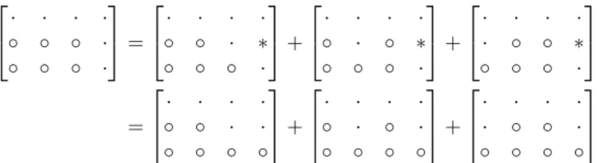
· · · · ◦ ◦ ◦ · ◦ ◦ ◦ · = · · · · ◦ ◦ · ∗ ◦ ◦ ◦ · + · · · · ◦ · ◦ ∗ ◦ ◦ ◦ · + · · · · · ◦ ◦ ∗ ◦ ◦ ◦ · = · · · · ◦ ◦ · · ◦ ◦ ◦ ◦ + · · · · ◦ · ◦ · ◦ ◦ ◦ ◦ + · · · · · ◦ ◦ · ◦ ◦ ◦ ◦
Figure 1: Rewriting a monomial as a sum of vanishing terms. The rows corre-spond toplwithp1at the bottom, and the columns to variablesei, with element
(l, i) marked ifei∈Kl. Each monomial in the final sum is zero since it contains
ei for eachi.
Suppose we have a monomial P = Q
ie ki
i for which the first (that is, for
minimal j) value of dj −dj−1 not equal to 1 is 0. We will demonstrate by
induction that such monomials are zero. Ifj = 1, this is clear, asd1 =d0=n
implies that the p1 contains ei for each 1 ≤ i ≤ n, and thus is the product
of all generators, which we have just noted is zero. Now suppose j > 1. By hypothesis dj = dj−1, so Kj = Kj−1 and pj = pj−1. Now rewrite pj as the
sum of all other products ofdj generators (this procedure is illustrated in figure
1). Consider a single summandP0of the resulting expression forP obtained by replacingpj with qj =Qea∈Ljea. Since Lj is distinct from Kj =Kj−1, some
termsea∈Ljare not inKj−1. Consequently for each such termea, there is an
la < j−1 such that ea ∈Kla\Kla−1. Thela are distinct, since the fact that dl−dl−1= 1 forl < jimplies that Kla\Kla−1 has only one element, and the ea are distinct. Then takingl = minala, we havedk−dk−1 = 1 for allk < l,
whiledl−dl−1= 0, and P0 is zero by induction onj.
To complete the proof, consider the monomials for which the first value of
dj −dj−1 not equal to 1 is greater than one. We will show that each such
monomial is zero in two steps—first, by assuming that dj −dj−1 is exactly
2, and next, by showing that any monomial with a greater difference can be rewritten as a sum of monomials of the first kind. To simplify both proofs, we note a consequence of the result from last paragraph on the rewriting operation performed there: when rewriting a term pl of P, we can ignore combinations
not contained entirely in Kj−1. This is due to the fact that if any ei in the
result falls outside of that set, then the firstdj−dj−1not equal to 1 is equal to
0, so the resulting monomialP0 is zero. We also define the function
h(P) =X
l
ldl,
a positive integer associated to any given monomial. If we choosekwithKk =
Kk−1, and rewritepk, then each summand P0 in the result must have lower h
thanP. This is because some term ofLk(wherepk is moved toQea∈Lkeamust
hbyk−l. No termKlwithl > kcan increase in size when we rewrite, because
any element ofLk inKl merely fills the value occupied earlier by an element of
Kk. Thush(P)> h(P0).
Let dj−dj−1 = 2, and dl−dl−1 = 1 for l < j. Choose k > j such that
dk −dk−1 = 0 (recall that we are guaranteed at least one such index because
the monomial is not a decreasing one). When we rewritepk, the terms ˜pkwhich
lie entirely inKj−1fall in one of the following categories:
• Two elements of ˜pk lie in Kj\Kj−1. In this case, the correspondingP0
will haveKj0 =Kj0−1 and be zero.
• Exactly one element lies in Kj \Kj−1. In this case, there is another
term which contains the other element and is otherwise equal. These elements are equal, as when we rewritepjin the first, the only combination
contained inKj−1is thepj of the second. Thus they annihilate.
• All elements of ˜pk lie in Kj−1. Here we use the fact that h(P)> h(P0)
(noting that we rewrote a term pk = pk−1). As there is a minimum
possibleh,P0 is zero by induction onh.
Now letdj−dj−1>2. Again, we choose k > j withdk−dk−1= 0, rewrite
pk, and split the terms contained inKj−1 into cases:
• The elements of ˜pk coverKj\Kj−1. Again, we obtainP0 = 0 asKj0 =
Kj0−1.
• The elements of ˜pkcover all but one ofKj\Kj−1. Now we havedj−dj−1=
1, butd0j+1≤dj, sod1+0 j−d0j≤2. ThusP0is not a decreasing monomial,
andh(P)> h(P0).
• The elements of ˜pk leave at least two elements of Kj\Kj−1 uncovered.
ThenP0 is not a decreasing monomial, andh(P0)< h(P).
To summarize, each monomial which is non-decreasing is either zero or can be written as a sum of non-decreasing monomials with strictly smallerhvalue. Sincehis a positive integer, all non-decreasing top-dimensional monomials are zero.
Remark. The rewriting procedure described in the above proof can also be used to show explicitly that all decreasing monomials are equivalent. LetP be the decreasing monomial given by the permutationσ∈Sn, that is,
P=
n
Y
i=1
eiσ−(i1), pj=
Y
i>j
eσ(i), Kj =
eσ(i)|i > j .
Then when we rewritepj, the only terms that give a decreasing monomial are
those whose elements lie in Kj−1 (as discussed above) but cover Kj+1. The
latter condition arises because if an element of Kj+1 is left out, that element
evident that the only polynomial satisfying these conditions other thanpjis the
one that exchangeseσ(i) for eσ(i−1). Since the exponents of those terms differ
only by one, this exchange also exchanges the two terms in the full monomial, so that the new monomial is the one given byσ◦(j−1, j). SinceSnis generated
by the pair-exchanging permutations (j−1, j), we can obtain all the decreasing monomials using transformations of this form.
5
Immersions of Grassmannians
5.1
The Hsiang-Szczarba formula
This section follows closely the derivation in section 3.2. To compute the Stiefel-Whitney class of the tangent bundleT of Gn Rn+k, recall (from equation 1)
that
T 'hom E, E⊥
,
whereE is the universal bundle. Adding hom(E, E) to both sides,
T ⊕hom(E, E)'hom E, E⊥⊕E
= hom E,Rn+k
= hom(E,R)⊕n+k.
SinceGn Rn+kis compact and Hausdorff,
hom(E,R) =E∗'E.
We then obtain, by taking Stiefel-Whitney classes of the earlier equation,
w(T)w(E⊗E) =w(E)n+k. (2)
This result is sometimes referred to as the Hsiang-Szczarba formula. We know thatw(E) = 1 +P
ixi, wherexi generateH∗ Gn Rn+k;Z2
as a ring. It remains to findw(E⊗E).
5.2
The splitting principle
The Stiefel-Whitney class of a tensor product is not readily apparent in the general case. However, there is a simple formula for line bundles: given line bundlesL1, L2, with w(L1) = 1 +l1 andw(L2) = 1 +l2, we have
w(L1⊗L2) = 1 +l1+l2.
This is equivalent to a proposition from Hatcher’sVector Bundles and K Theory, which states that the function w1: Vect1(X) → H1(X;Z2) is a group
For general vector bundles, the splitting principle provides a convenient way to calculate tensor products. The principle states that for any spaceX with vector bundleV, there is a spaceY and mapp: Y →X such that the induced homomorphismp∗on cohomology is injective and the vector bundle p∗V splits as a direct sum of line bundlesp∗(V) =Ln
i=1Vi. Then given a vector bundle
V, the following procedure suffices to computew(V ⊗V): first select a spaceY
and mapp:X →Y with the above properties and splitp∗V into a sum of line bundlesVi. Computew(Vi) = 1 +vi. Then
p∗(w(V ⊗V)) =w(p∗(V ⊗V)) =w
M
i
Vi
!
⊗ M
i
Vi
!!
=w
M
ij
Vi⊗Vj
=Y
ij
w(Vi⊗Vj)
=Y
ij
(1 +vi+vj).
Assuming we are working inZ2, we can simplify slightly, noting that 1+vi+vi =
1 and (1 +vi+vj)2= 1 +vi2+v2j. We obtain
p∗(w(V ⊗V)) =Y
i<j
1 +v2i +v2j
.
Finally, we must find a cohomology class whose value underp∗is the computed result. Such a class will necessarily be equal tow(V ⊗V) sincep∗ is injective.
We will not need to prove, or in fact use, the splitting principle in order to carry out this procedure, as it turns out we know a space over which the vector bundleE splits—it is the flag manifold discussed in section 4.
Theorem 5.1. The map Ψ : Flag Rn+k →Gn Rn+k sending a flag to the
plane in it of dimensionnsplits the universal bundle into line bundles.
Proof. Recall the mapπ: Flag Rn+k→ RP(n+k)−1
n+k
sending a flag to the tuple of orthogonal lines associated with it. Composingπwith projection onto theith factor yieldsn+kmapsπi: Flag Rn+k→RP(n+k)−1. We claim that
Ψ∗(E) =
n
M
i=1
πi∗(γ)
whereγis the tautological line bundle onRP(n+k)−1. But this is clear: the fiber
of Ψ∗(E) at a flag containing the planeVnis simply that plane, and the fiber of
the direct sum is the direct sum of the linesV1, V2/V1, . . . , Vn/Vn−1, also equal
We also need to demonstrate that Ψ∗ is injective on cohomology, a fact we will show using the Leray-Hirsch theorem. The isomorphism given in the conclusion of that theorem automatically implies that p∗ is injective on coho-mology, since p∗(b) = Φ(b⊗1). Thus we need only find a sequence of fiber bundles with initial base spaceGn Rn+kand final space Flag Rn+keach
sat-isfying the conditions of Leray-Hirsch, and for which the resulting projection Flag Rn+k
→ Gn Rn+k is Ψ. For the first such map, we recall the
par-tial flag manifold Fn from the proof of Theorem 4.1. This manifold may be
represented as a bundle overGn Rn+k where psends a partial flag to its n
-dimensional component. The fiberp−1(Vn) for a plane Vn ∈Gn Rn+kis the
set of partial flags ending inVn, a space which is isomorphic to Flag Rn−1via
any isomorphism of Vn and R. The remainder of the fiber bundles to get to
Flag Rn+kare simply those constructed while proving Theorem 4.1, which we
verified in the proof to satisfy Leray-Hirsch. Thus we need only show that the first fiber bundle satisfies those conditions. Condition (a) is immediate because
H∗(Fn;Z2) is a polynomial ring, and condition (b) follows by taking the classes
ei for 1 ≤ i ≤ n−1 in Fn as generators for Flag Rn−1. Clearly the total
projection sends a flag in Flag Rn+k
to itsn-dimensional component, that is, it is exactly Ψ. Thus Ψ∗ is injective on cohomology.
5.3
An immersion bound for some Grassmannians
In this section we will combine the Hsiang-Szczarba formula with our earlier work on the flag manifold and some extensive computation to conclude:
Theorem 5.2. Given n, k such that n≤2s≤kandn+k≤2s+1,G
n Rn+k
cannot be immersed in dimension less thann 2s+1−1
.
Whenn= 1 this result restricts to the bound of Theorem 3.2 on projective spaces. To prove it we begin with
Lemma 5.3. In any Z2-algebra generated by one-dimensional classes ei, 1 ≤
i≤n, the identity
Y
1≤i<j≤n
(ei+ej) =s(n−1,n−2,...,1)(e1, . . . , en)
holds, wheresis a monomial symmetric polynomial as defined in Appendix B.
Proof. Forn= 2, the result is clear, as the left-hand side has only a single term
e1+e2and the right-hand side is equal tos(1)(e1, e2) =e1+e2, the sum of the
two monomials with degree one.
Now for a givenndenote the left-hand side by An. Assume
An =s(n−1,n−2,...,1)(e1, . . . , en).
ThenAn+1 is formed by multiplyingAn by all the terms containingen+1:
An+1=An n
Y
i=1
The 2n terms in the product can be divided according to the number of times
en+1 appears in them. In each case, the remaining ei in that term are distinct
and taken from the set{1, . . . , n}. Thus we have
n
Y
i=1
(ei+en+1) =
n
X
j=0
ejn+1s(1,...,1)(e1, . . . , en),
where the s(1,...,1) term on the right-hand side contains n−i ones. In order
to multiply this result by An, we move An inside the sum, and use Corollary
B.2’s statement that the products(1,...,1)(e1, . . . , en)·s(n−1,n−2,...,1)(e1, . . . , en)
is equal tos(n,n−1,...,j+1,j−1,...,0)(e1, . . . , en). Thus
An+1=
n
X
j=0
ejn+1s(n,n−1,...,j+1,j−1,...,0)(e1, . . . , en).
But the sum on the right simply groups all of the monomial components of
s(n,n−1,n−2,1,...,0)(e1, . . . , en+1) by the number of copies ofen+1 they contain, so
it is equal to that polynomial. The lemma now follows by induction.
Lemma 5.4. wn(n−1)(E⊗E)is nonzero inH∗ Gn R2n−1;Z2. Proof. Since the map Ψ : Flag R2n−1
→Gn R2n−1induces an injective map
Ψ∗ in cohomology, it suffices to show that then(n−1)-dimensional term of
Ψ∗(w(E⊗E)) = Y
1≤i<j≤n
1 + (ei+ej)
2
,
whereeiare the generators ofH∗ Flag R2n−1;Z2
, is nonzero. The number of
terms in the product is 1 + 2 +· · ·+ (n−1) = n(n2−1), so the term of dimension
n(n−1) includes no 1 terms of the product and is equal to
Ψ∗ wn(n−1)(E⊗E)
= Y
1≤i<j≤n
(ei+ej)
2
= s(n−1,n−2,...,1)(e1, . . . , en)
2
=s(2n−2,2n−4,...,2)(e1, . . . , en)
(where for the last equality we recall that squaring is a homomorphism). To show that this term is nonzero, we multiply by the value
e=e2e23· · ·e
n−2
n−1e
n−1
n e n−2
n+1· · ·e2n−2.
One term in the product is
e·e21n−2e22n−4· · ·e2n=e21n−2e22n−3· · ·e2n−2.
Because the product is homogeneous and this term has degree 12(2n−1)(2n−2), the dimension of Flag R2n−1, we can apply the second fact from Theorem 4.3
Each term in the product is obtained from an assignment of values in the tuple (2n−2,2n−4, . . . ,0) to indices 1, . . . , n. We will demonstrate that the only ordering which yields a nonzero product is the one placing them in descending order. The result follows from induction on the tuple index: to begin, no term can have degree higher than 2n−2, so the exponent 2n−2 must be paired withe1, which has exponent 0 (the minimum) in e. Next, no remaining term
can have degree higher than 2n−3, so 2n−4 must be sent to index 2, with exponent 1, the new minimum. Each time we add the term 2n−2j at index
j in the tuple, the maximum exponent of any remaining ei is 2n−j−1 and
the minimal remaining exponent ineis the one forej,j−1. The sum of these
exponents is 2n−j−1, so thejth exponent in the tuple must be paired with
ej. Because Ψ∗ wn(n−1)(E⊗E)
yields a nonzero monomial when multiplied bye,wn(n−1)(E⊗E) is nonzero as desired.
Lemma 5.5.Leti:Gn Rn+k−1→Gn Rn+kbe the natural inclusion sending
a plane X ⊂ Rn+k−1 to X × {0} ⊂ Rn+k, and consider an arbitrary class
x∈Hn(k−1) G
n Rn+k;Z2
. Then
x ^ wn(E),
Gn Rn+k=i∗(x),Gn Rn+k−1,
where[M] is the fundamental class of the spaceM.
Proof. The proof here is substantially the same as that of [5]. The result arises from the construction of Flag Rn+k
as an iterated fiber bundle overGn Rn+k
illustrated in Theorem 5.1. If we decompose the fiber Flag(Rn) of the first
bundle into an iterated bundle of projective spaces RPn−1,RPn−2, . . . ,RP1,
then we obtain a representation of Flag Rn+k as an iterated fiber bundle
over Gn Rn+k all of whose fibers are projective spaces. Lettingu be a
top-dimensional form in the Grassmannian (and also its pullbacks into bundles over the Grassmannian, for simplicity), the top-dimensional forms in the resulting bundles over the Grassmannian are
uen1−1, uen1−1en2−2, uen1−1en2−2en3−3, . . .
for the first set of bundles. Then ifu0 denotes the last of these (and pullbacks, again), the top-dimensional forms leading to Flag Rn+kare
u0ekn−+11, u0ekn−+11enk−+22, u0ekn−+11enk−+22ekn−+33, . . . .
Note thatendoes not appear in any of the above expressions. This is because the
nthplane of a flag in Flag
Rn+kis already determined by the Grassmannian—
indeed, it is the plane given by the projection Ψ—so any factors of en come
from the Grassmannian. We may include a fiber bundle for thenth plane, but
its fiber will beRP0, a single point. From the above, the top-dimensional form
derived fromuis
Ψ∗(u)en1−1e2n−2. . . en−1ekn−+11e
k−2
This class must have the same value onFlag Rn+kasuonGn Rn+k.
To obtain our result, first consider
i∗(x),
Gn Rn+k−1. This expression
is equal to the value of
Ψ∗(i∗(x))enn−1. . . en−1ekn−+11. . . en+k−2
on Flag Rn+k−1, where Ψ∗◦i∗(x) = (i◦Ψ)∗(x) is a symmetric function of
en+1, . . . , en+k−1. The left-hand side
x·wk(E),
Gn Rn+k is given by the
value of
Ψ∗(x)e1. . . en·enn−1. . . en−1ekn−+11. . . en+k−1
on the flag manifold, since Ψ∗(wn(E)) =e1. . . en. Again, Ψ∗(x) is a symmetric
polynomial, this time ofen+1, . . . , en+k. The element multiplied by Ψ∗(x) here
is exactly Qn+k−1
i=1 ei times the element multiplied by Ψ
∗(i∗(x)) above, so any
summand in Ψ∗(x) containing en+k will be eliminated by the product. The
components that remain arise from a symmetric polynomial inen+1, . . . , en+k−1.
But this polynomial must be equal to Ψ∗(i∗(x)), so the two values are the same.
We note that for the statement proved, it suffices to consider an iterated fiber bundle ending in the partial flag manifoldFn. However, the link between
evaluation of a form on a Grassmannian and on the flag manifold is perhaps of more general interest, so it is shown here.
The above lemma may be simplified somewhat for our limited use in this paper.
Corollary 5.6. Ifi∗(x)is a nonzero top-level class inGn Rn+k, thenxwn(E)
is a nonzero top-level class inGn Rn+k+1.
Finally, we may prove the theorem stated at the beginning of this section.
Proof of Theorem 5.2. Letn, ksatisfyn≤2s≤kandn+k≤2s+1, and define
l= 2s+1−n−k. Recall the Hsiang-Szczarba formula (2)
w(T)w(E⊗E) =w(E)n+k.
We isolatew(T):
w(T) =w(E⊗E)w(E)n+k. w(E)2s+1 is equal to 1, as its pullback to the flag manifold is
w(Ψ∗(E))2s+1 =
n
Y
i=1
1 +ei
!2s+1
=
n
Y
i=1
1 +e2is+1
Ande2is+1 = 0 from the first part of Theorem 4.3. Thus
and
w(T) =w(E⊗E)w(E)l.
By Lemma 5.4,wn(n−1)(E⊗E) is nonzero inGn R2n−1. Applying
Corol-lary 5.6ltimes, we find thatwn(n−1)(E⊗E)wn(E)lis nonzero inGn R(2n−1)+l.
The exponent ofRis
(2n−1) + 2s+1−n−k= 2s+1+n−k−1< n+k
since 1+2k >2s+1, so we can pull this class back to a nonzero class inG
n Rn+k
via a standard embedding. The dimension of the resulting class (which is the top-level component ofw(T)) is
n(n−1) +nl=n(n+l−1) =n 2s+1−k−1
,
which when added to the dimensionnkof the space gives a lower bound on the immersion dimension ofn 2s+1−1
.
A
Dual vector bundles
Theorem A.1. For a paracompact Hausdorff smooth manifold M, any real vector bundle overM is isomorphic to its dual.
Proof. We note for this theorem the well-known fact that a paracompact Haus-dorff manifoldM admits a smooth partition of unity subordinate to any given open cover of M. Such a partition is a set of smooth functions ϕi, with
P
iϕi = 1, such that any point x∈ M has a neighborhood on which all but
finitely manyϕi are zero and the support of eachϕi (an open set, sinceϕi are
smooth) is contained in some set in the given open cover ofM.
LetV be a vector bundle over M. A vector bundle isomorphism ofV with its dualV⊥ is an element of hom V, V⊥
which is everywhere injective (hence bijective, as dimV = dimV⊥). Since
hom V, V⊥
= hom(V,hom(V,R)) = hom(V ⊕V,R),
we may instead find an element f of hom(V ⊕V,R) with the property that
f(v, w) = 0 for all w only if v = 0. We will satisfy the stronger condition that f(v, v)>0 for all v 6= 0 (that is, f is a positive-definite bilinear form on
V). This criterion is convex: if bothf andg satisfy it, then clearly any linear combinationαf+ (1−α)gwith 0≤α≤1 does as well.
Given an open subset U of M such that V is trivial on U, it is easy to construct a positive-definite formfU on V|U: lettingv= dimV, take a vector
bundle isomorphism V|U 'Rv, and use the pullback of the ordinary Euclidean
metricx·y =P
ixiyi. Now given an open cover of M such thatV is locally
trivial in each set in the cover, we take a partition of unity ofM intoϕi
sub-ordinate to that cover and with ϕi supported on Ui. We can take fUi to be
a positive-definite form on V|U
i, and ϕifUi to be a form on all of M whose
restriction toUi is positive definite, extending by setting it to zero outside of
B
Monomial symmetric polynomials
Given a tupleαof nonnegative integers αi, 1≤i≤ k, We wish to define the
smallest (counted by number of additive terms) symmetric polynomial contain-ing the monomialQk
i=1x
αi
i . For ease of definition, we require thatkis the same
as the number of variablesn by extending the tuple αi with zeros. We note
that a naive sum over all permutations of thexi would include multiple copies
of terms when theαi are not distinct. Thus we sum instead over the elements
in the orbit ofαunder the action of the permutation groupSn on the product
Nn (by (σ·α)i=ασ−1(i)), a set which we denote usingSnα.
Definition B.1. The monomial symmetric polynomials(α1,...,αn)(x1, . . . , xn) is
the sum over all distinct permutationsα0∈Snαof the monomialsQix α0i i . The
symmetric polynomials(α1,...,αk)(x1, . . . , xn),k≤n, is equal to this polynomial
withαi set to zero fork < i≤n.
By convention we write the tupleαin descending order. The monomial sym-metric polynomials generate all symsym-metric polynomials under addition alone, a fairly intuitive fact that we will not require in this paper.
For convenience, we will define a few terms before proceeding. Given tuples
x= (x1, . . . , xn) andα= (α1, . . . , αn) of the same length, letxα=Qixαii. We
will use the previously defined action ofSn, denotingσ·αasσ(α). Finally, let
S(α) be the number of permutations which leave αfixed.
Multiplying two monomial symmetric polynomials to obtain a result ex-pressed as a sum of such polynomials is in general a long computation. We note the simplification that rather than summing the products of all terms in both polynomials, it suffices to keep one of the tuples fixed and add the permutations of the other to it, that is,
Theorem B.1. The product of two monomial symmetric polynomials sα and
sβ onn variables, whereαandβ have lengthn, is
sαsβ =
X
β0∈S nβ
S(α+β0)
S(α) sα+β0.
Proof. We begin by defining a polynomial that is easier to work with: for a tupleαof lengthnandnvariablesxi, define
mα(x) =
X
σ∈Sn xσ(α).
Now
mαmβ(x) =
X
ρ,σ0∈S n
xρ(α)+σ0(β)
= X
ρ,σ∈Sn
xρ(α+σ(β))
= X
σ∈Sn
mα+σ(β)(x).
Substituting using the formulamα=S(α)sα, we obtain
sαsβ(x) =
1
S(α)S(β)
X
σ∈Sn
S(α+σ(β))sα+σ(β)(x).
Rather than iterate over all permutations and divide by S(β), we can iterate over the distinct permutations ofβ:
sαsβ=
1
S(α)
X
β0∈S nβ
S(α+β0)sα+β0, the desired result.
Corollary B.2. Letβ be a tuple ofn−iones followed byizeros. The following formula holds innvariables with coefficients inZ2:
sβs(n−1,n−2,...,0)=s(n,n−1,...,i+1,i−1,...,0).
Proof. We will work first inZand then reduce toZ2. Letα= (n−1, n−2, . . . ,0).
BecauseS(α) = 1 (all elements ofαare distinct), the preceding formula reduces to
sαsβ=
X
β0∈S nβ
S(α+β0)sα+β0, and we can immediately reduce toZ2.
A permutationγ=α+β0 consists of the tuple (n−1, n−2, . . . ,0) with ones added ton−iof the components. Clearlyγi≥γi+1, andγi=γi+1 if and only
ifβi0 = 0 andβi0+1 = 1. Thus each element inγ occurs once or twice, and the number of elements occurring twice is equal to the number of timesβ0 increases. ButS(γ) is odd only if each element occurs exactly once, in which caseβ =β0, andS(γ) = 1, sosαsβ =sα+β.
References
[1] Hatcher, Allen.Algebraic topology. Cambridge University Press, Cambridge, 2002. xii+544 pp. ISBN: 0-521-79160-X; 0-521-79540-0
[3] Hiller, Howard; Stong, R. E. Immersion dimension for real Grassmannians. Math. Ann. 255 (1981), no. 3, 361–367.
[4] Milnor, John W.; Stasheff, James D.Characteristic classes. Annals of Math-ematics Studies, No. 76. Princeton University Press, Princeton, N. J.; Uni-versity of Tokyo Press, Tokyo, 1974. vii+331 pp.