Sharif University of Technology
Scientia IranicaTransactions D: Computer Science & Engineering and Electrical Engineering http://scientiairanica.sharif.edu
A response-based approach to online prediction of
generating unit angular stability
A.A. Hajnorouzi and H.A. Shayanfar
Centre of Excellence for Power System Automation and Operation, Iran University of Science and Technology, Tehran, Iran. Received 14 July 2019; accepted 7 October 2019
KEYWORDS Angular stability; Response-based approach;
Phasor Measurement Unit (PMU).
Abstract. In this paper, rst, a rotor angle trajectory model based on polynomial functions is proposed. Afterwards, a response-based approach to the online prediction of the angular instability of a power system is presented. The proposed method utilizes bus phase angle data measured by a Phasor Measurement Unit (PMU) at a Point of Common Coupling (PCC) of the power plant transformer to the bulk power grid. In the prediction process, by computing the second-order derivative of post-fault data, the starting point of the calculation Data Window (DW) is determined. Next, a fth-degree polynomial curve is tted to the designated DW to predict the angular curve of a generating unit. Based on the sign of the rst-order derivative of the predicted curve, the angular stability of the generating unit is judged. This approach is testied on the western system coordinating council standard test bed under dierent operation and fault-type scenarios. By taking into account various fault conditions and their associated occurrence probability, a probabilistic index is also dened to sum up the overall performance of the new method. Simulation results conrm that the proposed method outperforms the existing ones in terms of both accuracy and speed. Prediction results could be used in Generator Rejection Schemes (GRS) to prevent severe power plant outages.
© 2019 Sharif University of Technology. All rights reserved.
1. Introduction 1.1. Motivation
The ability of a power network to maintain its syn-chronization in the face of intense events is referred to as transient stability [1]. Transient stability is categorized into two-fold major classes: assessment and prediction [2-4]. In the transient stability assessment, the results, of which the Critical Clearing Time (CCT) is the most vital one, are obtained basically accord-ing to the power system equipment models. Time-consuming calculations, heavy computational burden, and the need for accurate power equipment models are
*. Corresponding author.
E-mail address: [email protected] (H.A. Shayanfar) doi: 10.24200/sci.2019.53966.3517
some barriers against the prosperous implementation of transient stability assessment techniques. Quite the opposite, the prediction methods are mainly based on the response and behavior of the power system. Predicting the transient stability status of a power system is the ultimate goal of these techniques.
The trajectory of some important characteristics such as frequency, voltage, rotor angle, and rotor speed can reect a wide-area response of the power system in facing severe faults. The analysis and process of these features, before the occurrence of the system in-stability, would provide invaluable data to activate the emergency control of a power system and diminish the severity of disturbances. In the power system transient stability phenomenon, the rotor angle of a generating unit is the most important characteristic. Prediction of the rotor angle trajectory is the rst and most prominent category of transient stability prediction
approaches based on the real-time wide-area phasor measurements. This category consists of super real-time simulation methods, curve tting extrapolations, and angular velocity prediction techniques. The second category is the transient instability detection. This category, in contrast, uses geometric properties of the response curve along with threshold value criteria to anticipate the future angular stability of a generating unit [5]. Hybrid response-based methods, requiring short prediction time, enjoy an acceptable level of accuracy and simplicity in application.
1.2. Literature review
Some research eorts concerning the transient insta-bility prediction method through synchrophasor mea-surements have been reported in the literature. In the [6-8], a polynomial curve tting method was used to predict the future trend of bus phase angle. Kun et al. [9] compared this method with other curve tting methods such as trigonometric function and auto-regressive model. Liu and Thorp [10] applied a suite of criteria based on the generator angle security, fre-quency deviation, load bus voltage magnitude, and load bus voltage angle for predicting the transient stability. In the referenced studies [11,12], an articial neural network as an intelligent method was applied to the angular instability prediction. Zhou et al. [13] proposed a machine learning approach using the linear support vector and decision tree to predict the transient stabil-ity condition of a power system. Researchers [14,15] investigated the eects of quality, availability, and uncertainty on the transient stability prediction based on the decision tree method. Sun et al. [16] applied an adaptive equivalent of power system based on a ball-on-concave-surface mechanics system to determine the stability status of the monitored variable such as angle/ frequency dierence between two areas. Bretas and Phadke [17] used an adaptive method closely with an auto-regressive model to predict the future trend of the generator power angle. The outcome of this method was used for estimating the transient behavior of the generating unit. Alinezhad and Karegar [18] predicted generator instability with PMU data based on a novel predictive out-of-step protection approach. In this technique, by comparing the acceleration areas with respect to the fault time and deceleration areas corresponding to the post-fault condition, the transient instability of the generating unit is predicted. Zare et al. [19] predicted the transient stability of the generator by using a rotor speed-acceleration (w a) curve based on the Phasor Measurement Unit (PMU) data. Sobbouhi and Aghamohammadi [20] presented an adaptive generator out-of-step prediction scheme based on the Bayesian technique. In this scheme, the Bayesian technique was applied to the measured data to extract proper features. Tripping signal of the
pro-posed scheme was estimated based on these features. Diaz-Alzate et al. [21] predicted transient stability through three successive steps by comparing the real-time relative angle measured by PMU and predened thresholds calculated with oine simulations. Bhui and Senroy [22] estimated transient stability margin after a fault clearance based on the energy function through PMU data. Then, a look-up table consists of data associated with dierent fault conditions that are used to predict stable or unstable situations properly.
Two functional aspects of all transient stability prediction techniques are their accuracy and speed. These features will be highly critical if the output of the prediction method stimulates control or protection actions. Low-speed or inaccurate methods can lead to incorrect actions and, consequently, adverse eects on the security and reliability of the power system [23].
Special Protection Schemes (SPSs) as part of defense plans are designed in order to minimize the eects of severe disturbances. Generator Rejection System (GRS) as a sort of SPSs uses the outcomes of transient instability prediction methods to keep the whole power plants away from sudden outages [8]. The proper operation of GRS directly depends on the accuracy and speed of the feeding transient stability prediction method. In addition, the desirable or adverse performance of GRS aects the power system operation economically.
1.3. Contribution
This paper presents a response-based approach to the online prediction of the angular stability of the power system to overcome the shortcoming of existing methods, which are time consuming and complex in computations and require equipment models and network conguration changes. The proposed method uses phasor measurement data captured at a Point of Common Coupling (PCC) of power plant transformer to the bulk power grid by the PMU. The information is used to predict the angular stability status of the generating unit in a very short amount of time based on the Second-order Derivative Method (SDM). The advantages of this method include requiring only bus voltage phase angle, very low computation burden, short prediction time, not requiring equipment models and system conguration and operation status, high accuracy and dependability against fault types, and simplicity in application. The overall performance of the new method is measured through a probabilistic index that incorporates various fault types and proba-bilities.
1.4. Organization
This paper is followed by modeling the rotor angle trajectory in Section 3. The main aspects of the SDM are presented in Section 4. The prediction of
the angular stability of the power system by SDM is explained in Section 5. In Section 6, numerical results obtained by examining this approach to a well-known test system are presented. The drawn conclusions are outlined in Section 7.
2. Modeling rotor angle trajectory
The rotor angle trajectory of synchronous generators following a severe disturbance is one of the cases dis-played in Figure 1. As pointed out in the study of Guo et al. [24], Case 1 is referred to as the rst-swing stable, although it is oscillatorily unstable. Cases 2 and 3 illustrate unstable trajectory due to the continuous increase of rotor angle, and Case 4 represents the stable situation as a result of the oscillation damping out at the post-fault rotor angle trajectory. As mentioned previously, the goal of transient stability prediction methods is to determine that the future response of the generating unit is similar to that of the four cases illustrated in Figure 1. A large number of researchers in this context have focused on the prediction of stability or instability of the disturbed power network only in the rst swing time duration [8,25,26].
To get a better insight into rotor angle trajectory modeling, it is interesting to investigate one of the well-known transient stability methods called SIngle Machine Equivalent (SIME), which relies on a One-Machine Innite Bus (OMIB) equivalent, as depicted in Figure 2.
Figure 1. Dierent rotor angle trajectories of a synchronous generator following a severe disturbance.
Figure 2. SIngle Machine Equivalent (SIME).
The accelerating power associated with the OMIB model is expressed as follows [3,27]:
Pa = Pm Pe; (1)
Pa = a2+ b + c; (2)
Pa =W2H0d 2
dt2 + D
d
dt: (3)
The temporal characteristic of the rotor angle is shown below [28]:
(t) = A sin(wdt + ): (4)
Inserting Eq. (4) in the right-hand side of Eq. (2) and substituting the terms aA2, bA, and wdt+ into Eq. (5)
yield Eq. (6):
aA2= a
1; bA = b1; wdt + = x1; (5)
Pa = a(A sin(wdt + ))2+ b(A sin(wdt + )) + c
= a1(sin(x1))2+ b1sin(x1) + c: (6)
With the rst three orders of McLaurin expansion, sin(x1) could be expressed as in Eq. (7) [28], and
inserting Eq. (7) into Eq. (6) yields Eq. (8):
sin(x1) = x1 x 3 1
3! + x5
1
5!; (7)
Pa = a1
x1 x
3 1
3! + x5
1
5! 2
+ b1
x1 x
3 1
3! + x5
1
5!
+ c
= a1 x21+ x 6 1
(3!)2+ x10
1
(5!)2 2x4
1
3! + 2x6
1
5!
2x8 1
3! 5! !
+ b1
x1 x
3 1
3!+ x5
1
5!
+c = c + b1x1+a1x21
b1
3!x31 2a3!1x41+b5!1x51+a1x61 (3!)12+5!2
!
2a1
3! 5!x81 a1
(5!)2x
10 1 :
(8) According to Eq. (5), x1is a function of t, wd, and . In
a real power system, it could be assumed that wdand
are equal to 8 rad/sec and 0.2 rad, respectively. Based on the sampling and reporting rate of the measured data, t is at a scale of 10 2 sec. In this case, possible
the higher orders with small coecients, Pa can be
expressed as follows:
Pa= b3!1wd3t3+
a1w2d b2!1w2d
t2
+
b1wd+ 2a1wd b2!13wd2
t + b1 + a12
b1
3!3+ c: (9)
Eq. (2) could be expressed as Eq. (10) by substituting the coecient of Eq. (9) into Eq. (11) as follows:
Pa= et3+ ft2+ gt + d; (10)
where: b1
3!w3d=e;
a1w2d b2!1w2d
= f; +(b1wd+ 2a1wd
b1
2!3wd2) = g; b1 + a12 b1
3!3
+ c = d: (11)
Therefore, Eq. (3) could be recast as follows:
et3+ ft2+ gt + d =W0
2H d2
dt2 + D
d
dt: (12) In addition, the right side of Eq. (12) could be extended as follows:
W0
2H d2
dt2 + D
d dt
R :
!W2H0ddt + D(t) + l =W2H0ddt
+ DA sin(wdt + ) + l R
:
!W2H0(t) + lt
+ DA Z
sin(wdt + ): (13)
With the rst two orders of McLaurin expansion of sin(x1), the last term of Eq. (13) is written as follows:
DA Z
sin(wdt + ) = DA
Z
(wdt+) (wdt+) 3
3!
=c4t4+c3t3+c2t2+c1t+c0; (14)
where:
c4= DA4! w3d; c3= DA3! w2d; c2
=DA
wd
2 1 2 2!wd2
; c1=DA
3!13: (15)
By considering Eq. (14), Eq. (13) can be recast as follows:
W0
2H(t) + c4t4+ c3t3+ c2t2+ c1t + c0: (16) Similarly (twice integration in the time domain), the left side of Eq. (12) yields the following:
et3+ ft2+ gt + d!R:e
4t4+ f 3t3+
g 2t2+ dt + h!R:20et5+ f
12t4+ g 6t3+
d
2t2+ ht + i: (17) Considering Eqs. (14) and (17) and their simplication yields the following:
(t) = A5t5+ A4t4+ A3t3+ A2t2+ A1t + A0; (18)
where Ai(i = 0 ! 5) is as follows:
A5= 2HW 0
e
20; A4= 2H W0
f 12 c4
;
A3= 2HW 0
g 6 c3
; A2=2HW 0
d 2 c2
;
A1= 2HW
0(h c1); A0=
2H
W0(i c0): (19)
Finally, Eq. (20) can be used to predict the rotor angle: ^(t) =Xn=5
i=0 Ait
i; (20)
where ^(t) is the estimated rotor angle at time t. Ai
(i = 0 ! n) and n are the polynomial coecients and the order of the rotor angle polynomial model, respectively. According to Eqs. (14) and (17) and the aforementioned assumptions about Eqs. (8) and (9), the nal value of n is selected to be 5. Polynomial coecients are expressed in the form of a parameter vector as follows:
AN= [A0; A1; A2; :::; An]T: (21)
Similarly, the observation vector is:
O(N) = [(0); (t); (2(t)); :::; (N(t))]T; (22)
where t is the time duration between two consecutive samples. If samples are provided by PMUs, t should be in accordance with the reported rate of PMUs. Eventually, the parameter vector (AN) could
be obtained by the following equations based on the least square method:
AN= FNTT(N) O(N); (24)
where T(N) and FN are as follows:
T(N) = 2 6 6 6 6 6 4
1 0 0 0
1 t (t)2 (t)n
1 2(t) (2(t))2 (2(t))2
... ... ... ... ... 1 N(t) (N(T ))2 (N(T ))n
3 7 7 7 7 7
5; (25)
FN= [TT(N)T(N)] 1; (26)
where T(N) and FN are the two constant matrices
since they are independent of measurements and are only dependent on the time duration between the two consecutive measured datasets. By calculating AN, m
samples of rotor angle future quantity can be computed through Eq. (20) and replacing it instead of t in which i takes N + 1; N + 2; :::; N + m. Rolling prediction method can be used to calculate O(N+1) and AN+1
through Eqs. (22) and (24), respectively, when a new rotor angle measurement is accessible.
Coecients Ai (i = 0 ! n) are obtained by
minimizing the sum of squared dierences of the actual and estimated angle values that are formulated as follows:
M =XNS
j=1
(j ^j)2; (27)
where j and ^j are the jth actual value obtained from
PMU sampling and the estimated value from Eq. 20), respectively, and NS is the number of samples in the curve tting DW.
3. Theoretical and mathematical aspects of the SDM
Esmaili et al. [8] showed that a wider Data Window (DW) used for transient stability prediction did not necessarily enhance the prediction accuracy. Alongside the DW length, the start point of the DW is another important feature that aects the method performance. In order to investigate the start point of the DW, this paper proposes a curve tting-based rotor angle trajectory prediction method enhanced by geometric properties of the rotor angle graph. The proposed method is called SDM.
The curve tting-based rotor angle trajectory prediction does not require the knowledge of power system properties such as network topology, equipment models, and dynamic network equivalence [5]. On the other hand, the geometrical characteristics of the
rotor angle curve are very illustrative in selecting an appropriate start point of the curve tting DW. The aggregation of all these properties in SDM enables it as a simple, accurate and fast method that is tailored to be used in online GRSs.
SDM uses a moving xed-length DW along with the fth-degree curve tting method for predicting the angular stability of the power network. The DW is moving because its start point is specied in terms of the second-order derivative of incoming data transmitted by PMUs. By accumulating the DW fully, all subsequent processes for predicting the angular stability begin and are updated upon receiving a new dataset.
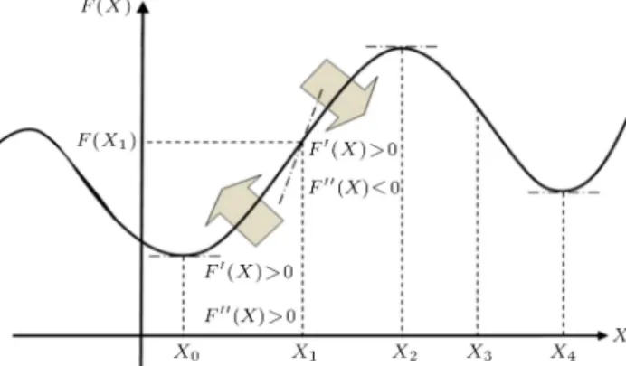
Figure 3 shows the local maximum, minimum, and inection points of the typical fth-degree polyno-mial angular curve. In this gure, if X0 is assumed to
be the start time of the fault, the portion between X0
and X4is considered as a stable rotor angle rst swing,
and F (X2) is the maximum value of angular position.
In this piece, a point such as X1 will denitely exist in
which the sign of curve concavity changes from positive to negative. SDM highlights the role of this point in improving the eciency of angular stability prediction. The local maximum, minimum, and inection points of the fth-degree polynomial are the roots of the rst- and second-order derivatives that are given as follows:
d^(t)
dt =5A5t4+4A4t3+3A3t2+2A2t+A1=0; (28)
d2^(t)
dt2 = 20A5t3+ 12A4t2+ 6A3t + 2A2= 0; (29)
where X0, X2, and X4 as the local minimum and
maximum points of the fth-degree polynomial curve are obtained through Eq. (28), and X1 and X3 as
inection points are the zeros of Eq. (29).
It should be noted that the aforementioned equa-tions are expressed in the continuous space, while
Figure 3. The local maximum, minimum, and inection points of the fth-degree polynomial curve.
PMUs measure and report data based on their tech-nical specications in the discrete space. Accordingly, the rst- and second-order derivatives in the discrete space are derived as follows:
((t)) t =
(t) (t t)
t ;
((t t))
t =
(t t) (t 2t)
t ; (30)
2((t))
t2 =
(t) (t t)
t (t t) (t 2t)t
t
=(t) 2(t t) + (t 2t)(t)2 ; (31)
where t is the time dierence between two successive PMU reported data. By considering Eqs. (30) and (31), calculating the rst- and second-order derivatives re-quires one and two PMU reporting time elapsed, respectively. In other words, the calculation of the second-order derivative in each time step is based on two time steps ago. These calculations are also valid for the rst swing of the fth-degree polynomial.
4. Prediction of power system angular stability based on SDM
The rotor angle of the generating unit is the main data for the transient stability prediction. Rotor angle can be computed by solving the swing equation and the electrical output power of generator [6,26]. The shortcomings of such techniques include determination of the initial value of rotor angle, lack of online access to the inertia constants, and variations in inertia constant by physical and geometrical structural changes [26,29]. The generator rotor angle and the associated terminal bus phase angle have the same variation trend. Even though they are not exactly equal, in some transient stability prediction methods, the generator rotor angle is hence estimated with voltage phase angle at PCC of power plant transformer to the bulk power grid [8]. In this paper, this assumption is taken into account. Bus phase angle is measured by PMU synchronized with the high-accuracy Global Positioning System (GPS). In terms of sampling and reporting rates of PMUs, the DW required for predicting angular stability is specied.
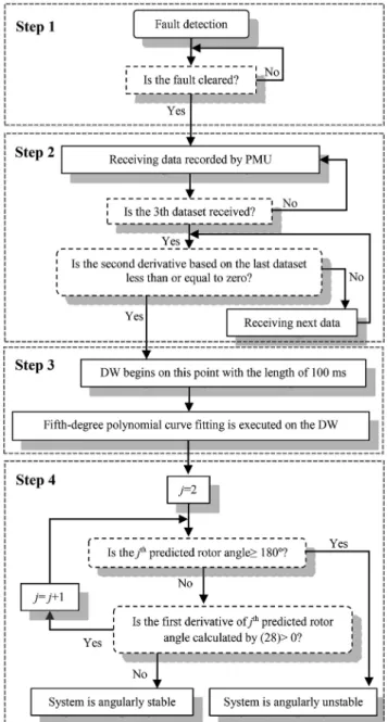
Figure 4 depicts the general scheme of the SDM for predicting the angular stability of the power system. The algorithm consists of four main steps explained in the following:
Step 1: Transient stability prediction methods are stimulated if a fault is detected on the power system. On this basis, the rst step of the SDM consists of
Figure 4. Flowchart of SDM for the prediction of power system angular stability.
fault detection in the transmission system and fault clearing time. These requirements can be fullled based on PMU data [30]. At the fault clearing time, the next step begins;
Step 2: Following the fault clearance, the voltage phase angle at the PCC of power plant transform-ers to the bulk power grid, which is continuously measured by PMU, is loaded in the SDM algorithm. This process continues until the third data becomes available. Accordingly, Eq. (31) is calculated for all subsequent data. When the second-derivative becomes zero or negative, the calculation stops. At this data point, the curve concavity changes from positive to negative. The third step will start at this point;
Step 3: Based on the result of Step 2, the calculation of the DW starts to ll up with PMU data. The length of the DW is in terms of the PMU reporting rate. According to IEEE Standard for Synchrophasor Measurements (IEEE std C37.118) [31], PMU shall support various data reporting rates associated with the nominal frequency of power systems. For 50 Hz system, supported rates are 10, 25, 50 Hz while a reporting rate of 100 Hz is permissible, too. Without loss of generality, a 100 ms DW is adopted here. This DW consists of 10 post-fault samples measured by PMU. When the DW is lled out, the fth-degree polynomial curve tting is estimated. The obtained curve is used as an input data for the nal step of processing;
Step 4: In the nal step, there are two comple-mentary parts that ultimately predict the angular stability of the power network. In the rst part, the rst-order derivative of the resultant curve known as the curve slope is calculated by Eq. (28). This part starts with the second predicted dataset. In the next part, the slope sign is to be determined at each data point. This process is applied only to the predicted rotor angle value less than or equal to 180 degrees. The boundary rotor angle is 180 degrees; the system is unstable if the predicted value exceeds this threshold. For the predicted rotor angle less than 180 degrees, two scenarios are expected as follows:
Unstable cases: If the slope sign is always positive, it becomes clear that the rotor angle is constantly growing and denitely passes the boundary value (Cases 2 and 3 in Figure 1);
Stable cases: Positive and negative signs reect
the growth and, then, the decline of the predicted curve. Rotor angle grows after the fault clearance; however, its growth stops before crossing the sta-bility boundary. As a result, the system stasta-bility is maintained at the rst swing (Cases 1 and 4 in Figure 1).
5. Numerical study
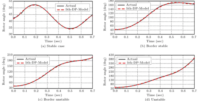
This section examines the proposed scheme for a practical SIME, as shown in Figure 2. This system incorporates a generating unit rated at 128 MVA and 115 MW with an inertia constant of 3.18 seconds, which is connected to the 400-kV substation through one 12.7/400 kV transformer. A PMU device is installed on the high-voltage side of the substation. The sampling and reporting rates of the PMU are 10 kHz and 100 sample/s, respectively. The subsystem is connected to the external grid as the innite bus through two high-voltage transmission lines. To perform simulation, the DIgSILENT software package [32] is used. Data analy-sis process is performed in the MATLAB environment. The three-phase fault (LLL) is supposed to be located at 0.1% of L2, which occurs at t = 0. The CCT is 0.329 sec. Therefore, the fault is cleared by opening the line circuit breaker after t = 0:07, 0.328, 0.330, and 0.35 to simulate the stable, border stable, border unstable, and unstable cases, respectively. The simulation results in the case of SIME are depicted in Figure 5. Here, the model (5th order) is able to accurately follow the rotor angle trajectory in all cases, and the validity of the model is proven, especially for the rst swing. For the purpose of validation, the simulations of dierent fault locations, fault duration, and loading levels are
performed. The results show that the 5th-order model enjoys satisfactory accuracy and the closest value with respect to the actual rotor angle trajectory. Moreover, this model is selected to be used in the rotor angle stability prediction process.
The proposed methodology predicts the transient instability status based on the local data, and the characteristics of the system will have no eect on the process and its implementation. Therefore, this approach and the SIME are examined on the WSCC nine-bus test system, as depicted in Figure 6. G1 is a salient pole generator and believed to be the reference generator at WSCC test bed. G2 and G3 are of the round rotor types and operate in the PV mode. The excitation system of all generators is IEEE DC1 and represented by a full-order model. The conditions stimulating the angular stability cases are as follows:
Fault type, duration, and location: Symmetrical and asymmetrical faults with two dierent durations, 120 ms and 100 ms, are simulated at various loca-tions on lines 7-8 and 7-5. The fault resistance is assumed to be 0.8 ;
Pre-fault system operation status: The generation level of power plant G2 changes, while the system conguration is kept unchanged. This level de-creases until the generating unit becomes stable even in 120 ms three phases to ground (LLLG) fault at the beginning of each line. Keeping the system load unchanged, generator G1 as the referenced generator compensates the reduced generation;
Special cases: In a real power network, when an asymmetrical fault occurs in a three-phase line, the associated circuit breaker in each phase clears fault independently of the other phases. Although the system angular stability behavior will change after opening each phase, the fault clearing time should
Figure 6. Single-line diagram of WSCC 9-bus test system.
be specied based on the time of the last opened phase.
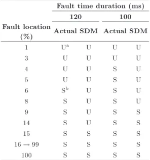
Table 1 presents the obtained results in terms of 100 ms and 120 ms LLLG faults located at various locations along line 7-5. The generation level of G2 as a pre-fault system operation status is kept equal to 145 MW. In this table, S and U denote stable and unstable predictions, respectively, and the actual column is determined based on numerical stability assessment methods. Results in Column 2 or 4 in Table 1 demonstrate that the system is angularly unstable at the fault location near bus 2 (power plant bus). According to Equal Area Criterion (EAC), it can be proven that, for the fault closer to the bus, the eective impedance between fault and power plant bus is reduced and the acceleration area increases. In such a stressed situation, the system is more likely to remain unstable. The comparison of fault time durations shows that the longer fault duration (more stressed situation) raises the probability of system instability for a fault at the same location. This conclusion can also be proven based on EAC. The results of Table 1 show the correctness of SDM prediction in an unstable situation. However, in the fairly stressed conditions in which the power system maintains its stability, the probability of wrong prediction is high.
The time required to carry out all SDM processing steps and predict the angular stability, after the com-pletion of the DW, is less than only 1 ms. The reason is that SDM predicts the stability status of the power sys-tem based on two simple Eqs. (30) and (31). The sim-plicity, low computational burden, and very short
pro-Table 1. Angular stability prediction results for PG2 = 145 MW and LLLG fault types along line 7-5.
Fault time duration (ms)
120 100
Fault location
(%) Actual SDM Actual SDM
1 Ua U U U
3 U U U U
4 U U S U
5 U U S U
6 Sb U S U
8 S U S U
9 S U S S
14 S U S S
15 S S S S
16 ! 99 S S S S
100 S S S S
cessing time are the unprecedented features of the real-world implementation of the proposed methodology.
In order to evaluate the performance of the proposed method, SDM is compared with the curve tting-based (CF) rotor angle trajectory method with a xed DW. For all simulation studies, both of the aforementioned methods use 100 ms calculation DW after clearing the fault for predicting the angular stability. The dierence between these two methods is the start point of the DW. SDM exploits a moving start point; however, CF uses a xed start point, which is the rst data right after the fault clearance.
To see the fault location eect on the accuracy of both prediction methods, the LLLG fault as a severe one is applied for 120 ms to 3% and 20% of line 5-7 at the G2 generation level equal to 145 MW. In Figure 7, the fault is examined on the 3% of line 5-7. Since the fault location is too close to bus 2, it inicts greater angular stability eect on the system. In addition to the actual phase angle of the power system as a benchmark curve obtained by the time domain simu-lation, the resultant curves of CF and SDM prediction processes are depicted. According to the actual curve, the system becomes unstable after the fault clearance since the bus phase angle is constantly growing with a positive slope and, nally, passes the boundary value (180). According to Figure 7, both CF and SDM can
correctly predict the system's angular instability after clearing the fault. However, the SDM resultant curve is closer to the actual phase angle in bus 2.
In another simulation, the fault is applied on 20% of line 5-7. The actual bus angle, CF, and SDM predicted curves are shown in Figure 8. According to this gure, the actual bus phase angle value returns back after clearing the fault and the system is stable within the rst swing duration. As can be seen in Figure 8, CF predicted curve is continuously increasing, showing instability. However, SDM, which uses a moving DW, returns back and predicts a stable case correctly.
Figure 7. Actual, CF, and SDM angular stability curves associated with an LLLG fault on 3% of line 5-7, PG2 = 145 MW.
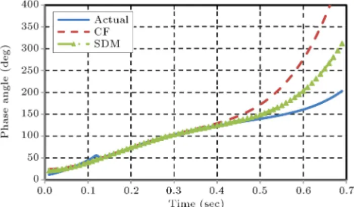
In Figure 9, the actual, CF, and SDM phase angle curves for the 120 ms LG fault located on 0% of line 7-5 at PG2 = 150 MW are shown. This gure represents that the SDM predicted curve is more accurate than the CF one in terms of following the actual path of the rotor angle. However, both of them predict the stability of the power system correctly.
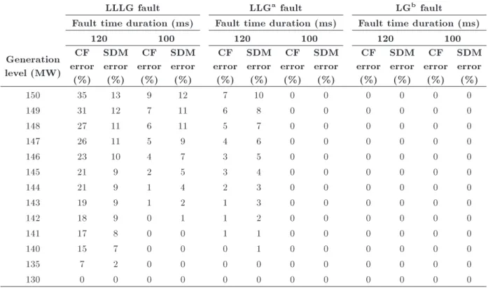
SDM as a response-based approach does not require equipment models and system conguration and operation status. However, the performance of the response-based angular stability prediction method depends on not only the fault location, but also the power plant generation level, fault duration, and fault type. Table 2 shows the results associated with various generation levels of G2 such as pre-fault system operation status, fault duration, fault type, and fault location on line 7-5. Columns 2 to 5, 6 to 9, and 10 to 13 of Table 2 show the prediction error of each method in stable/unstabe situations for LLLG, LLG, and LG fault types, respectively. The prediction error percentage of both CF and SDM is obtained through the following steps: 1) selecting fault type and duration, 2) choosing generation levels of power plant G2, and 3) locating fault on every percent of each
Figure 8. Actual, CF, and SDM angular stability curves associated with an LLLG fault on 20% of line 5-7, PG2 = 145 MW.
Figure 9. Actual, CF, and SDM angular stability curves associated with an LG fault on 0% of line 5-7, PG2 = 150 MW.
Table 2. Prediction error of CF and SDM methods in various simulation scenarios when the fault is on line 7-5.
LLLG fault LLGa fault LGb fault
Fault time duration (ms) Fault time duration (ms) Fault time duration (ms)
120 100 120 100 120 100
Generation level (MW)
CF error
(%)
SDM error (%)
CF error
(%)
SDM error (%)
CF error
(%)
SDM error (%)
CF error
(%)
SDM error (%)
CF error
(%)
SDM error (%)
CF error
(%)
SDM error (%)
150 35 13 9 12 7 10 0 0 0 0 0 0
149 31 12 7 11 6 8 0 0 0 0 0 0
148 27 11 6 11 5 7 0 0 0 0 0 0
147 26 11 5 9 4 6 0 0 0 0 0 0
146 23 10 4 7 3 5 0 0 0 0 0 0
145 21 9 2 5 3 4 0 0 0 0 0 0
144 21 9 1 4 2 3 0 0 0 0 0 0
143 19 9 1 2 1 3 0 0 0 0 0 0
142 18 9 0 1 1 2 0 0 0 0 0 0
141 17 8 0 0 1 1 0 0 0 0 0 0
140 15 7 0 0 0 1 0 0 0 0 0 0
135 7 2 0 0 0 0 0 0 0 0 0 0
130 0 0 0 0 0 0 0 0 0 0 0 0
aLLG: Two phases to ground;bLG: Single phase to ground.
line length; in addition, eventually, 4) in each step of these simulations, if the actual and predicted curves show the opposite system stability status, prediction error increases by 1%. This process is carried out for all fault types and durations, generation levels, and fault locations along lines 7-5 and 7-8. In the most stressed situation (LLLG fault, high generation level, and 120 ms fault duration), results show that SDM outperforms CF method. In other words, angular stability prediction results have improved by 5% in the worst situation for PG2 = 135 MW and by 22% at PG2 = 150 MW generation level in the best situation.
In order to further investigate the performance of the two aforementioned methods, special cases consist-ing of LLLG, LLG, and LG faults located on 0% of lines 7-5 and 7-8 at PG2 = 150 MW are simulated. In these studies, faulty or healthy phases open at dierent times and CCT is considered as the opening time of the last phase. For example, consider an LLLG fault where phases A, B, and C open after 110, 115, and 120 ms, respectively. In this case, CCT is 120 ms. In these cases, SDM and CF can correctly predict the stability/instability of the angular behavior of the power system.
As mentioned in Table 2, in addition to the same performance of SDM and CF in many case studies, in some situations, SDM is more accurate than CF for predicting angular stability and, in other cases, vice versa. However, in order to make a comprehensively
sound judgment on SDM performance and a complete comparison between performances of these two angular stability prediction methods, two quantitative and one qualitative comparisons are conducted in the following:
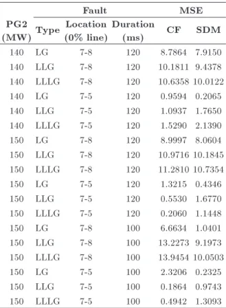
MSE comparison: This study gives numerical indices that determine the mismatch between pre-dicted and actual responses [29]. In order to make quantitative comparisons between SDM and CF in predicting the generating unit's rotor angle values, the Mean Squared Errors (MSE) of the actual and predicted responses are calculated as follows:
MSE =DS1 rXDS
p=1(C ^OAp COAp)2: (32)
where p is the index for the sample associated with the predicted and actual responses, respectively, DS is the number of all data points, C ^OAp and COAp
and are the Center Of inertia Angle (COA) associ-ated with the predicted and actual responses. COA as an important index in power system transient stability studies is formulated as follows:
COA =
NGP
g=1(Hg g) NGP g=1Hg
; (33)
where H is the inertia constant and NG is the total number of generators in the power system.
Table 3. Comparison of MSE of CF and SDM.
Fault MSE
PG2
(MW)Type Location(0% line)
Duration
(ms) CF SDM
140 LG 7-8 120 8.7864 7.9150
140 LLG 7-8 120 10.1811 9.4378 140 LLLG 7-8 120 10.6358 10.0122
140 LG 7-5 120 0.9594 0.2065
140 LLG 7-5 120 1.0937 1.7650 140 LLLG 7-5 120 1.5290 2.1390
150 LG 7-8 120 8.9997 8.0604
150 LLG 7-8 120 10.9716 10.1845 150 LLLG 7-8 120 11.2810 10.7354
150 LG 7-5 120 1.3215 0.4346
150 LLG 7-5 120 0.5530 1.6770 150 LLLG 7-5 120 0.2060 1.1448
150 LG 7-8 100 6.6634 1.0401
150 LLG 7-8 100 13.2273 9.1973 150 LLLG 7-8 100 13.9454 10.0503
150 LG 7-5 100 2.3206 0.2325
150 LLG 7-5 100 0.1864 0.9743 150 LLLG 7-5 100 0.4942 1.3093
MSE as a quantitative index is calculated for 18 dierent case studies and given in Table 3. Ac-cording to these results, at a time duration equal to 300 ms after the DW is lled out, the nal predicted curves obtained by SDM have a performance closer to the actual measurements, although, in rare cases, the response of the CF has a lower MSE index.
Generally, it can be concluded that the rotor angles predicted by SDM are of higher accuracy.
Probabilistic comparison: The wrong prediction of the system's angular behavior based on SDM and CF is presented in Table 2. These results can be used to calculate the generation level-based wrong prediction probability index, the type, time, and locations of the faults. The generation level-based wrong prediction probability is:
Pgb=
X2 l=1
3
X
e=1
Pl(We\ Ee)
!
; (34)
where P (W \ E) is the probability that wrong prediction (W ) and fault (E) occur together. The lines (1, 2) and fault types (LG, LLG, and LLLG) are denoted by l and e, respectively. According to probability rules, P (W [ E) can be expanded as follows:
P (We\ Ee) = P (WejEe) P (Ee); (35)
Figure 10. Generation level-based wrong prediction probability of CF and SDM.
where P (WejEe) is the probability of wrong
predic-tion in case of event Ee occurrence and is shown
in Tables 2 and 3. In [33], the P (Ee) is dened
as 80%, 15%, and 5% for LG, LLG, and LLLG fault types, respectively. By using these values and applying Eqs. (34) and (35), the generation level-based wrong prediction probability is achieved. In Figure 10, Pgbof CF and SDM is demonstrated. The
results show that, in simulated scenarios, SDM's performance is better than CF's. In addition, results of Figure 10 reveal the greater accuracy of the proposed angular stability prediction approach, compared to CF method.
Qualitative comparison: This comparison is made with an assumption that both of the predicted and actual behaviors of the system have similar trajectories; in other words, they feature stable or unstable angular curves. The interesting piece of results is that both methods can predict unstable situations correctly and there is no error when the power system is more stressed. In accordance with the power system protection principles, in angular unstable situations, the proper function of SPS is stimulated based on which the output of these meth-ods is guaranteed. Therefore, the dependability of protective equipment will be perfect. Dependability means the certainty that the SPS operates when its function is required. In all circumstances such as angular instability, which may cause the system collapse, this performance is required [23].
The other aspect of the protection system is security. Security is the certainty that the SPS will not operate when its function is not required. Ac-cording to the obtained result, although security is not quite satisfactory, it is acceptable. Dependability and security together suggest that protection in terms of system stability will operate properly. With respect to the qualitative considerations, the prediction schemes of SDM and CF are conrmed.
6. Conclusions
A response-based approach using PMU measurement data, polynomial rotor angle trajectory model, and SDM was proposed in this paper for the angular stability prediction of power system. The performance of the new method was testied on the WSCC 9 bus test bed. Based on a comprehensive suite of simulations, the actual responses of the proposed method were compared with the results of the existing angular stability prediction method based on curve tting. It was demonstrated that the proposed method had signicant characteristics including requiring only bus voltage phase angle, very low computation bur-den and prediction time, indepenbur-dence of equipment models and system conguration and operation status, simplicity in application, and better generation level-based wrong prediction probability. Considering these features, the utilization of this method in SPS and GRS could be promising, although more improvements in the security of the method are still requested. Further-more, according to the new fast communication media such as optic ber, it is proposed to investigate the feasibility of using SDM in Wide-Area Measurement, Protection, and Control System (WAMPAC).
Nomenclature
CN Parameter vector
Ck Polynomial coecients
COA Center Of inertia Angle D Damping factor (MW/Hz) DS Number of all data points FN Equation matrix
g Index of generators H Inertia constant
i Index of future time instants j Index of sample points
k Index of polynomial coecients l Index of line
m Index of future sample points MSE Mean Squared Errors
n Rotor angle polynomial order NG Total number of generators NS Number of samples in DW O(N) Observation vector
p Index of predicted and actual samples Pa Accelerating power (p.u.)
Pe Output electrical power (p.u.)
Pm Input mechanical power (p.u.)
t Time (sec)
T(N) Time matrix
wd Angular velocity of machine small-signal swings (Rad/sec)
W0 Nominal synchronous speed (Rad/sec)
j Measured rotor angle value (Rad)
^j Predicted rotor angle value (Rad)
t Time duration between two consecutive
samples (ms)
Initial rotor angle (Rad)
References
1. Khandani, A. and Akbari Foroud, A. \Providing tran-sient stability by excitation system response improve-ment methods through long-term contracts", Scientia Iranica, 26(3), pp. 1652-1663 (2019).
2. Aminifar, F., Fotuhi-Firuzabad, M., Safdarian, A., et al. \Synchrophasor measurement technology in power systems: panorama and state-of-the-art", IEEE Ac-cess, 2, pp. 1607-1628 (2014).
3. Kundur, P., Power System Stability & Control, Tata McGraw-Hill, Ed., 5th Reprint, New Delhi (2008).
4. Chih-Wen, L., Mu-chun, S., Shuenn-Shing, T., et al. \Application of a novel fuzzy neural network to real-time transient stability swings prediction based on syn-chronized phasor measurements", IEEE Transactions on Power Systems, 14, pp. 685-692 (1999).
5. Xiaochen, W., Jinquan, Z., Aidong, X., et al. \Review on transient stability prediction methods based on real time wide-area phasor measurements", 4th Int. Conf. on Electric Utility Deregulation and Restructuring and Power Technologies., pp. 320-326 (2011).
6. Karady, G.G. and Jun, G. \A hybrid method for generator tripping", IEEE Transactions on Power Systems, 17, pp. 1102-1107 (2002).
7. Hazra, J., Reddi, R.K., Das, K., et al. \Power grid transient stability prediction using wide area syn-chrophasor measurements", 3rd IEEE PES Innovative Smart Grid Technologies Europe (ISGT Europe), pp. 1-8 (2012).
8. Esmaili, M., Hajnoroozi, A.A., and Shayanfar, H.A. \Risk evaluation of online special protection systems", International Journal of Electrical Power & Energy Systems, 41, pp. 137-144 (2012).
9. Kun, M., Xu, P., Zhao, J., et al. \Comparison of methods for the perturbed trajectory prediction based on wide area measurements", IEEE Power Engineering and Automation Conference (PEAM), pp. 321-325 (2011).
10. Liu, C.W. and Thorp, J. \Application of synchronised phasor measurements to real-time transient stability prediction", IEE Proceedings - Generation, Transmis-sion and Distribution, 142, pp. 355-360 (1995).
11. Hashiesh, F., Mostafa, H.E., Khatib, A.R., et al. \An Intelligent wide area synchrophasor based system for predicting and mitigating transient instabilities", IEEE Transactions on Smart Grid, 3, pp. 645-652 (2012).
12. Siddiqui, S.A., Verma, K., Niazi, K.R., et al. \Real-time monitoring of post-fault scenario for determining generator coherency and transient stability through ANN", IEEE Transactions on Industry Applications, 54(1), pp. 685-692 (2018).
13. Zhou, Y., Wu, J., Hao, L., et al. \Transient stability prediction of power systems using post-disturbance rotor angle trajectory cluster features", Electric Power Components and Systems, 44(17), pp. 1879-1891 (2016).
14. Tingyan, G. and Milanovi, J.V. \The eect of quality and availability of measurement signals on accuracy of on-line prediction of transient stability using decision tree method", IEEE PES ISGT Europe, pp. 1-5 (2013).
15. Guo, T. and Milanovi, J.V. \On-line prediction of tran-sient stability using decision tree method; sensitivity of accuracy of prediction to dierent uncertainties", IEEE Conf. PowerTech. Grenoble, pp. 1-6 (2013).
16. Sun, K., Lee, S.T., and Zhang, P. \An adaptive power system equivalent for real-time estimation of stability margin using -plane trajectories", IEEE Transactions on Power Systems, 26, pp. 915-923 (2011).
17. Bretas, N.G. and Phadke, A.G. \ Real time instability prediction through adaptive time series coecients", IEEE Power Engineering Society, Winter Meeting, pp. 731-736 (1999).
18. Alinezhad, B. and Karegar, H.K. \Predictive out-of-step relay based on equal area criterion and PMU data", Int Trans Electr Energ Syst, 27:e2327 (2017).
19. Zare, H., Alinejad, B.Y., and Yaghobi, H. \Intelligent prediction of out-of-step condition on synchronous generators because of transient instability crisis", Int Trans Electr Energ Syst., 29:e2686 (2019).
20. Sobbouhi, A.R. and Aghamohammadi, M.R. \A new algorithm for predicting out-of-step using rotor speed-acceleration based on phasor measurement units (PMU) Data", Electric Power Components and Sys-tems, 43, pp. 1478-1486 (2015).
21. Diaz-Alzate, A.F., Candelo-Becerra, J., and Villa Sierra, J. \Transient stability prediction for real-time operation by monitoring the relative angle with predened thresholds", Energies MDPI, Open Access Journal, EE 423, 12(5), pp. 1-17 (March 2019).
22. Bhui, P. and Senroy, N. \Real-time prediction and control of transient stability using transient energy function", IEEE Transactions on Power Systems, 32(2), pp. 923-934 (2017).
23. Zima, M. \Special protection schemes in electric power systems", EEH-Power Systems Laboratory, pp. 1-22 (2002).
24. Guo, H., Liu, C.C., and Wang, G. \Lyapunov expo-nents over variable window sizes for prediction of rotor angle stability", North American Power Symposium, pp. 1-6 (2014).
25. Weihui, F., Sanyi, Z., McCalley, J.D., et al. \Risk as-sessment for special protection system", IEEE Trans-actions on Power Systems, 17, pp. 63-72 (2002).
26. Rahimi Pordanjani, I., Askarian Abyaneh, H., Sadeghi, S.H.H., et al. \Risk reduction in special protection systems by using an online method for transient insta-bility prediction", International Journal of Electrical Power & Energy Systems, 32, pp. 156-162 (2010).
27. Weckesser, T., Johannsson, H., and stergaard, J. \Impact of model detail of synchronous machines on real-time transient stability assessment", IREP Symposium Bulk Power System Dynamics and Control -IX Optimization, Security and Control of the Emerging Power Grid, Rethymno, pp. 1-9 (2013).
28. Teimourzadeh, S., Davarpanah, M., Aminifar, F., et al. \An adaptive auto-reclosing scheme to preserve transient stability of microgrids", IEEE Transactions on Smart Grid, 9(4), pp. 2638-2646 (2016).
29. Hajnoroozi, A.A., Aminifar, F., and Ayoubzadeh, H. \Generating unit model validation and calibration through synchrophasor measurements", IEEE Trans-actions on Smart Grid, 6, pp. 441-449 (2015).
30. Gopakumar, P., Reddy, M.J.B., and Mohanta, D.K. \Transmission line fault detection and localisation methodology using PMU measurements", IET Gener-ation, Transmission & Distribution, 9, pp. 1033-1042 (2015).
31. IEEE standard for synchrophasor measurements for power systems. IEEE Std C37.118.1-2011 (Revision of IEEE Std C37.118-2005), pp. 1-61 (2011).
32. DIgSILENT PowerFactory, available at:/http://www. digsilent.de/.
33. Lucas, J.R. \Power system analysis: faults", EE 423 (2005).
Biographies
Ali A. Hajnoroozi was born in Golpayegan, Iran in 1987. He received the BSc degree from the Isfahan Uni-versity of Technology, Isfahan, Iran in 2009 and, then, obtained the MSc (Hons.) degree from the Iran Univer-sity of Science and Technology, Tehran, Iran in 2011, both in Electrical Engineering. He is currently with Iran University of Science and Technology, Tehran, Iran, as a PhD student. His current research interests include wide-area measurement systems, transient and voltage stability, special protection schemes, and model validation.
Heidar Ali Shayanfar received the BS and MSE degrees in Electrical Engineering in 1973 and 1979,
respectively, and obtained the PhD degree in Electrical Engineering from Michigan State University, Lansing, MI, USA in 1981. He is currently a Full Professor at the Department of Electrical Engineering, Iran University
of Science and Technology, Tehran, Iran. His current research focuses on the application of articial intelli-gence to power system, dynamic load modeling, voltage collapse, and smart grid.