Efficiency distribution and expected efficiencies in DEA with imprecise data

(1)

185

Efficiency distribution and expected efficiencies in DEA with

imprecise data

Bohlool Ebrahimi

1* 1

Satellite Research Institute, Iranian Space Research Center, Tehran, Iran

[email protected]

Abstract

Several methods have been proposed for ranking the decision making units (DMUs) in data envelopment analysis (DEA) with imprecise data. Some methods have only used the upper bound efficiencies to rank DMUs. However, some other methods have considered the both of the lower and upper bound efficiencies to rank DMUs. The current paper shows that these methods did not consider the DEA axioms and may be unable to produce a rational ranking. We show that considering the imprecise data as stochastic and using the expected efficiencies to rank DMUs give better results. Indeed, we propose a new ranking approach, based on considering the DEA axioms for imprecise data that removes the existing drawbacks. Some numerical examples are provided to explain the content of the paper.

Keywords: Data envelopment analysis (DEA), efficiency measure, expected efficiencies, imprecise data

1-Introduction

Charnes et al. (1978) developed data envelopment analysis (DEA) for performance evaluation of several similar decision making units (DMUs). In this model, it is supposed that the values of inputs and outputs are exactly known. However, in many real applications, these values are imprecise.

Imprecise data have various types: interval (bounded) data, weak and strong ordinal data, ratio bound data, multiplied order data, and so on. The mathematical representation of these data is given in Park (2007). So far, different approaches have been developed to calculate the relative efficiencies with the imprecise data in DEA. Some methods are given to rank DMUs based on only the upper bound efficiencies (Cooper et al. 1999, 2001; Kim et al. 1999; Lee et al. 2002; Zhu 2003, 2004; Park 2004). Some other methods are developed to calculate the lower and upper bound efficiencies to rank DMUs (Despotis and Smirlis 2002; Wang et al. 2005; Kao 2006; Park 2007).

Cooper et al. (1999) considered the interval and weak ordinal data in DEA and named the new nonlinear model as imprecise DEA (IDEA). They converted the model into an equivalent linear model through the scale transformation and variable alterations. Kim et al. (1999) used IDEA for performance evaluation in Telephone offices. Lee et al. (2002) extended the IDEA concept to the additive DEA model. Despotis and Smirlis (2002) developed two linear programming to estimate the lower and upper bound efficiencies by considering the pessimistic and optimistic state for each DMU.

*Corresponding author

Vol. 12, No. 1, pp. 185-197 Winter (January) 2019

(2)

186

Zhu (2003) showed that the scale transformation in the Cooper et al. (1999, 2001) approach is redundant. He converted the interval and weak ordinal data into the exact data to estimate the relative efficiencies.

Zhu (2004) used the method for performance evaluation in the Korean Mobile Telecommunication Company. Zhu (2003) and Park (2004) have used the same variable alteration to convert the nonlinear IDEA model into a linear model.

Wang et al. (2005) proposed two linear mathematical programming to obtain the lower bound and upper bound efficiencies by considering a unique production frontier for all DMUs. Kao (2006) emphasized that the efficiency scores should be imprecise in the presence of imprecise data. He proposed two two-level mathematical programming to calculate the lower bound and upper bound efficiencies. Park (2007) used the concept of supremum and infimum and proposed a mathematical programming for calculating the lower bound efficiencies.

Park (2010) investigated the dual model of IDEA and its relationships with primal problem based on the duality theory in IDEA. Marbini et al. (2014) investigated the performance evaluation in the presence of interval data, without sign restrictions. He et al. (2016) developed some DEA models to improve the inputs and outputs of inefficient DMUs such that their upper bound efficiency scores become one, in the presence of interval data. Ebrahimi et al. (2017) proposed a new nonlinear model to efficiency measure in the presence of both general weight restrictions and different types of imprecise data. They proposed a simulation-based genetic algorithm to estimate the efficiencies. Ebrahimi and Rahmani (2017) developed a mixed integer DEA model to find the best BCC-efficient DMUs by solving only one model. Ebrahimi and Khalili (2018) developed a new mixed integer DEA model to find the best DMU in the presence of both weight restrictions and different types of imprecise data. They utilized the model to find the best supplier in the presence of assurance region type I and interval and ordinal data. Ebrahimi et al. (2018) investigated the existing methods to estimate the efficiencies in the presence of interval and ordinal data. They illustrated some drawbacks of the existing methods and proposed a new method to calculate the efficiency scores.

It should be noted that the IDEA approach has been used to efficiency measure in many real-life applications. Farzipoor Saen (2007) applied the proposed method by Zhu (2003) for ranking the suppliers in the supplier selection problem. Asosheh et al. (2010) presented a mixed integer IDEA model to find the most efficient information technology (IT) projects. Ebrahimi et al. (2014) studied the drawbacks of the proposed model by Asosheh et al. (2010). They showed that the model is unable to find the best IT project and proposed a new approach to eliminate the drawbacks. Toloo and Nalchigar (2011) developed a new mixed integer imprecise DEA model to find the best supplier in the supplier selection problem. They used the proposed method of Zhu (2003) to handle the imprecise data and utilized their model to find the best supplier among 18 supplier in the presence of both interval and ordinal data.

Karsak and Dursun (2014) presented a supplier selection methodology by using the IDEA and Quality function deployment (QFD). Toloo (2014) presented a mixed integer programming IDEA model to determine the best supplier in the supplier selection problem. Chen et al. (2017) developed some mathematical DEA models to cope with bounded and Likert scale data. They have used the models for performance evaluation of the regional energy efficiency in China. Khalili-Damghani et al. (2015) applied the DEA model to efficiency measure of combined cycle power plant in the presence of interval data. Baghery et al. (2016) applied the DEA model to prioritize failures in the automotive industry with interval data. Toloo et al. (2018) developed some new DEA models to calculate the lower and upper bound efficiencies in the presence of interval dual-role factors. They used the models to efficiency measure in bank branches.

As literature review shows, different approaches have been developed to calculate the relative efficiency scores in the presence of imprecise data. In the next section, we show that considering the lower bound and upper bound efficiencies to rank DMUs may gives incorrect ranking. We explain the problems in the theory and use some numerical examples to clarify them. Therefore, the main contributions of the paper is as follows:

(3)

187

 Developing a new algorithm to rank DMUs, based on considering the DEA axioms for imprecise data. The algorithm eliminates the drawbacks.

It should be here emphasized that the proposed approach in this paper uses a set of exact data instead of imprecise data to calculates the efficiencies and expected efficiencies. To efficiency measure in the presence of random noise in terms of measurement errors, specification errors and also chance constraint DEA models the interested readers can refer to Olesen and Petersen (2016).

The rest of the paper is organized as follows: in section 2, we explain the drawbacks of the existing approaches. Section 3 explains the developed approach of this paper. Numerical examples and conclusions are given in sections 4 and 5, respectively.

2-The problems of the existing methods

This section explains the problems of the existing methods to efficiency measure in the DEA model with imprecise data. First, we study the proposed method by Park (2007). He applied the concept of supremum and infimum and developed the following model (1) to estimate the lower bound efficiency score of DMUp.

i r v u p j k j x x v y y u x x v y y u x x v t s y y u i r n i i i ij i m r r r rj r n i i i ip i m r r r rp r i i n i ip i r r m r rp r , , , , ,..., 1 , 0 } inf{ } sup{ 0 } sup{ } inf{ 1 } sup{ . . } inf{ max 1 1 1 1 1 1               



                   (1)

In this model i and



r

 represent the imprecise data for inputs and outputs, respectively.

It should be noted that the upper bound efficiency score can be calculated by using the mentioned methods in the previous section, such as Cooper et al. (1999, 2001) and Zhu (2003). The model to obtain the upper bound efficiency score is as follows:

1 1 1 1 max . . 1

0 , 1,..., ( )

( )

, 0 ,

m r rp r n i ip i m n

r rj i ij

r i

i ij i

r rj r

r i

u y s t

v x

u y v x j k

x x i

y y r

u v i r

                   



(4)

188

Based on the lower and upper bound efficiencies, Park (2007) classified DMUs into three groups, as follows.

Inefficient: the upper bound efficiency score is less than one.

Potentially efficient: the upper bound efficiency score is equal to unity, but the lower bound is less than

one.

Perfectly efficient: the lower bound efficiency score is equal to unity.

To solve the model (1), the procedure of calculating the Inf and Sup for ordinal data is as follows. Suppose the ith inputs of DMUs is in a weak ordinal format, as shown in (3).

ik p i ip p i i

i x x x x x

x₁ ₂... _, _₁  _, _₁... (3)

Since, DEA models have the unit-invariant property, therefore, Park (2007) normalized the data of relation (3) as shown in (4).

1 ...

...

0x_i'₁x_i'₂ x_i'_,_p_₁x_ip' x_i'_,_p_₁ x_ik'  (4) Now, the Inf and Sup are calculated as follows (DMUp is under evaluation):

p j x x x x x x x x x x x x x x ik p i ip p i i i ij ik p i ip p i i i ip                           , 0 } 1 ... ... 0 inf{ 1 } 1 ... ... 0 sup{ ' ' 1 , ' ' 1 , ' 2 ' 1 ' ' ' 1 , ' ' 1 , ' 2 ' 1 ' (5)

In other words, before solving the model (1), the weak ordinal data (3) is replaced with the following integer numbers.

p j x

x_ip1& _ij 0 

Obviously, these numbers are infeasible to use in the model (1). Indeed, the correct numbers are

1 0

&

1     

 b p x j p

x_ib _ij , to keep the relation (3).

To show the problem in more detail, let the numerical example is used in Park (2007). In this example, there are eight telephone offices with three inputs and three outputs. The data of third output is in the weak ordinal format as follows:

}

{ 34 35 33 37 31 36 32 38

8 3

3 x R x x x x x x x x

D         (6)

According to the Park (2007) approach, to evaluate the DMU1 the vector of x3*(1,0,0,0,0,0,0,0) is used instead of weak ordinal data (6), that is infeasible. However, applying the feasibility condition implies that we should use x₃*(1,0,1,1,1,0,1,0). Furthermore, Park (2007) method uses only zero and one for all ordinal data. It should be noted that, the probability of occurrence of these data is near to zero in practice.

The above discussion shows that Park (2007) has used a set of infeasible integer numbers instead of weak ordinal data. As a result, the obtained lower bound efficiency score will be incorrect with these data. It should be noted that Park (see the last paragraph on pp. 536) claimed that the efficiency score will be safe and sound if the exact data set is infeasible or not. But, it is so easy to give an example to show that the claim is incorrect.

Moreover, in the following example, we show that the Park (2007) method and also some other existing methods give incorrect result in some cases.

(5)

189

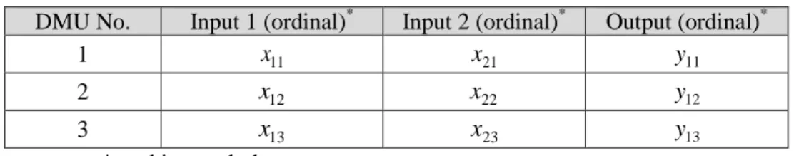
Example 1: Consider three DMUs, each uses two weak ordinal inputs to produce one ordinal output, as

given in table 1.

Table 1. Data for 3 DMUs

DMU No. Input 1 (ordinal)* Input 2 (ordinal)* Output (ordinal)*

1 x₁₁ x₂₁ y₁₁

2 x₁₂ x₂₂ y₁₂

3 x13 x23 y13

* ranking such that x13x12x11, x23x22x21, y11y12y13

It is easy to see that DMU3 dominates DMU2, and DMU2 dominates DMU1. In other words, a wise decision maker ranks these DMUs as: DMU3> DMU2> DMU1. However, we show that the existing methods give an incorrect ranking for the example.

Applying the proposed methods of Cooper et al. (1999, 2001), Zhu (2003, 2004), Park (2004) and other existing methods to calculate the upper bound efficiency scores, yield that all of the DMUs are efficient. It should be noted that just in one special situation, x₁₃x₁₂x₁₁ & x₂₃x₂₂x₂₁ & y₁₁y₁₂ y₁₃, that occurs with zero probability in practice, all of the DMUs are efficient.

Also, the existing methods to rank DMUs based on considering the both of lower and upper bound efficiencies give incorrect results. We use the approach of the Park (2007) to calculate the lower bound efficiencies. The efficiencies are calculated in both states, considering the feasibility condition and without considering the feasibility conditions. The results are summarized in table 2.

Table 2. The results of the Park (2007) method to calculate the lower bound efficiencies The DMU under

evaluation The values of variables

Without considering feasibility Considering feasibility

DMU1 DMU2 DMU3 DMU1 DMU2 DMU3

'* 11

x 1 0 0 1 1 1

'* 12

x 0 1 0 0 1 1

'* 13

x 0 0 1 0 0 1

'* 21

x 1 0 0 1 1 1

'* 22

x 0 1 0 0 1 1

'* 23

x 0 0 1 0 0 1

'* 11

y 0 1 1 0 0 0

'* 12

y 1 0 1 1 0 0

'* 13

y 1 1 0 1 1 0

Lower bound

efficiencies 0 0 0 0 0 0

The results show that based on Park (2007) approach, the efficiency scores of the three DMUs is equal to [0 , 1]. In other words, the DMUs have the same rank, that is unacceptable. It should be noted that the proposed methods by Despotis and Smirlis (2002), Wang et al. (2005) and Kao (2006) also gives a similar result. In other words, all of the existing methods produce incorrect ranking for the example.

(6)

190

In the next example, we find another problem in Park (2007) method. Indeed, we show that the method is unable to calculate the lower bound efficiencies in some cases.

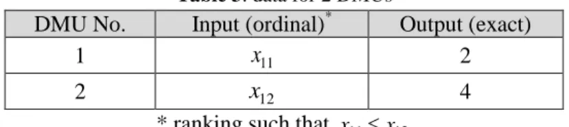
Example 2: Consider two DMUs, each uses one ordinal input to produce one precise output.

Table 3. data for 2 DMUs

DMU No. Input (ordinal)* Output (exact)

1 x11 2

2 x₁₂ 4

* ranking such that x11x12

The basic maximin DEA model to calculate the relative efficiency score is as follows:

     

   

     

   



 

i ij i r

rj r j

i ip i r

rp r r i v

u _v_x

y u Max x

v y u Max

i

r, 0, ,

(7)

The model can be converted to the linear CCR-DEA model (Khalili et al. 2010).

The result of calculating the Inf and Sup based on Park (2007) approach is presented in table 4. It is easy to see that it is impossible to calculate the efficiencies for these data by using the model (7), except DMU1 by considering the feasibility condition. So, the ranking of DMUs is not possible.

Table 4. The values of ordinal data by using the Park (2007) method

Overall, the drawbacks of the existing methods can be summarized as follows:

 Replacing ordinal data with a set of infeasible integer numbers to calculate the lower bound efficiencies. Obviously, the infeasible solutions lead to the incorrect optimal solution in the mathematical programmings.

 Produce incorrect ranking, as shown in the example 1.

 In some cases, the existing methods are unable to calculate the lower bound efficiencies, and so unable to rank DMUs.

 Using only zero and one instead of ordinal data that their occurrence possibility is near to zero in practice.

3-The proposed algorithm

The existing interval-data methods are capable to find the largest possible efficiency and the smallest possible efficiency scores. However, the probability of their occurrence is too small to have practical meaning. In the following, we propose a new method to rank DMUs in the presence of imprecise data, by considering the efficiency distribution. First, we mention the first axiom of the DEA that helps us to develop this method.

The DMU under evaluation The values of variables

Without considering feasibility Considering feasibility

DMU1 DMU2 DMU1 DMU2

'* 11

x 1 0 1 0

'* 12

x 0 1 1 1

Lower bound efficiencies Cannot be calculated

Cannot be

calculated 0.5

Cannot be calculated

(7)

191

The production possibility set (PPS) and the DEA model are based on some axioms. The first axiom is inclusion of observation. In the presence of imprecise data, there is not precise observed data to construct the PPS. To clarify the topic, consider the data presented in table 3. For this data, the PPS with constant returns to scale (CRS) technology is



(x,y)R2:x0&y4



that has been shown in figure 1. For this PPS, the production frontier is the line between (0,0) and (0,4), that is meaningless. In other words, by this PPS it is impossible to calculate the relative efficiencies. This problem shows that the DEA axioms are necessary to build the PPS and determine the production frontier. The previous methods did not consider the axiom that leads to the incorrect results.

To consider the inclusion of observation axiom, the imprecise data can be replaced with random numbers. In other words, we generate a sufficient amount of random data instead of imprecise data. More specially, for ordinal data of table 3, the random data can be generated as follows. First, we generate a random number in interval [0 , 1] for x12. Then, the value of x11 is randomly generated in interval of [0 , x12]. Since, there is no information about the probability distribution of the imprecise data, so it can be assumed uniform. In this case, the steps of the proposed algorithm are as follows:

 Generating uniform random data with N iterations.

 Calculating efficiencies for all DMUs with the data obtained from previous stage. At this stage, N efficiency scores for each DMU will be obtained.

 Calculating the average efficiency score of efficiencies. Indeed, the average efficiency is an estimation of the expected value of efficiencies.

 Ranking DMUs based on the expected efficiencies, DMUj1 dominates DMUj2 if and only if the expected efficiency score of DMUj1 is greater than DMUj2.

Obviously, increasing N leads to obtain the more exact expected efficiencies. If we were able to extract the efficiency distribution, we could calculate the exact value of expected efficiencies. Indeed, the average efficiency is an estimation of expected efficiency, so these values will be approximately equal by increasing the value of N. To show the benefits of the proposed approach we apply it to examples 1 and 2, in the next section.

4-Numerical illustration

In this section, to demonstrate the capability and applicability of the proposed method we apply it to the data presented in tables 1 and 3 and discuss the results.

Example 3: As discussed in example 1, the existing methods are unable to rank the three DMUs,

presented in table 1. We apply the proposed approach in the previous section for this example with 001

. 0





. The results are provided in table 5, for different values of N. The minimum, maximum, standard deviation (SD) and average efficiencies are calculated for each DMU. As we expected, the

DMU2

DMU1 PPS

y

x

Fig 1. PPS for the data presented in table 3

(8)

192

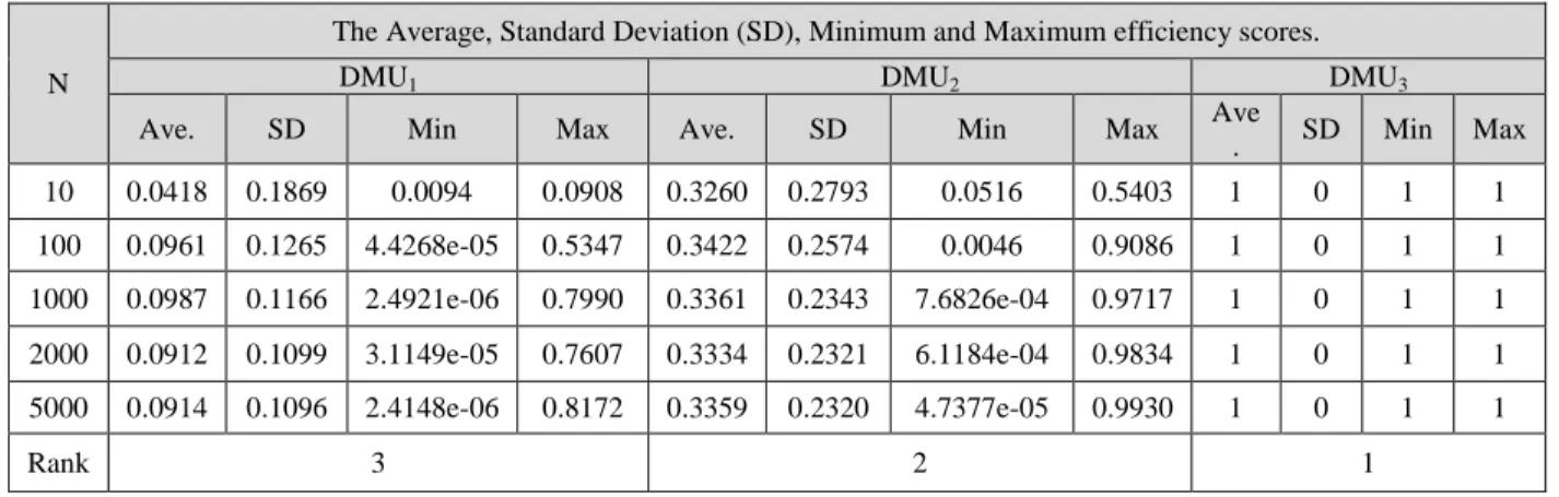
DMU3 is always efficient, for different values of N. But, the DMU1 and DMU2 are inefficient with the average efficiency scores of 0.0914 and 0.336, respectively. A visual inspection reveals that the averages efficiencies do not differ much for N1000_{for all DMUs. For}N2000 the differences between the average efficiencies appears at the third digit after the decimal point for all DMUs.

As it can be seen and also we expected, as the value of N increases, the lower bound and upper bound of the efficiencies expand accordingly.

Table 5. The result of the proposed approach for data presented in table 1

N

The Average, Standard Deviation (SD), Minimum and Maximum efficiency scores.

DMU1 DMU2 DMU3

Ave. SD Min Max Ave. SD Min Max Ave

. SD Min Max

10 0.0418 0.1869 0.0094 0.0908 0.3260 0.2793 0.0516 0.5403 1 0 1 1

100 0.0961 0.1265 4.4268e-05 0.5347 0.3422 0.2574 0.0046 0.9086 1 0 1 1

1000 0.0987 0.1166 2.4921e-06 0.7990 0.3361 0.2343 7.6826e-04 0.9717 1 0 1 1

2000 0.0912 0.1099 3.1149e-05 0.7607 0.3334 0.2321 6.1184e-04 0.9834 1 0 1 1

5000 0.0914 0.1096 2.4148e-06 0.8172 0.3359 0.2320 4.7377e-05 0.9930 1 0 1 1

Rank 3 2 1

It should be noted that considering the efficiency distribution is very important. In most of existing methods, only the lower and upper bound efficiencies are used to rank the DMUs. As it can be seen, for

5000



N , the average efficiency score of DMU2 is near to 0.336 with lower bound of 4.74*10 -5

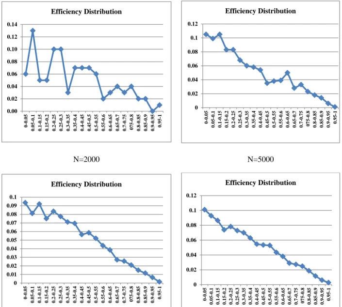
and upper bound of 0.993. The efficiency distribution of DMU2 is shown in figure 2 for different values of N. We divided the efficiency score of [0 , 1] into 20 equal segments. The Y-axis is the efficiency frequency for different range of efficiency. The charts show that the efficiency distribution is not uniform. If it was uniform, then the expected efficiency score of DMU2 was near to 0.5, instead of 0.336.

Also, we calculate the SD of efficiencies that shows the amount of variation or dispersion of efficiencies. A low SD implies that the data points tend to be close to the mean data, while a high SD implies that the data points are spread out over a wider range of values. As we expect, the SD of DMU3 is zero, since it’s lower bound efficiency score is equal to one, and so this DMU is perfectly efficient. Moreover, the SD of DMU2 is greater than the SD of DMU1. This is because the efficiency score of DMU2 varies between approximately zero and one but, the efficiency score of DMU1 varies between approximately zero and 0.81. It should be noted that by increasing the value of N the value of SD are reduced. This matter can be seen by considering the figure 2, that for large value of N the curve of efficiency distribution is more smooth.

(9)

193

N=100 N=1000

N=2000 N=5000

Fig 2. the efficiency distribution of DMU2 for different values of N

Example 4: in example 3, it is explained that the Park (2007) method is unable to calculate the efficiency

scores to rank the DMUs.

Now, we apply the proposed method for the example. The results summarized in table 6, show that the DMU1 with the expected efficiency of 0.844 has a better rank in comparing to DMU2 with the expected efficiency score of 0.757. Also, Since, the variation of efficiency scores of DMU1 is significantly less than the DMU2, so it’s SD is less than the SD of DMU2.

0.00 0.02 0.04 0.06 0.08 0.10 0.12 0.14 0-0. 0 5 0. 05-0. 1 0. 1-0 .15 0. 15-0. 2 0. 2-0 .25 0. 25-0. 3 0. 3-0 .35 0. 35-0. 4 0. 4-0 .45 0. 45-0. 5 0. 5-0 .55 0. 55-0. 6 0. 6-0 .65 0. 65-0. 7 0. 7-0 .75 075 -0. 8 0. 8-0 .85 0. 85-0. 9 0. 9-0 .95 0. 95-1 Efficiency Distribution 0 0.02 0.04 0.06 0.08 0.1 0.12 0-0. 0 5 0. 05-0. 1 0. 1-0 .15 0. 15-0. 2 0. 2-0 .25 0. 25-0. 3 0. 3-0 .35 0. 35-0. 4 0. 4-0 .45 0. 45-0. 5 0. 5-0 .55 0. 55-0. 6 0. 6-0 .65 0. 65-0. 7 0. 7-0 .75 075 -0. 8 0. 8-0 .85 0. 85-0. 9 0. 9-0 .95 0. 95-1 Efficiency Distribution 0 0.01 0.02 0.03 0.04 0.05 0.06 0.07 0.08 0.09 0.1 0-0. 0 5 0. 05-0. 1 0. 1-0 .15 0. 15-0. 2 0. 2-0 .25 0. 25-0. 3 0. 3-0 .35 0. 35-0. 4 0. 4-0 .45 0. 45-0. 5 0. 5-0 .55 0. 55-0. 6 0. 6-0 .65 0. 65-0. 7 0. 7-0 .75 075 -0. 8 0. 8-0 .85 0. 85-0. 9 0. 9-0 .95 0. 95-1 Efficiency Distribution 0 0.02 0.04 0.06 0.08 0.1 0.12 0-0. 0 5 0. 05-0. 1 0. 1-0 .15 0. 15-0. 2 0. 2-0 .25 0. 25-0. 3 0. 3-0 .35 0. 35-0. 4 0. 4-0 .45 0. 45-0. 5 0. 5-0 .55 0. 55-0. 6 0. 6-0 .65 0. 65-0. 7 0. 7-0 .75 075 -0. 8 0. 8-0 .85 0. 85-0. 9 0. 9-0 .95 0. 95-1 Efficiency Distribution

(10)

194

Table 6. The result of the proposed approach for data presented in table 3 N

The Average, Standard Deviation (SD), Minimum and Maximum efficiency scores.

DMU1 DMU2

Ave. SD Min Max Ave. SD Min Max

10 0.8923 0.1826 0.5263 1 0.5603 0.2742 0.0372 1

100 0.8687 0.1793 0.5014 1 0.7014 0.3003 0.0269 1

1000 0.8486 0.1810 0.5010 1 0.7511 0.3175 0.018 1

2000 0.8451 0.1846 0.5001 1 0.7579 0.3219 0.0019 1

5000 0.8443 0.1851 0.5000 1 0.7573 0.3244 7.1378e-05 1

Rank 1 2

This example shows that the efficiencies of average data differ from average efficiencies. Indeed, the expected values of x11 and x12 with the uniform data generation are 0.25 and 0.5, respectively. This average data implies that the two DMUs are both efficient. However, our proposed approach considers the expected efficiencies instead of the efficiencies of expected data. The efficiency distributions of DMU1 and DMU2 are shown in figure 3 and 4 for different values of N, respectively. The chart shows that more than 50% of efficiency frequency are in interval [0.95 , 1]. This matter implies that we need to consider the distribution of the efficiency scores in the interval. Most of existing methods rank DMUs based on just the lower and upper bound efficiencies, without considering the efficiency distribution.

Fig 3. The efficiency distribution of DMU1 for different values of N

0 0.1 0.2 0.3 0.4 0.5 0.6

(11)

195

Fig 4. the efficiency distribution of DMU2 for different values of N

5-Conclusions

The paper explains the drawbacks of the existing methods in the DEA to rank DMUs with imprecise data. We show that the methods did not consider the DEA axioms, so may produce incorrect ranking in some cases. It is shown that the Park (2007) method uses a set of infeasible integer data instead of imprecise data. It is also shown that in some cases, the method is unable to calculate the efficiencies or produces a rational ranking.

It was emphasized that the DEA model and the PPS are based on some axioms, especially the inclusion of observation axiom. It is shown that with imprecise data, we maybe unable to determine the PPS and the production frontier correctly. Therefore, by considering the DEA axioms, a simple practical algorithm is presented to rank DMUs in the presence of imprecise data.

The proposed approach considers the efficiency distribution and expected efficiencies to rank the DMUs, instead of the lower and upper bound efficiencies. It is explained that the approach covers the mentioned problems and gives more reliable results.

Acknowledgement

The author wish to thank the editor-in-chief and anonymous referees for their helpful comments.

0 0.1 0.2 0.3 0.4 0.5 0.6

(12)

196

References

Asosheh, A., Nalchigar, S., Jamporazmey, M. (2010). Information technology project evaluation: An integrated data envelopment analysis and balanced scorecard approach. Expert Systems With Applications, 37, 5931–5938.

Baghery, M., Yousefi, S., Jahangoshai Rezaee, M. (2016). Risk measurement and prioritization of auto parts manufacturing processes based on process failure analysis, interval data envelopment analysis and grey relational analysis. Journal of Intelligent Manufacturing, DOI: 10.1007/s10845-016-1214-1.

Charnes, A., Cooper, W.W., Rhodes, E. (1978). Measuring the efficiency of decision making units. European Journal of Operational Research, 2, 429–444.

Chen, Y., Cook, W. D., Du, J., Hu, H., & Zhu, J. (2017). Bounded and discrete data and Likert scales in data envelopment analysis: application to regional energy efficiency in China. Annals of Operations Research, 255(1–2), 347–366.

Cooper, W.W., Park, K.S., & Yu, G. (1999). IDEA and AR-IDEA: Models for dealing with imprecise data in DEA. Management Science, 45, 597–607.

Cooper, W.W., Park, K.S., Yu, G. (2001). IDEA (imprecise data envelopment analysis) with CMDs (column maximum decision making units). Journal of the Operational Research Society, 52(2), 176–181. Despotis, D.K., & Smirlis, Y.G. (2002). Data envelopment analysis with imprecise data. European Journal of Operational Research, 140, 24–36.

Ebrahimi, B., Khalili, M. (2018). A new integrated AR-IDEA model to find the best DMU in the presence of both weight restrictions and imprecise data. Computers & Industrial Engineering, 125, 357-363. Ebrahimi, B., Rahmani, M., Khakzar Bafruei, M. (2014). Comments on "Information technology project evaluation: An integrated data envelopment analysis and balanced scorecard approach" and a new ranking algorithm. Data Envelopment Analysis and Decision Science, Doi: 10.5899/2014/dea-00077.

Ebrahimi, B., Rahmani, M. (2017). An improved approach to find and rank BCC-efficient DMUs in data envelopment analysis (DEA). Journal of Industrial and Systems Engineering, 10(2), 25-34.

Ebrahimi, B., Rahmani, M., Ghodsypour S.H. (2017). A new simulation-based genetic algorithm to efficiency measure in IDEA with weight restrictions. Measurement, 108, 26-33.

Ebrahimi, B., Tavana, M., Rahmani, M. et al. (2018). Efficiency measurement in data envelopment analysis in the presence of ordinal and interval data. Neural Computing and Applications, 30, 1971–1982. Farzipoor Saen, R. (2007). Suppliers selection in the presence of both cardinal and ordinal data. European Journal of Operational Research, 183, 741–747.

He, F., Xu, X., Chen, R., Zhu, L. (2016). Interval efficiency improvement in DEA by using ideal points. Measurement, DOI: http://dx.doi.org/10.1016/j.measurement.2016.02.062.

Kao, C. (2006). Interval efficiency measures in data envelopment analysis with imprecise data. European Journal of Operational Research, 174, 1087–1099.

(13)

197

Karsak, E.E., Dursun, M. (2014). An integrated supplier selection methodology incorporating QFD and DEA with imprecise data. Expert Systems with Applications, 41, 6995–7004.

Khalili-Damghani, K., Tavana, M., Haji-Saami, S. (2015). data envelopment analysis model with interval data and undesirable output for combined cycle power plant performance assessment. Expert Systems with Applications, 42, 760–773.

Khalili, M., Camanho, A.S., Portela, M., Alirezaee, M. (2010). The measurement of relative efficiency using data envelopment analysis with assurance regions that link inputs and outputs. European Journal of Operational Research, 203, 761–770.

Kim, S.H., Park, C.K., Park, K.S. (1999). An application of data envelopment analysis in telephone offices evaluation with partial data. Computers & Operations Research, 26, 59–72.

Lee, Y.K., Park, K.S., Kim, S.H. (2002). Identification of inefficiencies in an additive model based IDEA (imprecise data envelopment analysis). Computers & Operations Research, 29, 1661-1676.

Marbini, A.H., Emrouznejad, A., Agrell, P.J. (2014). Interval data without sign restrictions in DEA. Applied Mathematical Modelling, 38, 2028–2036.

Olesen, O.B., Petersen, N.C. (2016). Stochastic Data Envelopment Analysis—A review. European Journal of Operational Research, 251 (1), 2-21.

Park, K.S. (2004). Simplification of the transformations and redundancy of assurance regions in IDEA (imprecise DEA). Journal of the Operational Research Society, 55, 1363-1366.

Park, K.S. (2007). Efficiency bounds and efficiency classifications in DEA with imprecise data. Journal of the Operational Research Society, 58, 533–540.

Park, K.S. (2010). Duality, efficiency computations and interpretations in imprecise DEA. European Journal of Operational Research, 200, 289–296.

Toloo, M. (2014). Selecting and full ranking suppliers with imprecise data: A new DEA method. The International Journal of Advanced Manufacturing Technology, 74, 1141–1148.

Toloo, M., Keshavarz, E., & Hatami-Marbini, A. (2018). Dual-role factors for imprecise data envelopment analysis. Omega, 77, 15–31.

Toloo, M., & Nalchigar, S. (2011). A new DEA method for supplier selection in presence of both cardinal and ordinal data. Expert Systems with Applications, 38(12), 14726–14731.

Wang, Y.M., Greatbanks, R., Yang, J.B. (2005). Interval efficiency assessment using data envelopment analysis. Fuzzy Sets and Systems, 153, 347–370.

Zhu, J. (2003). Imprecise data envelopment analysis (IDEA): A review and improvement with an application. European Journal of Operational Research, 144, 513–529.

Zhu, J. (2004). Imprecise DEA via standard linear DEA models with a revisit to a Korean mobile telecommunication company. Operations Research, 52, 323–329.