Approximation: Mixed Mutation Strategy
and Extended Analysis
Lai-Yee Liu1, Vitor Basto-Fernandes2,3(B), Iryna Yevseyeva4, Joost Kok1, and Michael Emmerich1
1
Leiden Institute of Advanced Computer Science, Leiden University, Niels Bohrweg 1, 2333 CA Leiden, The Netherlands
2 Instituto Universit´ario de Lisboa (ISCTE-IUL), University Institute of Lisbon,
ISTAR-IUL, Av. das For¸cas Armadas, 1649-026 Lisboa, Portugal
School of Technology and Management, Computer Science and Communications Research Centre, Polytechnic Institute of Leiria, 2411-901 Leiria, Portugal
4 Faculty of Technology, De Montfort University,
Gateway House 5.33, The Gateway, Leicester LE1 9BH, UK
Abstract. The aim of evolutionary level set approximation is to find a finite representation of a level set of a given black box function. The problem of level set approximation plays a vital role in solving problems, for instance in fault detection in water distribution systems, engineer-ing design, parameter identification in gene regulatory networks, and in drug discovery. The goal is to create algorithms that quickly converge to feasible solutions and then achieve a good coverage of the level set. The population based search scheme of evolutionary algorithms makes this type of algorithms well suited to target such problems. In this paper, the focus is on continuous black box functions and we propose a challenging benchmark for this problem domain and propose dual mutation strate-gies, that balance between global exploration and local refinement. More-over, the article investigates the role of different indicators for measuring the coverage of the level set approximation. The results are promising and show that even for difficult problems in moderate dimension the pro-posed evolutionary level set approximation algorithm (ELSA) can serve as a versatile and robust meta-heuristic.
1
Introduction
The problem of black box level set approximation is to find all inputs (arguments) of a function that give rise to an observed or targeted output. In general, we demand the output to be within a range or below a threshold∈Rand we aim to approximate the set. Given a black box objective function f : S →R, with S⊂Rd, we search for the setL(f ≤) which is defined as:
L(f ≤) :={x∈S|f(x)≤} (1)
c
Springer International Publishing AG 2017
In the following we assume thatxis taken from a compact domainS. More specifically, we will in the following look at problems where the input variables are constrained by box constraints:
S= [xmin1 ,xmax1 ]× · · · ×[xmind ,xmaxd ]
Problems of level set approximation occur in various disciplines of science and engineering.
– Fault Detection and Model-Based Diagnosis: The problem could be to find all possible source locations of a contamination given a model of a water distribution system [ZR07].
– Parameter Identification: Find all parameters of a system’s model that can explain an observed behavior. The behavior can, for instance, be given by gene activation time series and it is used to find unknown reaction rates (propensities) in a gene regulatory network model [NE15].
– Design Engineering: Find all possible designs that comply with a prescribed behavior. For instance, different designs of building shapes that are compliant with maximum stress and with energy efficiency demands could be searched for [PCWB00,ZR07].
– De NovoDrug Discovery: Represent the space of molecular compounds that have chemical properties within a prescribed range. See for instance [vdB13]. Moreover, different low energy configurations and positions of molecules could be searched for in molecular docking problems.
This paper contributes to the development of a robust evolutionary algo-rithm for black box level set approximation. The steady-state algoalgo-rithm ELSA ( Evolutionary Level Set Approximation) [EDK13] is tested on a broader range of problems including for the first time problems in more than two dimensions. To test the ELSA approach, we construct a set of nonlinear test problems that cover a wide range of properties and we study the geometry of the solution sets. We also study a dual mutation operator that can help to better identify disconnected components of level sets.
The paper is structured as follows: After discussing related work in Sect.2, we describe the ELSA algorithm in Sect.3. After this a set of benchmark problems is introduced in Sect.4and we summarize experimental studies on the robustness and precision of selected algorithm variants in Sect.5. Finally, Sect.6 concludes the paper with a summary of main results and outlook to future studies in this research line.
2
Related Work
In practice, the use of complex simulation codes for function evaluations has increased the need for such black box enabled techniques.
As opposed to the often discussed problem of black box optimization, in level set approximation we are not in the first place interested in optimal solutions, but rather in solutions that satisfy certain criteria. The underlying assumption can be that the system’s measurements are not exact and a minimization of, for instance, the deviation from the desired target could exclude possible explana-tions or soluexplana-tions. A closely related question, related to level set approximation, is to find all solutions that are within a certain tolerance range close to the glob-ally optimal solution [ZR07]. Moreover, approximating Pareto fronts in multi-objective optimization has much in common with level set approximation, as in both cases a set that satisfies certain conditions should be covered. However, in multi-objective optimization, the Pareto dominance relation is considered for qualification of whether a point belongs to the set to be covered relative to the position of other points in the objective space. Still, many principles of multi-objective algorithm design such as the use of indicators, population-based meth-ods, and exploration/exploitation handling, are also of interest in the design of evolutionary level set approximation [EBN05].
A closely related work isdiversity optimization, a term used by Ulrich and Thiele [UT11]. The idea of their algorithm NOAH is to find diverse sets of optimal or near optimal solutions. The algorithm NOAH lowers the threshold level gradually while evolving a population of points w.r.t. the maximization of diversity. In particular, the Solow-Polasky diversity metric [SPB93] was chosen in this context, which has several favorable theoretical properties but also requires the choice of a correlation parameter in its definition. Similar to ELSA, NOAH follows an indicator-based steady-state selection scheme, but it differs in the range of diversity indicators to be applied and in the way infeasible solutions are treated. Whereas ELSA uses augmentation, a kind of smooth penalization of infeasible solutions, in NOAH different phases of the algorithm are defined in which the constraints are gradually tightened. However, this scheme requires setting of many parameters which makes benchmarking of NOAH difficult. In our work, we use the Solow-Polasky metric, similar to NOAH. Hence ELSA can be considered as a very similar algorithm or variant of NOAH.
use proxy indicators to assess the performance of an approximation set within the algorithm. Several such proxy indicators, including the Solow-Polasky indi-cator, have been discussed in [EDK13].
3
Evolutionary Level Set Approximation (ELSA)
ELSA is a relatively novel, simple in design, evolutionary algorithm (EA) for level set approximation. It is guided by quality indicators (QIs) that rate the fitness of a population. ELSA is a (μ+ 1)-EA (or steady-state EA), which means that ELSA creates one child per generation and only one solution cannot survive to the next generation. Steady-state selection is commonly adopted by indicator-based EAs (IBEAs) to circumvent computationally expensive subset selection problems [EBN05].
3.1 Quality Indicators for Level Set Approximation
A quality indicator (QI) assigns a single value to a level set approximation, that is a finite set A⊂S. It should consider how many points of the level set have been found and how well they are distributed. In [EDK13] a detailed discussion is provided and here we will only summarize the most important definitions. A quality indicator is monotonous, if it grows with the number of points in the fea-sible set. It should also reward a good coverage of the level set. Indicators which fulfill these properties are the Augmented Average Distance (ADI+), Augmented Solow-Polasky (SP+), and three types of Augmented Gap indicators (GI+): Aug-mented Min-Max Diversity (GI+N), Augmented Arithmetic Mean (GI+Σ), and Augmented Geometric Mean (GI+Π). In this study, only theGIΠ+ and the SP+ indicator are used, as the ADI+ indicator is computationally expensive and the other augmented gap indicators had several disadvantages that were highlighted in [EDK13]. The SP indicator is defined in [SPB93] and measures the number of species in a population. This indicator has aθparameter that scales the distance matrix and θ = 10 is recommended [UBT10]. LetD(x, Y) denote the (Euclid-ean) distance ofxto the closest point in a setY. The Geometric Mean is defined as GIΠ =
n
Algorithm 1. Indicator-Based Evolutionary Level Set Approximation (ELSA) 1: P0 ←init(){Initialize population}
2: t←0
3: whilenot terminatedo
4: u∼rand(0,1){Draw uniform number between 0 and 1} 5: if u≤ν then
6: q ←mutate(Pt,σ){create new child solution by mutation} 7: else
8: q ←reinitialize(S){create new child solution by random re-initialization} 9: end if
10: Pt ←Pt∪ {q}
11: r= arg minp∈P
t(ΔQI(p, P
t)){Select solution that least contributes to QI}
12: Pt+1←Pt\{r}
13: t←t+ 1 14: end while
15: return Pt
3.2 Basic Algorithm
Algorithm1 describes the steps of ELSA.Ptis the population of approximation
set solutions in generationt. It contains the points that represent the level set. The first step in the main loop is to create the childq∈S, for instance by adding a small perturbation to a solution inPt.
ELSA adopts a mixed mutation strategy, for a constant mutation probability, the algorithm either creates a child by randomly creating a new point in S (random reinitialization), or by adding a perturbation to a point inPt
4
Benchmark Problems for ELSA
ELSA has only been tested on benchmark problems in two dimensions in pre-vious research. Next we propose a set of benchmark problems for more than 2 dimensions. The benchmarks are divided into two categories: simple and complex shapes. Simple shapes refer to basic geometrical objects, such as generalizations of spheres. Simple shape benchmarks are Lam´e, Ellipsoid, Hollow Sphere, and Double Sphere:
LLam´e(x) =
x∈[−3,3]d d i=1 xi 3
−1≤0
(2)
LEllipsoid(x) =
x∈[−3,3]d d i=1 xi ci 2
−1≤0
(3)
where c= [1 2 2.5] for 3D, andc= [1 2 2.5 1 2 2.5 1 2 2.5 1] for 10D
LHollow(x) =
x∈[−3,3]d d i=1
x2i −1.5 ≤0
(4)
LDouble(x) =
x∈[−3,3]d d i=1
(xi+ 1)2−1
·
d
i=1
(xi−1)2−1
≤0
(5)
Complex shapes refer to engineering relevant shapes described by functions more complex than those found in the simple shapes benchmark category. The shape functions used for the complex shape benchmarks are taken from mathe-matical functions in multimodal optimization problems. They are used to show the performance of the Indicator-Based Evolutionary Algorithms on more real-istic landscapes in terms of practical test problems. The complex shape bench-marks are Branke’s Multipeak [Bra98,Kru12], Rastrigin, Schaffer [Kru12], and Vincent [vdGSB08]:
fBrankes(x) =
1 d
d
i=1
1.3−g(xi)
g(xi) =
⎧ ⎨ ⎩
−(xi+ 1)2+ 1 if−2≤xi<0
1.3·2−8|xi−1| if 0≤x
i≤2
0 otherwise
(6)
LBrankes(x) =
x∈[−2,2]dfBrankes(x)≤0.4
(7)
where this benchmark is not included as a level set benchmark for 10D
LRastrigin(x) =
x∈[−4.5,4.5]d 10d+
d
i=1
x2i −10·cos(2πxi)
≤29
LSchaf f er(x)
=
x∈[−2.5,2.5]d
d−1
i=1
(x2i+x2i+1)0.25·
sin2 50·(x2i+x2i+1)0.1
+1
≤2
(9)
LV incent(x) =
x∈[0.5,5]d −
1 d
d
i=1
sin 10·ln(xi)
≤ −0.8
(10)
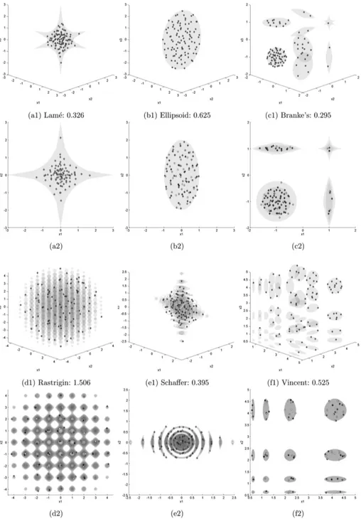
The difficulty of the level set benchmark depends on the level set shapes and their sizes. In general small objects are more difficult to locate, which leads to an increase in difficulty for the benchmark. The same applies for thin parts or acute angles in an object, which add a challenge when locally exploring a feasible com-ponent. If a level set has disjoint parts, it is expected that the algorithm should settle at least one solution on each disjoint part, unless the approximation set size is smaller than the amount of disjoint parts. Many of the chosen complex shape level sets have an exponential growth in the number of their disconnected component when increasing the dimensionality of the level set benchmark. Hav-ing large distances between the disjoint parts can serve as a way to test the global search capabilities of the algorithm. To this end, the difficulty of the level set benchmarks has been tailored according to the philosophy of the ELSA algo-rithm to not consider points in the exterior of the approximation set. Therefore, we avoid components of measure zero. The shape of the level sets can be seen in Fig.1.
5
Experimental Analysis
The experiments with ELSA consist of two main parts: First part shows that implementing both global and local search is essential for black box level set benchmarks. The importance of mixed mutation strategy is measured by com-paring differentν values for ELSA on 3D Ellipsoid and Vincent level set bench-mark for two differentσstep-sizes (results presented in Table1); In the second part, the importance of choosing the right σ step-size is highlighted, this is seen from the experiments of ELSA on all benchmarks. These experiments show the robustness of ELSA with different σstep-sizes on 3D and 10D benchmarks (Tables2 and3, respectively), whereν is set to 0.5 (a recommended parameter value derived from the mixed mutation strategy experiments). Finally, Table4 presents a comparison on the amount of evaluations to yield a population that solely consists of feasible solutions, with respect to different step-sizes, for 3D and 10D benchmarks. The Monte Carlo Search (MCS) is included as a reference algorithm configuration in all the experiments. ELSA can easily be transformed into the MCS approach by settingν to 0 (σis irrelevant as the algorithm never produce children through parent perturbation).
for all experiments. Each configuration has been run 40 times. Several σ step-sizes are to be defined to use in ELSA. The generic form for the σstep-size is described below, wheredis the dimension:
σ= ω·mean(x
max−xmin)
√
d
√
dis derived from the longest diagonal of ann-dimensional hypercube. The chosenω values for theσstep-sizes are 1, 0.1, 0.01, and 0.001 (different magni-tudes of 10). 3D Ellipsoid and 3D Vincent are used as the level set benchmarks to compare the results for mixed mutation strategy. They represent the core oppo-sites of having a non-disjoint level set with Ellipsoid versus the multisegmented Vincent level set. The chosenν values are 0, 0.25, 0.5, 0.75, and 1.
The following objectives are used for the comparison of the results:
– Diversity: The Quality Indicator value of the final population.
– EvalF easible: The amount of evaluations it takes to yield a population that
solely consists of feasible solutions.
– Coverage of the final population on the level set determined by human observation.
Table1 allows us to reason about the effect ν has in scenarios of small and big step-sizes, for single level set (Ellipsoid) and multiple level set (Vincent) problems. For the Ellipsoid problem with ω= 0.1, we see that the higher theν value the better the diversity yielded with GI+Πand SP+. This behavior is mainly explained by the fact that Ellipsoid is a single level set problem. In Vincent problem with ω = 0.1 both GI+Π and SP+ indicators show that intermedium values of ν (0.25 and 0.5) perform better than extreme ones such as 0 and 1 (best from worst for GI+Π and SP+: 0.25, 0.5, 0, 0.75, 1, with ν = 1 being significantly worse).
For ω = 0.01, both GI+Π and SP+ indicators in the Ellipsoid problem also reveal that intermedium values of ν such as 0.5 and 0.75 perform better than extreme ones (GI+Π best to worst: 0.5, 0.75, 0.25, 0, 1; and SP: 0.75, 0.5, 0.25, 0, 1). A similar conclusion can be made for the Vincent problem withω= 0.01, intermedium values of 0.25 and 0.5 ofνallow for best GI+Πand SP+results (best to worst, GI+Π and SP+: 0.25, 0.5, 0, 0.75, 1).
Table 1.The diversity of the final populations from ELSA withω= 0.1 andω= 0.01 forσstep-size and differentνvalues on selected 3D level set benchmarks.
ν= 0 ν= 0.25 ν= 0.5 ν= 0.75 ν= 1 mean std mean std mean std mean std mean std
Ellipsoid (ω= 0.1)
GI+
Π 0.592 0.004 0.613 0.005 0.625 0.004 0.631 0.005 0.637 0.004
SP+ 99.198 0.029 99.327 0.021 99.381 0.016 99.413 0.015 99.439 0.012
Vincent (ω= 0.1)
GI+Π 0.518 0.015 0.532 0.013 0.525 0.016 0.485 0.021 0.355 0.030
SP+ 98.736 0.243 98.953 0.125 98.920 0.202 98.665 0.379 94.613 2.098 Ellipsoid
(ω= 0.01)
GI+Π 0.592 0.004 0.637 0.006 0.647 0.005 0.641 0.007 0.504 0.050
SP+ 99.198 0.029 99.444 0.022 99.498 0.016 99.510 0.017 99.091 0.411
Vincent (ω= 0.01)
GI+Π 0.518 0.015 0.562 0.015 0.541 0.019 0.440 0.025 0.178 0.028
SP+ 98.736 0.243 99.088 0.182 98.948 0.232 97.665 0.621 70.054 9.182
Experiment results in Table2 show that ELSA is able to consistently find entirely feasible populations with high diversity on all 3D level set benchmarks for almost all the tested σ step-sizes. Even MCS can produce relatively good results with the exception of Lam´e benchmark which proves to be too difficult to find feasible solutions with purely random search. The results from ω = 1 resemble the results of MCS, thus it can be considered a too large step-size. ELSA withω= 0.1 and ω= 0.01 are most successful at finding diverse approx-imation sets, where the results with ω= 0.1 have noticeably better diversity in 3D Schaffer. Results from w= 0.001 however show a decline in diversity which indicates that thisσstep-size is too small for the level set benchmarks. Similar patterns between the different step-sizes are reflected in the 10D level set bench-marks (See Table3). Again, the configurations withω = 0.1 and ω = 0.01 are observed to be most suited in general for these type of black-box level set bench-marks. However, the limitations of ELSA are revealed in higher dimensions as it struggles with finding an entirely feasible set for Lam´e, Rastrigin and Schaffer regardless of σstep-size. MCS and ELSA withω= 1 are the most severe cases whereby they cannot even find any entirely feasible populations. For the other 10D benchmarks, ELSA withω= 0.1 orω= 0.01 find diverse populations where the results from Solow-Polasky on Ellipsoid and Hollow Sphere are near optimal in measurement.
Table 2.The diversity of the final populations from the tested algorithm configurations on the 3D level set benchmarks.
MCS ω= 1 ω= 0.1 ω= 0.01 ω= 0.001 mean std mean std mean std mean std mean std
Lam´e GI+Π−15.411 41.893 −6.820 23.989 0.326 0.006 0.284 0.015 0.121 0.022 SP+ 68.961 2.642 67.740 2.609 86.442 0.448 85.503 1.103 57.155 4.318
Ellipsoid GI+Π 0.592 0.004 0.593 0.006 0.625 0.004 0.647 0.005 0.594 0.007 SP+ 99.198 0.029 99.192 0.035 99.381 0.016 99.498 0.016 99.170 0.045
Hollow GI+Π 0.575 0.007 0.576 0.005 0.614 0.005 0.639 0.007 0.576 0.007 SP+ 99.131 0.043 99.144 0.038 99.362 0.016 99.504 0.020 99.091 0.065
Double GI+Π 0.413 0.006 0.413 0.007 0.463 0.003 0.464 0.007 0.396 0.010 SP+ 95.128 0.203 95.049 0.203 96.709 0.077 97.059 0.107 94.230 0.468
Branke’s GI+Π 0.254 0.009 0.260 0.006 0.295 0.007 0.291 0.011 0.205 0.019 SP+ 80.179 1.267 80.364 1.550 86.537 0.731 86.173 1.627 71.108 3.214
Rastrigin GI+Π 1.549 0.014 1.552 0.019 1.506 0.023 1.563 0.025 1.493 0.022 SP+ 100.000 0.000 100.000 0.000 100.000 0.000 100.000 0.000 100.000 0.000
Schaffer GI+Π 0.302 0.016 0.307 0.012 0.395 0.005 0.302 0.016 0.190 0.032 SP+ 84.973 1.839 84.918 1.991 93.275 0.434 86.424 1.767 71.024 4.023
Vincent GI+Π 0.518 0.015 0.514 0.019 0.525 0.016 0.541 0.019 0.444 0.022 SP+ 98.736 0.243 98.716 0.212 98.920 0.202 98.948 0.232 97.132 0.571
Table 3.The diversity of the final populations from the tested algorithm configurations on the 10D level set benchmarks.
MCS ω= 1 ω= 0.1 ω= 0.01 ω= 0.001
mean std mean std mean std mean std mean std
Lam´e GI+Π−2199.11 3.39−2182.17 3.21−1922.81 11.17 −1422.44 859.12 −2067.21 36.38 SP+ −301.53 3.79 −284.76 2.86 −32.02 1.43 −41.11 48.43 −174.82 31.63 Ellipsoid GI+Π−2027.30 15.73−1980.68 26.12 1.663 0.014 1.242 0.076 0.177 0.045
SP+ −139.80 5.24 −104.30 7.35 100.000 0.000 100.000 0.000 27.434 14.023 Hollow GI+Π−1944.75 19.53−1872.49 38.62 1.760 0.005 1.502 0.023 0.215 0.041 SP+ −68.39 4.55 −44.02 4.14 100.000 0.000 100.000 0.000 34.293 9.441 Double GI+Π−2586.90 12.45−2467.93 17.08 0.966 0.032 0.945 0.008 −402.69 791.54
SP+ −692.29 15.41 −571.12 13.84 99.948 0.018 99.946 0.002 −0.89 39.49 Rastrigin GI+Π−7355.82 98.02−7144.56 82.24−3095.72 546.12−2101.94 1743.26 −1985.23 1837.74 SP+−4531.24 71.23−4324.87 80.48 −600.63 286.13 −281.08 526.95 −494.81 672.37 Schaffer GI+Π−2439.64 8.68−2403.24 9.41−1743.84 41.45 −2118.51 95.64 −2114.59 70.52 SP+ −859.49 7.69 −824.42 9.42 −175.86 52.09 −526.95 123.59 −553.91 64.94 Vincent GI+Π−1210.98 56.09−1174.72 62.49 0.943 0.102 0.726 0.112 0.218 0.029
SP+ 9.88 3.63 13.87 3.56 99.933 0.041 98.281 2.331 51.121 9.313
Table 4. EvalF easible of the results from the tested algorithm configurations. EvalF easible is calculated as the average of the results from GI+Π and SP+ combined. The “-” symbol marks a configuration that contains at least one population that does not solely consist of feasible solutions.
3D 10D
MCS ω= 1 ω= 0.1 ω= 0.01 ω= 0.001ω= 0.1 ω= 0.01 ω= 0.001 mean std mean std mean std mean std mean std mean std mean std mean std
Lam´e - - - - 1067 113 911 137 957 238 - - - -Ellipsoid 1030 101 1044 93 468 40 454 49 456 49 3045 493 9022 2436 40474 17868
Hollow 1279 122 1252 119 539 46 492 46 488 60 2715 362 7852 2245 29867 12113
Double 2570 278 2542 255 686 68 622 75 642 100 4377 473 13679 3507 -
-Branke’s 4488 468 4105 419 969 89 764 109 758 127
Rastrigin 1043 106 1062 93 710 66 465 44 453 42 - - - -Schaffer 6316 663 6247 586 1101 120 862 135 833 143 - - -
-Vincent 2852 309 2843 283 1086 91 659 83 656 77 3152 534 2694 674 5946 2991
tendency for solutions to reside on the boundary of the level set which is not always a desired behavior when taking practical applications into account. While figures labeled with 1 (for example a1) represent 3D plots of the level sets, figures labeled with 2 represent a 2D projection of the 3D plots (for example a2). The level sets are depicted in light gray and are semi-transparent. In the 3D view, the RGB-value (converted into gray scale) of a solution maps to the (x1, x2, x3 )-coordinate of the solution with respect to the search space. In the orthographic view, gray scale coding is used to determine the location of the solution with respect to thex3-axis.
Fig. 1.Visualization of results on 3D benchmark achieved with GI+
6
Summary and Outlook
The current study shows that a mixed strategy of random reinitialization and parent-based mutation is preferable to using only one of these strategies, because it allows to explore and to refine at the same time, thereby minimizing the risk that a component of the level set is overlooked. This mixed strategy might be considered preferable, as we lose performance for the sake of reliability.
In contrast to previous work where only 2D problems were addressed, in our study ELSA performance is assessed for low (3D) and high dimensional level sets (10D). This study allowed to conclude that step size parameter is crucial (specially in higher dimensions) to get both good coverage and to find the components of the level set. Automatic adaptation of the step size (Self-adaptiveσ) should be developed to adapt the algorithm parameters to problem specific properties.
Although ELSA has revealed very good performance in simple shape bench-marks such as Ellipsoid for low and high dimensions, there is still space for improvement in shapes with acute parts such as Lam´e, Rastrigin and Schaffer, specially in high dimensions. To this end, new selection and cross-over operations can be designed for ELSA.
There are still some ways that can be tried to improve the performance of ELSA: The current version of ELSA does not utilize cross-over, that might help to improve the level set coverage (close gaps). However, it might also be dis-ruptive, when applied to individuals from different components of the level set. Moreover, creating more than one children or introduction of mating selection could be beneficial for improving the quality of results, but would also signifi-cantly increase computational costs of an iteration.
In contrast to evolutionary algorithms AIS feature a variable population size and they also have some inherent mechanisms for diversity maintenance, which makes them a promising technique for level set approximation [CZ06].
References
[Bra98] Branke, J.: Creating robust solutions by means of evolutionary algo-rithms. In: Eiben, A.E., B¨ack, T., Schoenauer, M., Schwefel, H.-P. (eds.) PPSN 1998. LNCS, vol. 1498, pp. 119–128. Springer, Heidelberg (1998). doi:10.1007/BFb0056855
[CZ06] Coelho, G.P., Von Zuben, F.J.: omni-aiNet: an immune-inspired approach for omni optimization. In: Bersini, H., Carneiro, J. (eds.) ICARIS 2006. LNCS, vol. 4163, pp. 294–308. Springer, Heidelberg (2006). doi:10.1007/ 11823940 23
[EDK13] Emmerich, M.T.M., Deutz, A.H., Kruisselbrink, J.W.: On quality indi-cators for black-box level set approximation. In: Tantar, E., Tantar, A.-A., Bouvry, P., Del Moral, P., Legrand, P., Coello, C.A.C., Sch¨utze, O. (eds.) EVOLVE-A Bridge Between Probability, pp. 157–185. Set Oriented Numerics and Evolutionary Computation. Springer, Heidelberg (2013) [Kru12] Kruisselbrink, J.W.: Evolution strategies for robust optimization. Ph.D.
thesis, Leiden Institute of Advanced Computer Science (LIACS), Faculty of Science, Leiden University (2012)
[NE15] Nezhinsky, A., Emmerich, M.T.M.: Parameter identification of stochastic gene regulation models by indicator-based evolutionary level set approx-imation. In: Proceedings of EVOLVE - A Bridge Between Probability, Set-Oriented Numerics, and Evolutionary Computation, Iasi, June 2015. Springer, Heidelberg (2015, in print)
[PCWB00] Parmee, I.C., Cvetkovi´c, D., Watson, A.H., Bonham, C.R.: Multiobjective satisfaction within an interactive evolutionary design environment. Evol. Comput.8(2), 197–222 (2000)
[Set99] Sethian, J.A.: Level Set Methods and Fast Marching Methods: Evolv-ing Interfaces in Computational Geometry, Fluid Mechanics, Computer Vision, and Materials Science, vol. 3. Cambridge University Press, Cam-bridge (1999)
[SPB93] Solow, A., Polasky, S., Broadus, J.: On the measurement of biological diversity. J. Environ. Econ. Manag.24(1), 60–68 (1993)
[UBT10] Ulrich, T., Bader, J., Thiele, L.: Defining and optimizing indicator-based diversity measures in multiobjective search. In: Schaefer, R., Cotta, C., Kolodziej, J., Rudolph, G. (eds.) PPSN 2010. LNCS, vol. 6238, pp. 707– 717. Springer, Heidelberg (2010). doi:10.1007/978-3-642-15844-5 71
[UT11] Ulrich, T., Thiele, L.: Maximizing population diversity in single-objective optimization. In: Proceedings of the 13th Annual Conference on Genetic and Evolutionary Computation, pp. 641–648. ACM (2011)
[vdB13] van der Burgh, B.: An evolutionary algorithm for finding diverse sets of molecules with user-defined properties. Technical report (2013)
[vdGSB08] van der Goes, V., Shir, O.M., B¨ack, T.: Niche radius adaptation with asymmetric sharing. In: Rudolph, G., Jansen, T., Beume, N., Lucas, S., Poloni, C. (eds.) PPSN 2008. LNCS, vol. 5199, pp. 195–204. Springer, Heidelberg (2008). doi:10.1007/978-3-540-87700-4 20