HAL Id: hal-01412823
https://hal-mines-paristech.archives-ouvertes.fr/hal-01412823
Submitted on 19 Mar 2018
HAL
is a multi-disciplinary open access
archive for the deposit and dissemination of
sci-entific research documents, whether they are
pub-lished or not. The documents may come from
teaching and research institutions in France or
abroad, or from public or private research centers.
L’archive ouverte pluridisciplinaire
HAL, est
destinée au dépôt et à la diffusion de documents
scientifiques de niveau recherche, publiés ou non,
émanant des établissements d’enseignement et de
recherche français ou étrangers, des laboratoires
publics ou privés.
An intercomparison of remote sensing river discharge
estimation algorithms from measurements of river
height, width, and slope
M. Durand, C. Gleason, Pierre-André Garambois, D. Bjerklie, L.C. Smith, H
Roux, E. Rodriguez, P. D. Bates, T.M. Pavelsky, Jérôme Monnier, et al.
To cite this version:
M. Durand, C. Gleason, Pierre-André Garambois, D. Bjerklie, L.C. Smith, et al..
An
in-tercomparison of remote sensing river discharge estimation algorithms from measurements of
river height, width, and slope.
Water Resources Research, American Geophysical Union, 2016,
52 (6), pp.4527-4549.
�https://agupubs.onlinelibrary.wiley.com/doi/full/10.1002/2015WR018434�.
Open Archive TOULOUSE Archive Ouverte (OATAO)
OATAO is an open access repository that collects the work of Toulouse researchers and
makes it freely available over the web where possible.
This is an author-deposited version published in :
http://oatao.univ-toulouse.fr/
Eprints ID : 19569
To link to this article
: DOI:10.1002/2015WR018434
URL :
http://dx.doi.org/10.1002/2015WR018434
To cite this version
: Durand, Michael and Gleason, Colin and
Garambois, Pierre-André,… [et al.]
An intercomparison of remote
sensing river discharge estimation algorithms from measurements of
river height, width, and slope.
(2016) Water Resources Research, vol.
52 (n° 6). pp. 4527-4549. ISSN 0043-1397
An intercomparison of remote sensing river discharge
estimation algorithms from measurements of river height,
width, and slope
M. Durand1, C. J. Gleason2, P. A. Garambois3, D. Bjerklie4, L. C. Smith5, H. Roux6,7, E. Rodriguez8,
P. D. Bates9, T. M. Pavelsky10, J. Monnier11, X. Chen12, G. Di Baldassarre13, J.-M. Fiset14, N. Flipo15,
R. P. d. M. Frasson1, J. Fulton16, N. Goutal17, F. Hossain18, E. Humphries10, J. T. Minear19,
M. M. Mukolwe20, J. C. Neal9, S. Ricci21, B. F. Sanders22, G. Schumann9,23, J. E. Schubert22, and
L. Vilmin15
1School of Earth Sciences and Byrd Polar and Climate Research Center, Ohio State University, Columbus, Ohio, USA, 2
Department of Civil and Environmental Engineering, University of Massachusetts, Amherst, Massachusetts, USA,3ICUBE, Fluid Mechanics Team, Department of Civil Engineering, INSA Strasbourg, Strasbourg, France,4Connecticut Water Science Center, USGS, Hartford, Connecticut, USA,5Department of Geography, University of California, Los Angeles, California, USA,6Universite de Toulouse, INPT, UPS, Institut de Mecanique des Fluides de Toulouse, Toulouse, France,7CNRS, IMFT, Toulouse, France,8Jet Propulsion Laboratory, NASA, Pasadena, California, USA,9School of Geographical Sciences, University of Bristol, Bristol, UK,10Department of Geological Sciences, University of North Carolina, Chapel Hill, North Carolina, USA,11INSA, Institut de Mathematiques de Toulouse, Toulouse, France,12NOAA/NWS/Ohio River Forecast Center, Wilmington, Ohio, USA,13Department of Earth Sciences, Uppsala University, Uppsala, Sweden,14Environment Canada, Quebec, Canada,15Centre de Geosciences, MINES ParisTech, PSL Research University, Paris, France,16USGS Colorado Water Science Center, Lakewood, Colorado, USA,17St Venant Lab Hydraul and EDF R&D, University of Paris-Est, France,18Department of Civil and Environmental Engineering, University of Washington, Seattle, Washington, USA, 19USGS Geomorphology and Sediment Transport Lab, Golden, Colorado, USA,20UNESCO-IHE Institute for Water Education, Delft, Netherlands,21CECI, CERFACS/CNRS, Toulouse, France,22Department of Civil and Environmental Engineering, University of California, Irvine, California, USA,23Remote Sensing Solutions, Inc., Monrovia, California, USA
Abstract
The Surface Water and Ocean Topography (SWOT) satellite mission planned for launch in 2020 will map river elevations and inundated area globally for rivers>100 m wide. In advance of this launch, we here evaluated the possibility of estimating discharge in ungauged rivers using synthetic, daily ‘‘remote sensing’’ measurements derived from hydraulic models corrupted with minimal observational errors. Five discharge algorithms were evaluated, as well as the median of the five, for 19 rivers spanning a range of hydraulic and geomorphic conditions. Reliance upon a priori information, and thus applicability to truly ungauged reaches, varied among algorithms: one algorithm employed only global limits on velocity and depth, while the other algorithms relied on globally available prior estimates of discharge. We found at least one algorithm able to estimate instantaneous discharge to within 35% relative root-mean-squared error (RRMSE) on 14/16 nonbraided rivers despite out-of-bank flows, multichannel planforms, and backwater effects. Moreover, we found RRMSE was often dominated by bias; the median standard deviation of relative residuals across the 16 nonbraided rivers was only 12.5%. SWOT discharge algorithm progress is therefore encouraging, yet future efforts should consider incorporating ancillary data or multialgorithm synergy to improve results.1. Introduction
Rivers link atmospheric, terrestrial, and oceanic processes and route approximately two fifth of the global total rainfall over land back into the ocean [V€orosmarty et al€ ., 2000;Oki and Kanae, 2006]. In doing so, they represent an important resource for agriculture and urban development as well a major hazard during flood events. In these contexts, accurate estimation of river discharge (also ‘‘streamflow’’ or ‘‘runoff,’’ units of vol-ume per unit time) is vital, as it quantifies the amount of water resources available for human consumption, defines the quantity of water that must be routed during a flood event, and indicates overall watershed response to atmospheric forcing. Despite its importance, our knowledge of global river discharge is
Key Points:
SWOT discharge algorithms were tested on synthetic observations for 19 rivers
Algorithms accurately characterized temporal dynamics of river discharge
surprisingly poor. This lack of knowledge represents an acute problem, given the possible acceleration of the water cycle due to global warming [Huntington, 2006]. Improved river discharge estimates, with greater spatial coverage of the global system of rivers, are needed to develop process-based scientific understand-ing of runoff at large spatial scales (i.e., how water is routed into and through rivers) and to calibrate and constrain hydrologic models to forecast effects of future changes in the terrestrial hydrologic cycle. The forthcoming Surface Water and Ocean Topography (SWOT) mission measurements of river water surface elevation (WSE), top width, and free-surface slope may allow periodic estimation of river discharge for all rivers wider than 100 m, with a goal of estimating discharge for rivers wider than 50 m [Biancamaria et al., 2015;Pavelsky et al., 2014]. Accurate discharge estimates from these measurements would enable tremen-dous advances in global hydrologic studies.
Given that discharge is the product of flow area and velocity, in situ measurement of river discharge requires spatially explicit measurements of the vertical velocity profile using a current meter in a transect orthogonal to river flow [Turnipseed and Sauer, 2010]. While in situ measurements of discharge can be highly accurate, they are time consuming and impractical for continuous monitoring. Such monitoring is often achieved via river gauges that leverage periodic, simultaneous measurements of river stage (height above some arbitrary datum) and discharge to develop a ‘‘rating curve.’’ With this rating curve defined, mea-surement of river stage is performed (usually) by pressure transducer, allowing for nearly continuous predic-tion of river discharge via the rating curve.
SWOT-based discharge will never be a replacement for in situ discharge measurements. SWOT overpasses have a 21 day cycle, and will sample midlatitude locations irregularly in time approximately 3 times per cycle [Biancamaria et al., 2015], rather than nearly continuously, as in a gauge estimate. While this is adequate for addressing scientific questions related to the global water cycle, it is inadequate for many local-scale questions on rivers where SWOT may not fully observe temporal dynamics [Biancamaria et al., 2010], and for which data are often required at subhourly time scales. Additionally, SWOT discharge esti-mates are not expected to be as precise as gauged discharge. On the other hand, the spatially continuous nature of the SWOT measurements will provide data in currently ungauged basins as well as measurements of spatially distributed phenomena such as the propagation of floodwaves along rivers [Durand et al., 2010;
Pavelsky et al., 2014;Paiva et al., 2015]. SWOT will also complement river discharge modeling. Global water balance models use climate forcings to determine river runoff, but rely on gauges for parameter tuning [Hunger and Doell, 2008]. SWOT can provide discharge estimates at continental scale in order to help reduce current model annual runoff errors that range from 10 to 80%, and are commonly 40% [Oki et al., 1999; Raw-lins et al., 2003;Widen-Nilsson et al., 2007;Gosling and Arnell, 2011]. SWOT will complement both gauges and water balance modeling and can form a key component in understanding the global water budget—if discharge algorithms with sufficient accuracy can be developed.
River discharge estimation from satellite remote sensing of river hydraulic variables including width, stage, slope, surface velocity, and channel pattern has been explored and discussed in recent decades [Smith et al., 1996;Smith, 1997;Bjerklie et al., 2003;Kouraev et al., 2004;Bjerklie et al. 2005a;Dingman and Bjerklie, 2006; Bjer-klie, 2007;Birkinshaw et al., 2010;Michailovsky et al., 2012]. In some of these studies, altimetry measurements were utilized to estimate discharge with a rating curve available from an in situ discharge gage [e.g.,Kouraev et al., 2004]. Other studies envisioned estimating discharge in ungauged rivers, and utilized traditional flow laws where only a subset of the hydraulic quantities specified by the flow laws were observed remotely, and pointed to the need for estimating the unobserved variables, such as roughness coefficient or river bathymetry [e.g.,Bjerklie et al., 2003].Roux and Dartus[2005, 2008] proposed methods for estimating unobserved hydraulic parameters from water surface width observations, on a synthetic case and using observed maximum flood extents.Roux and Dartus[2006] estimated a synthetic flood hydrograph by minimizing the distance between flood extent observations and 1-D model outputs, assuming the channel geometry and roughness are known with a given uncertainty.Lai and Monnier[2009] assimilated water levels into a 2-D model and demonstrated that the inflow hydrograph could be estimated. The anticipated SWOT data have sparked development of new efforts to develop discharge estimation methods (discussed in detail, below), which draw from these previous studies and decades of heritage in the fields of hydraulics, remote sensing, and fluvial geomorphology.
SWOT output (averaged observations of WSE, slope and inundation area over10 km reaches [Fjortoft et al., 2014]) to estimate river discharge. Algorithms include the previously published at-many-stations hydraulic geometry (AMHG) method [Gleason and Smith, 2014;Gleason et al., 2014], GaMo [Garambois and Monnier, 2015], MetroMan [Durand et al., 2014], and the novel mean flow and geomorphology (MFG) and the mean flow and constant roughness (MFCR) algorithms, in addition to an ensemble median product. We use synthetic daily observations of WSE and width generated from hydrodynamic models for 19 rivers cov-ering a wide range of hydrologic regimes as a stand-in for SWOT data. We first describe each of the algo-rithms in detail and then compare their estimation results before concluding with a summary of algorithm strengths and weakness and a prognosis for the future SWOT mission.
2. Experiment Design
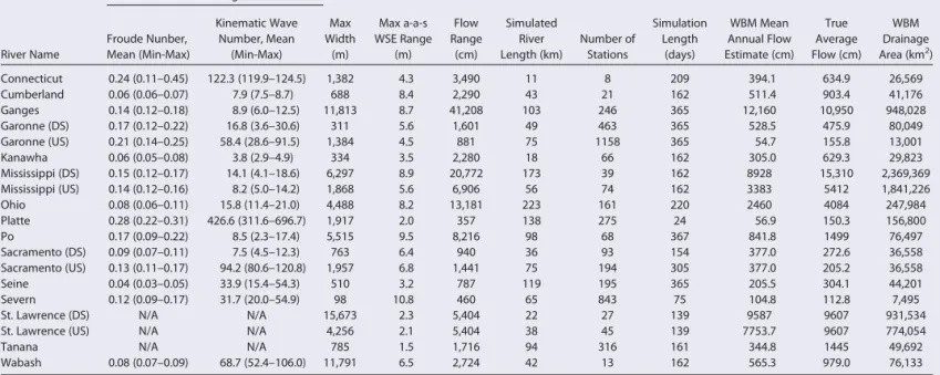
We used hydrodynamic model output from 19 rivers to assess algorithm performance in this study (Figure 1). For each river, daily synthetic measurements of water surface slope, elevation, and top width
Figure 1.Map showing hydraulic model locations. The rivers shown are those estimated to be greater than 50 m in width, slightly adapted from the analysis ofPavelsky et al. [2014]. (a) Platte. (b) Tanana. (c) Seine. (d) Severn. (e) Garonne—Upstream. (f) Garrone—Downstream. (g) Cumberland. (h) Kanawha. (i) Sacramento—Upstream. (j) Sacramento—Downstream. (k) Connecticut. (l) Wabash. (m) Ohio. (n) Mississippi—Upstream. (o) Mississippi—Downstream. (p) Saint Lawrence—Upstream. (q) Saint Lawrence—Downstream. (r) Po. (s) Ganges.
Table 1.Modeling Platform and Reference for Each Hydraulic Model, Along With the Dates Simulated in Each Model
River Name Model Reference Dates Simulated
Connecticut HEC-RAS 31 May 2011 to 27 Dec 2011
Cumberland HEC-RAS Adams et al. [2010] 1 Jan 2012 to 30 Jun 2012
Ganges HEC-RAS Siddique-E-Akbor et al. [2011] andMaswood
and Hossain[2015]
1 Jan 2002 to 31 Dec 2002
Garonne (DS) Mascaret Besnard and Goutal[2008] andLarnier[2010] 1 Jan 2010 to 31 Dec 2010
Garonne (US) HEC-RAS 1 Jan 2010 to 31 Dec 2010
Kanawha HEC-RAS Adams et al. [2010] 1 Jan 2012 to 30 Jun 2012
Mississippi (DS) HEC-RAS Adams et al. [2010] 1 Jan 2012 to 30 Jun 2012
Mississippi (US) HEC-RAS Adams et al. [2010] 1 Jan 2012 to 30 Jun 2012
Ohio HEC-RAS Adams et al. [2010] 1 Jan 2012 to 30 Jun 2012
Platte BreZo (2-D) Schubert et al. [2015] 13 Sep 2013 to 7 Oct 2013
Po HEC-RAS Di Baldassarre et al. [2009] 2 Feb 2002 to 3 Feb 2003
Sacramento (DS) HEC-RAS Rogers[2014] 1 Feb 2009 to 4 Jul 2009
Sacramento (US) HEC-RAS Rogers[2014] 1 Jan 2009 to 12 Sep 2009
Seine ProSe Vilmin et al. [2015] 1 Aug 2009 to 31 Jul 2009
Severn LISFLOOD-FP Neal et al. [2015] 2 Jun 2007 to 31 Aug 2007
St. Lawrence (DS) H2D2 (2-D) Heniche et al. [2000] 27 Apr 2013 to 16 Oct 2013 St. Lawrence (US) H2D2 (2-D) Heniche et al. [2000] 27 Apr 2013 to 16 Oct 2013 Tanana LISFLOOD-FP (2-D) Humphries et al.[2014] 24 May 2013 to 30 Oct 2013
corresponding to different flows were generated by a hydraulic model forced by in situ bathymetry, simu-lated or gauged inflows at the top of the reach, and downstream water elevation boundary conditions. The philosophy of the experiment design was to evaluate discharge estimation under essentially ideal condi-tions: e.g., daily observations were utilized, although SWOT will measure less frequently—seeBiancamaria et al. [2015] for discussion of SWOT space-time coverage. Moreover, only minimal random measurement errors were added to the height, width, and slope time series. Future studies will build upon what is shown here to examine the effect of SWOT measurement errors, and space-time sampling.
In some cases, multiple models on the same river have been used (e.g., an upstream and downstream reach of the Garonne River are both included); each of the 19 is hereafter referred to as ‘‘rivers’’ as each is an inde-pendent set of data representing a different range of hydraulic conditions that can be used to evaluate algorithm performance. Outputs from six different modeling platforms were used in this study, including HEC-RAS (12 rivers) [Brunner, 2010], LISFLOOD-FP (2 rivers) [Bates et al., 2010], H2D2 (2 rivers) [Heniche et al., 2000], BreZo (1 river) [Kim et al., 2014], Mascaret (1 river) [Goutal and Maurel, 2002], and ProSe (1 river) [ Vil-min et al., 2015]. Table 1 provides references for each individual model, and Table 2 summarizes simulation time, reach lengths, and hydraulic characteristics for the 19 rivers in this study.
The models used here were developed for purposes other than those in this study, and so each uses differ-ent procedures to generate the hydraulic variables of interest and each is run with differdiffer-ent spatial and tem-poral resolutions. A full discussion of the differing model solution schemes and solvers is outside the scope of this paper, and the interested reader is referred to the citations for each model given above and in Tables 1 and 2 for further information. However, there are a number of core similarities across all of the models. All of the models represented study reaches with discrete units: either cross sections perpendicular to flow or 2-D grid elements. At each of these units, the models solve for conservation of energy or momentum, using variants of either the 1-D or 2-D St. Venant or shallow water equations. Note that all models were built using field measurements of bathymetry. In all cases, flow boundary conditions from a stream gauge were imposed at the top of the reach and a water surface elevation or ‘‘free-surface slope’’ boundary condition imposed at the downstream of the reach, allowing the models to apply their particular solver to attain a sta-ble solution for the hydraulics of each solution unit. Models were calibrated by adjusting the roughness coefficient in order to match water surface elevation and discharge measurements. These numerical solu-tions to the conservation equasolu-tions, coupled with the model’s geometric representation of the river chan-nel, yield the hydraulic parameters of interest for this study at each unit: water surface elevation, top width, and water surface slope. In the case of multiple channels, hydraulic quantities were summed across chan-nels to derive a single value, which matchesSchubert et al.’s [2015] ‘‘integrated’’ form for multiple channels.
Table 2.Summary of the Hydraulic Model Output Used for Each River
River Name Reach Average Max Width (m) Max a-a-s WSE Range (m) Flow Range (cm) Simulated River Length (km) Number of Stations Simulation Length (days) WBM Mean Annual Flow Estimate (cm) True Average Flow (cm) WBM Drainage Area (km2) Froude Nunber,
Mean (Min-Max)
Kinematic Wave Number, Mean
(Min-Max)
Connecticut 0.24 (0.11–0.45) 122.3 (119.9–124.5) 1,382 4.3 3,490 11 8 209 394.1 634.9 26,569
Cumberland 0.06 (0.06–0.07) 7.9 (7.5–8.7) 688 8.4 2,290 43 21 162 511.4 903.4 41,176
Ganges 0.14 (0.12–0.18) 8.9 (6.0–12.5) 11,813 8.7 41,208 103 246 365 12,160 10,950 948,028
Garonne (DS) 0.17 (0.12–0.22) 16.8 (3.6–30.6) 311 5.6 1,601 49 463 365 528.5 475.9 80,049
Garonne (US) 0.21 (0.14–0.25) 58.4 (28.6–91.5) 1,384 4.5 881 75 1158 365 54.7 155.8 13,001
Kanawha 0.06 (0.05–0.08) 3.8 (2.9–4.9) 334 3.5 2,280 18 66 162 305.0 629.3 29,823
Mississippi (DS) 0.15 (0.12–0.17) 14.1 (4.1–18.6) 6,297 8.9 20,772 173 39 162 8928 15,310 2,369,369
Mississippi (US) 0.14 (0.12–0.16) 8.2 (5.0–14.2) 1,868 5.6 6,906 56 74 162 3383 5412 1,841,226
Ohio 0.08 (0.06–0.11) 15.8 (11.4–21.0) 4,488 8.2 13,181 223 161 220 2460 4084 247,984
Platte 0.28 (0.22–0.31) 426.6 (311.6–696.7) 1,917 2.0 357 138 275 24 56.9 150.3 156,800
Po 0.17 (0.09–0.22) 8.5 (2.3–17.4) 5,515 9.5 8,216 98 68 367 841.8 1499 76,497
Sacramento (DS) 0.09 (0.07–0.11) 7.5 (4.5–12.3) 763 6.4 940 36 93 154 377.0 272.6 36,558
Sacramento (US) 0.13 (0.11–0.17) 94.2 (80.6–120.8) 1,957 6.8 1,441 75 194 305 377.0 205.2 36,558
Seine 0.04 (0.03–0.05) 33.9 (15.4–54.3) 510 3.2 787 119 195 365 205.5 304.1 44,201
Severn 0.12 (0.09–0.17) 31.7 (20.0–54.9) 98 10.8 460 65 843 75 104.8 112.8 7,495
St. Lawrence (DS) N/A N/A 15,673 2.3 5,404 22 27 139 9587 9607 931,534
St. Lawrence (US) N/A N/A 4,256 2.1 5,404 38 45 139 7753.7 9607 774,054
Tanana N/A N/A 785 1.5 1,716 94 316 161 344.8 1445 49,692
Reaches on the order of 5–10 km were defined based on inflection points in the water surface elevation data; methods to automatically identify optimal reach boundaries are needed, and are currently in develop-ment. Reach-averaged hydraulic quantities were utilized in the Manning’s-based discharge algorithms, while cross-section data were used directly in the hydraulic geometry-based approach. Time series of simu-lated river height, width, and slope for all rivers were produced by adding Gaussian errors with standard deviations of 5 cm, 5 m, and 0.1 cm/km, respectively; time series of height, width, and slope are shown in Figures (2 and 3), and 4, respectively. The error standard deviations are admittedly somewhat arbitrary, but were chosen to be small enough to resolve temporal variations visible in Figures 2–4.
Hydraulic regime of each river reach was characterized by two nondimensional numbers: the Froude number and the kinematic wave number, as defined byVieira[1983], and used, e.g., byTrigg et al. [2009]. These nondimensional numbers were calculated for each day for each reach, then averaged in time for each reach. The mean Froude and kinematic wave numbers across all reaches, as well as the minimum and maximum values across all reaches, are shown in Table 2 for each river. Based on comparison with the regime diagram shown inVieira[1983], the hydraulics of nearly all reaches can, perhaps unsurpris-ingly, be considered to be diffusive. The only river that can be considered kinematic is the Platte River, which exhibited both the highest average Froude and kinematic wave numbers (0.28 and 426.6, respec-tively). All reaches exhibit subcritical and gradually varied flow, and no reach showed fully dynamic wave behavior.
While each data set corresponds to a particular reach of a real-world river, our use of simulated inflows and often sampled (rather than acquired via side-scan sonar) or simplified channel and floodplain geometry results in model outputs that may not necessarily represent true hydrologic conditions for each reach: these data are model-simulated representations of fluvial behavior rather than observations. This is an important distinction for this study, as using these model outputs allowed us a large degree of control over algorithm inputs and allowed us the ability to test algorithm performance without consid-ering the effect of measurement error or noise on the data. Further studies utilizing field data and air-borne swath altimetry are in process. Despite this caveat, validation and benchmark tests of hydraulic models built, calibrated, and validated using field and remotely sensed observations do show surpris-ingly good and consistent performance [e.g.,Hunter et al., 2008], with water elevation predictions accu-rate to<10 cm [e.g.,Jung et al., 2012] and inundation extent prediction accuracies up to 90% [Bates et al., 2006].
The experiment here is purposefully highly restrictive, as every algorithm under consideration was required to use the exact same input data and no river-specific assumptions or ancillary data (aside from mean annual flow, as described below) were allowed. All the discharge algorithms (reporting on a given river) employed identical station data and reach lengths over the same period of record (although note that AMHG operated on station data, whereas the other algorithms utilized reach-averaged data). For the future SWOT mission, and in other river discharge studies, ancillary data will form one of the pillars of discharge estimation: it is foolish to not leverage all available information. However, in this study, we seek to answer the most basic of questions regarding discharge algorithm performance, and therefore to make a fair com-parison all methods are restricted to the same input data. This enables an honest assessment of the base principles of discharge estimation solely from remotely sensed data.
We assessed discharge estimation performance according to a suite of nine error metrics proposed by
3. Discharge Algorithms
Beginning approximately a decade ago, several approaches were developed using virtual SWOT observa-tions to test discharge estimation schemes under the aegis of the SWOT virtual mission.Andreadis et al.
[2007] andBiancamaria et al. [2011] assimilated virtual SWOT observations into a hydraulic model, assuming that river bathymetry and the Manning’s frictionn were known. In further developments, Durand et al. [2008] and Yoon et al. [2012] used assimilation approaches to estimate river bathymetry and discharge simultaneously;nwas assumed to be known a priori [Yoon et al., 2012] or known to vary within a relatively small range [Durand et al., 2008]. The computational burden of these data assimilation schemes and diffi-culty in estimating bathymetry, roughness, and discharge within the assimilation scheme led to a search for simpler methods, which would be more amenable to global application, despite the continued importance of assimilation in regional and local-scale applications.Durand et al. [2010] first showed that river bathyme-try and depth could be estimated without running a hydraulic model via analysis of a virtual SWOT observa-tion time series, if n were assumed known. This represented the first demonstration of river discharge estimation with minimal a priori data requirements. Mersel et al. [2013] then demonstrated that SWOT observations could be used to estimate channel bed elevation, provided observations were made at enough different stages, yielding another means of obtaining prior information. Following these early developments, there are now five proposed algorithms for use in the SWOT mission; the median of these five is evaluated as a sixth algorithm herein. The basics of the algorithms are summarized in Table 3; each algorithm is described below.
3.1. At-Many-Stations Hydraulic Geometry (AMHG)
At-a-station hydraulic geometry (AHG), equations (1)–(3), where a, b, c, f, k, andmare empirical best fit parameters, were first described byLeopold and Maddock[1953], and are an often-used framework in river remote sensing [e.g.,Smith et al., 1996;Smith and Pavelsky, 2008;Pavelsky, 2014]. AMHG is a recently discov-ered geomorphic phenomenon holding that the coefficients and exponents in traditional AHG are stably and predictably related for a given river, thus linking individual cross sections to one another along a river [Gleason and Smith, 2014]. Gleason and Smith found that the relationship between these quantities takes a semilog form, and used in situ measurements of width (w), depth (d), velocity (v), and discharge (Q) to dem-onstrate the phenomenon.Gleason and Wang[2015] further showed that AMHG arises because individual, independent rating curves all pass through the same values of wandQ, given in practice by the spatial modes of time meanwandQat each cross section.
Table 3.Summary of Discharge Algorithms
Algorithm Theoretical Basis Applied Variables From Observation Estimated Variables Variable Estimation Method
AMHG At-many-stations hydraulic geometry
Water surface width (W) a, b aandbare optimized to preserve
continuity between stations using a genetic algorithm GaMo Manning flow
resistance equation (equation (4))
Change in cross-sectional area of flow (dA) computed from the mean width and change in water surface height (dH, stage), water surface slope (S) for several reaches
Flow resistance (n) and cross-sectional area of channel at zero flow (A0)
A0andnare both optimized to preserve continuity between the observed reaches using a constrained, nonlinear steepest-descent optimization
MetroMan Manning flow resistance equation (equation (4))
Change in cross-sectional area of flow
(dA) computed from the mean
width and change in water surface height (dH, stage), water surface slope (S) for several reaches
Flow resistance (n) and cross-sectional area of channel at zero flow (A0)
A0andnare both optimized to preserve continuity between the observed reaches (must be three or more) using the Metropolis algorithm
MFG Manning flow
resistance equation (equation (5))
Water surface width (W), water surface slope (S), and water surface height (H, stage) for the reach
Flow resistance (n) and height (stage) of zero flow (B)
nis estimated from an empirical relation between its mean value and slope, and then adjusted based on an empirical relation between the change in river cross section.Bis calibrated to an estimate of the mean annual discharge for the time series MFCR Manning flow
resistance equation (equation (4))
Water surface width, water surface slope, water surface height (stage) for the reach
Cross-sectional area of channel at zero flow (A0)
w5aQb (1)
d5cQf (2)
v5kQm (3)
The AMHG discharge algorithm’s base assumptions are that AHG parameters are constant in time and that mass is conserved in a reach. Discharge is calculated by estimatingaandbin equation (1) and inverting to solve forQin a pairwise permutation assuming thatQis constant across all pairs. Thus, this algorithm only requires inputs of remotely sensed width at-a-station, which differentiates it from the other methods in this study. From a remotely sensed standpoint, this system is underconstrained even in a mass conserved reach: there are four variables per cross section (i.e.,w,Q,a, andb), and only one of them can be remotely sensed (w). Thus, when assuming cross sections share a common discharge given a time series of width observa-tions, there are always 2Nc11 unknowns forNccross sections. Since AMHG relatesaandbfor a given river, it simplifies the AHG system, and results in two unknowns per cross section:Qand thea/btuple. While this system is still underconstrained, it lends itself to heuristic optimization as it leaves onlyNc11 unknowns perNc cross sections.Gleason and Smith [2014] found a remotely sensed proxy that approximates the AMHG for a river given a time series of remotely sensed river widths, thus allowing AHG simplification with-out any a priori knowledge, and solved for discharge by minimizing flow residuals via genetic algorithm optimization of AHG parameters.Gleason and Wang2015] have since shown that this proxy is spurious and give proposals for its replacement, butGleason and Smith[2014] still reported discharge estimations to within 20–36% relative Root-Mean-Squared Error (RRMSE) for three rivers in their initial demonstration, and
Gleason et al. [2014] performed a thorough sensitivity analysis of the AMHG method for 34 rivers, yielding discharge accuracies between 26 and 41% for most river morphologies using the originally proposed proxy. In this paper, we use the original proxy ofGleason and Smith[2014] to estimate discharge.
Importantly,Gleason et al. [2014] recommended ‘‘global’’ parameterizations of the AMHG method for use in ungauged basins, and we follow these parameters here.Gleason et al. [2014] also showed that rivers in arid regions, braided rivers, and low-brivers (where all AHGbexponents are less than 0.1) reliably resulted in poor discharge inversion. We expect that these same exclusions will apply here, so we also include some ‘‘blind’’ data filters intended to improve AMHG performance. Since equation (1) breaks down during over-bank/floodplain flow, we first filter any widths that are 1–3 standard deviations above the mean, depending on the shape of the distribution of input width data. Second, in order to increase the amount of rivers avail-able to AMHG, we filter out cross sections that have a coefficient of variation (standard deviation divided by mean) in observed widths less than 10%; this is a much less stringent filter than is typically used, although it still results in exclusion of 8 of the 19 rivers by AMHG. Thus, we are able to estimate discharge for some riv-ers whose width data would suggest that they are unsuitable for AMHG estimation (as they are lowb).
3.2. The GaMo Algorithm
Both the GaMo and MetroMan algorithm described later utilize the following form of Manning’s equation:
Q51
nðA01dAÞ
5=3
W22=3S1=2 (4)
wherenis the Manning’s roughness coefficient,A0is reach-averaged cross-sectional area at the time of the lowest observed river elevation, dA is the change in cross-sectional area with respect to A0, W is the observed channel top width, andSis the slope of the water surface elevation. All quantities represent reach averages, where reaches range from 5 to 10 km in length. ThenandA0are unknown, while the other three terms are observed;nis assumed to be a constant in both space and time, whileA0varies in space (but not in time). All of the observable quantities, as well as river discharge vary in both space and time, though sub-scripts are suppressed here for brevity.Garambois and Monnier[2015] showed that including inertia terms in the inverse hydraulic model would require high spatial resolution (i.e., subreach) knowledge of the river bathymetry profile.
hence, the computed optimal solution satisfies theNR3NPManning equations in the least squares sense. First guess, minimum, and maximum bounds for discharge were derived from the MFCR discharge esti-mates (described below). Specifically, the mean, minimum, and maximum MFCR discharge values across both time and space were utilized. First guess, minimum, and maximum bounds fornwere chosen to be 0.03, 0.025, and 0.05, respectively. Minimum and maximum bounds forAwere chosen as the smaller of the minimumdA across the time series at each reach, and 100 m2, and the maximumdAacross the time series, respectively. The first guessA0was calculated as half the range ofdAacross the time series, at each reach.
Garambois and Monnier[2015] highlighted the equifinality problem betweennandA0: multiple combina-tions ofnandA0satisfy Manning’s equation.Garambois and Monnier[2015] also found that if a minimum of three distinct flow regimes are observed, then the algorithm can be expected to converge to effective parameters (n,A0).
3.3. Metropolis-Manning (MetroMan)
MetroMan begins with the same governing equation as GaMo, equation (4), and is similar to GaMo in that it analyzes a time series of height, width, and slope in order to optimally estimate n andA0, which are assumed to be temporally invariant [Durand et al., 2014]. A difference between the two comes in the formu-lation of the set of equations to be minimized, where equation (4) is substituted into the reach-averaged continuity equation@Q=@x1@A=@t5q, whereqrepresents lateral inflows into the reach; for all cases consid-ered herein,qis zero. Note that@A=@tis observable, as it can be calculated directly from measurements of river WSE andW. This formulation leads to a set of equations with more constraints than unknowns when Manning’s equation is substituted into the mass balance equation.
To solve for the optimalnandA0, a Metropolis algorithm [Metropolis et al., 1953;Gelman et al., 2004] is invoked, to obtain both an optimal parameter estimate and an estimate of uncertainty. A Markov Chain Monte Carlo (MCMC) approach is utilized. MetroMan was demonstrated on the Severn River using water elevation measured at three gauges and cross-sectional area measured in situ [Durand et al., 2014]. Several experiments with different assumptions regardingq led to relative RMSE ranging from 10% to 36%. A follow-on study compared and contrasted algorithm performance on the Sacramento and Garonne Rivers with synthetic data and demonstrated that discharge can be estimated to within 9% and 15% RMSE with MetroMan, and also demonstrated different sensitivity to measurement errors [Yoon et al., 2016]. The Metro-Man approach has been tested on a small range of rivers with good success in previously published litera-ture, so success was expected here. Note that no roughness coefficient variability with stage is included within the algorithm, so when those conditions exist (e.g., during out-of-bank flow events), the algorithm is not expected to perform well.
We changed two relatively minor components of the algorithm for this study. First, MetroMan was adapted to utilize a prior estimate of mean annual flow andn; previous studies utilized prior estimates ofA0andn,
directly. A priornvalue of 0.03 was assumed for each reach. The prior mean and standard deviation ofA0
were calculated for each reach using the same approach as the MFCR (described in section 3.6). This was done using a Monte Carlo method, assuming that uncertainty in the mean annual flow estimate followed a lognormal distribution with coefficient of variation equal to one. Possible mean flow values were simulated from this distribution; for each possible mean flow value, a correspondingA0value was calculated by
solv-ing equation (4), yieldsolv-ing a mean and standard deviation forA0. Values ofA0are furthermore limited to be
greater than the minimumdA values, such that cross-sectional flow area is positive. The second change made to the MetroMan framework was to perform Markov Chain iterations on an estimate of base flow, rather than onA0; this has the nontrivial advantage that base flow is the same for all reaches within a given
river, and therefore many fewer iterations are required to explore a wide range of flow values. The prior for base flow is calculated from the prior on mean flow, using similar methods to those described forA0.
3.4. Mean-Annual Flow and Geomorphology (MFG)
Q51
nðH2BÞ
5=3
WS1=2 (5)
MFG assumes that an acceptably accurate esti-mate of mean annual flow will be available for SWOT rivers. Mean annual flow values are calculated by averaging daily streamflow predictions of the water balance model (WBM) [e.g.,
Wisser et al., 2010] at a spa-tial resolution of 6 min, from 1961 to 2010. Grid resolution is on the order of 100 km2, and thus this model is adequate to pro-vide a mean annual flow estimate for rivers SWOT will observe, which typically have a drainage area on the order of 10,000 km2or greater [Pavelsky et al., 2014]. An estimate of the rough-ness coefficient is computed from a relation that scales a mean value of the roughrough-ness from observations of width and stage. The relation, given by equation (6), was derived from analysis across a number of USGS field data and gauges:
n5c0n0
HW HW
x
(6)
wherec0andxare empirical coefficients,n0is a static, reference value ofn, and the overbar indicates time
averages. The value ofxis typically less than zero, such thatnincreases at low flow, in agreement with expectations. The MFG algorithm is not applicable during overbank flows, and does not allow, e.g.,nto increase at high flow to account for out-of-bank conditions. Values ofxare calculated from time series observations ofwandH;Bis calculated in order to match the time series of discharge estimates with and expected value of the mean annual flow, derived in this study from WBM.
MFG relies on a series of observations of width and stage that covers a range of flow conditions such that mean values of the flow dynamics begin to be approximated. n0is estimated from the channel slope as
n050:22S0:18 (7)
Equation (7) was developed from data base of streamflow measurement data published inBjerklie et al. [2003]. With these relations, the variable Manning n and cross-section shape are estimated and the value of
Bis calibrated by fitting the mean of the observed time series estimates of discharge to the mean discharge obtained from a water balance model or some other independent source.
3.5. Identification Window for MetroMan and Gamo
Both the MetroMan and GaMo algorithms perform optimization not on the entire time series, but rather on a subset. This is done in general to reduce the computation costs of matrix inversions [seeGarambois and Monnier, 2015;Durand et al., 2014]. In this paper, the identification periods for both algorithms for each river are chosen in order to include significant changes in stage, and to avoid extreme out of bank events. Identi-fication periods are given for each algorithm in Table 4. For a given river,A0andninverted from the
identifi-cation period are then used to calculateQover the whole time series.
3.6. The MFCR and Ensemble Median Algorithms
The ‘‘mean flow with constant roughness’’ (MFCR) approach simply assumes thatnis 0.03 and uses the WBM mean annual flow estimate described in the previous section. Then, the MFCR algorithm estimatesA0
in equation (4) such that Manning’s equation applied to the average height, width, and slope gives
Table 4.Parameter Identification Windows (With Units of Days and Referenced From Initial Simulation Date; See Table 1) Utilized for GaMo and MetroMan, and the Number of Reaches Used for the Four Manning’s-Based Algorithms
River GaMo ID Window MetroMan ID Window Number of Reaches
Connecticut 85–95 85–115 3
Cumberland 87–92 55–85 4
Ganges 200–220 181–201 6
Garonne (DS) 10–19 180–210 9
Garonne (US) 10–19 2–32 16
Kanawha 8–31 116–146 4
Mississippi (DS) 11–46 12–42 6
Mississippi (US) 105–119 12–42 5
Ohio 10–40 115–145 5
Platte 1–20 3–23 14
Po 33–55 90–108 16
Sacramento (DS) 14–21 10–40 9
Sacramento (US) 42–52 10–40 7
Seine 64–75 143–165 4
Severn 14–21 43–73 8
St. Lawrence (DS) 200–220 2–32 9
St. Lawrence (US) 16–45 2–32 7
Tanana 20–30 4–34 9
discharge mean to equal the WBM prior mean, subject to the constraint that the sum ofA0and any of the
dAmeasurements (i.e., the river cross-sectional area) is greater than zero. This algorithm represents the simplest possible approach to estimating discharge, and is limited by the accuracy of the WBM estimate. This approach is conceptually similar to that ofSmith et al. [2015]. The second additional approach is an ensemble product, calculated by taking the median of the flow produced by each of the five algorithms at each time step. We hypothesize that this ensemble product will be more stable than any single algorithm, and discharge estimated this way should be the most consistent from river to river.
4. Results
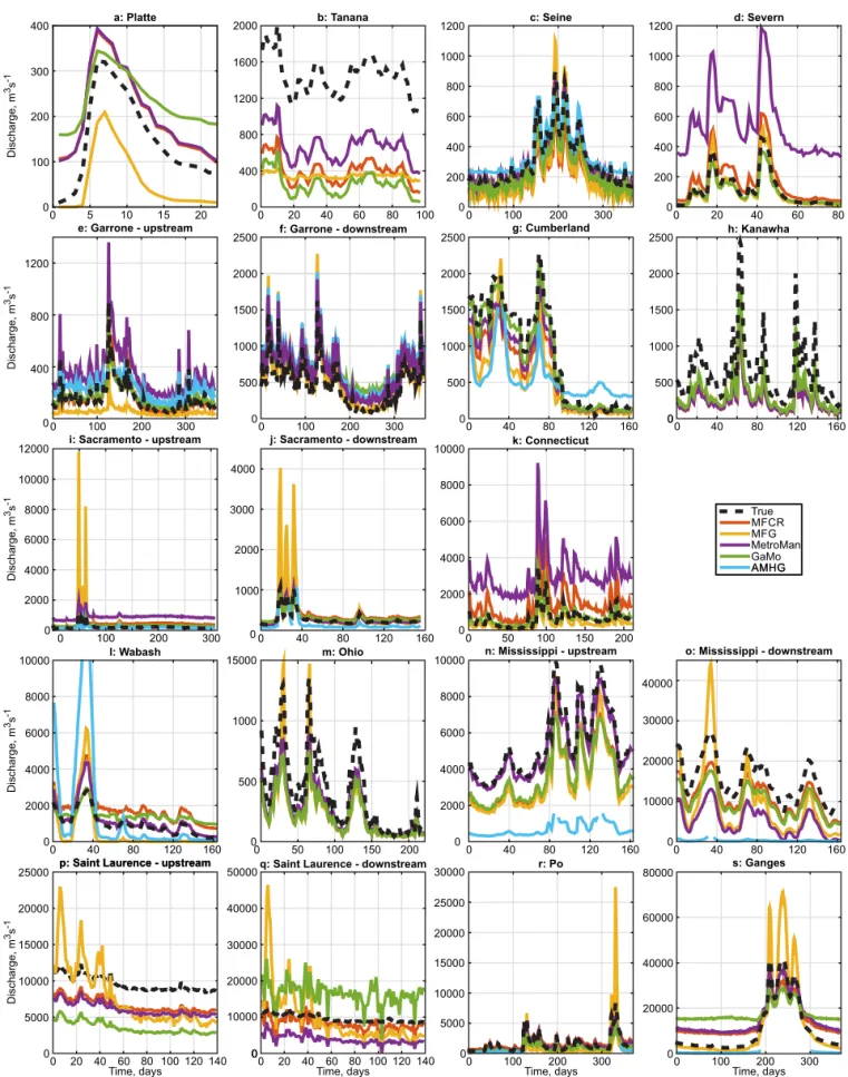
Time series of river discharge estimated on each river are shown in Figure 5. Table 5 summarizes the per-formance of each of the six algorithms for every river according to each of the three metrics described in section 2. RRMSE is perhaps the most important assessment metric, as this error determines how well each algorithm performed across the entire time series of observations. Thus, RRMSE can be considered the cen-tral ‘‘accuracy’’ metric in this study, and is directly comparable across scales for the 19 rivers here. We use an RRMSE of 35% as a threshold for algorithm performance; this number is admittedly arbitrary, but was cho-sen to improve upon the accuracy values cited for global models (40%) in the introduction. RRMSE values ranged from 5% to greater than 100% across all rivers and all algorithms. Viewed collectively, at least one algorithm had an RRMSE less than 35% for 14/19 rivers, and the grand median RRMSE (across all six algo-rithms and 19 rivers) was 55%; note that some of the algoalgo-rithms yielded highly biased results, such that the mean across all rivers and algorithms is 87%. Five of the six algorithms had the best estimation RRMSE for at least one river, with MetroMan having the best performance for eight rivers, MFCR performing best for four rivers, GaMO and MFG performing best for three rivers each, and AMHG giving the best estimate on one river. Interestingly, the ensemble median algorithm did not give the best result on any river, despite selecting the median flow value of the other five algorithms at every point in time. At least one algorithm had an RRMSE greater than 100% in 9/19 rivers. Figure 6 summarizes and compares the performance of each algorithm.
Braided rivers were particularly difficult to estimate, as none of the Ganges, Platte, or Tanana Rivers had an algorithm register an RRMSE less than 35%. In addition, the Ganges and Platte Rivers each had three algo-rithms record an RRMSE greater than 100%. This mirrors the findings ofGleason et al. [2014], and further confirms the difficulty of estimating discharge via remote sensing in braided rivers. Removing these braided rivers from consideration results in 14/16 rivers having at least one discharge RRMSE less than 35%.
ability is especially impacted by low-biased prior estimates of mean streamflow. Thus, MetroMan estimation accuracy is expected to be better for a prior with a positive bias than for a negative bias. AMHG was not run for the Kanawha, as only 1.5% of cross sections passed the low-b filter. This combination of a poor, negative bias in the prior, and the inability to use AMHG, highlights a weakness in the overall set of algorithms.
In addition to overall performance, the stability of the algorithms across rivers is of critical importance to the SWOT mission and to discharge inversion more generally. Stability is assessed by SDRR and its relation-ship to the MRR per river, and also by summarizing RRMSE across rivers. For all 19 rivers, at least one algo-rithm had an SDRR less than 31%. We had hypothesized that the ensemble median would be the most stable algorithm, and indeed it had an SDRR less than 30% in 13 cases, tying for best SDRR performance with GaMo, which also had 13 rivers less than 30% SDRR. For the ensemble median algorithm, the median SDRR value across the 16 nonbraided rivers was 12.5%. Considering the summary metrics in Table 5, MFG and MFCR, two approaches that require an a priori flow, performed quite well; one of these two had the lowest SDRR for 8/19 rivers.
Overall, most algorithms had an even distribution of negative and positive residual bias across rivers, as indicated by MRR. However, AMHG had a positive bias for 7/11 rivers (note that eight rivers were considered unsuitable for AMHG estimation as they were either braided or did not pass the width variability filters described in section 3.1), and MFG had a strong negative bias, overestimating flow in 16/19 cases. The dif-ference between the WBM mean annual flow estimate and the mean true flow for each river (see Table 2) can be compared with the MRR results in Table 5. Across all 19 rivers, the median WBM bias is237.9%. Five of the six algorithms (AMHG, GaMo, MetroMan, MFCR, and the median) have a median MRR that is less than WBM.
Figure 5 shows that certain rivers were more easily estimated than others. In particular, all algorithms had an RRMSE less than 45% for the Seine, confirming it as the most easily estimated river. In addition, we might expect that the MetroMan and GaMo algorithms would perform similarly from river to river, as each is based on solving for unknown parameters in Manning’s equation. This is confirmed in our results, as these two algorithms both had an RRMSE less than 35% for the Downstream Sacramento, Seine, Po, Upstream Missis-sippi, and Ohio Rivers (Figure 6). Also, while estimations from the Cumberland and Kanawha rivers were poorer than other rivers, all algorithms but AMHG had very similar estimation accuracies in these rivers. Beyond predictably poor performance in braided rivers, there are no apparent trends in algorithm perform-ance based on river size, flow range, WSE variability, latitude, or hydraulic regime. A possible exception here
Table 5.Summary of Discharge Estimation Output According to Three Metricsa
RRMSE (%) MRR (%) SDRR (%)
River Name AMHG GaMo MetroMan MFG MFCR Median AMHG GaMo MetroMan MFG MFCR Median AMHG GaMo MetroMan MFG MFCR Median
Connecticut n/a 29.2 696.5 43.6 161.3 93.9 n/a 19.7 571.5 243.0 149.7 84.7 n/a 21.6 399.1 6.9 60.1 40.6 Cumberland 175.6 47.9 44.6 50.6 45.5 47.2 246.5 22.7 214.5 242.6 227.3 218.8 169.9 48.0 42.3 27.5 36.5 43.5 Garrone (DS) 80.5 128.8 70.4 16.3 87.6 86.8 264.6 95.4 59.2 13.9 73.6 71.7 48.1 86.7 38.2 8.7 47.5 49.0 Mississippi (DS) 98.3 35.7 72.8 58.8 28.4 59.2 98.3 235.6 271.7 250.9 228.2 257.1 0.4 2.9 12.5 29.5 3.3 15.8 Sacramento (DS) 58.6 26.8 4.8 50.4 42.0 6.0 55.3 22.5 22.1 7.0 41.1 0.1 19.6 14.6 4.3 50.0 8.7 6.0 St. Lawrence (DS) n/a 77.4 61.3 63.6 23.4 61.3 n/a 71.2 260.5 25.8 217.1 260.5 n/a 30.5 9.7 63.6 16.0 9.7
Ganges 93.2 279.8 152.8 36.8 133.2 133.3 93.2 214.2 122.9 220.1 101.8 103.8 1.2 180.2 91.0 30.8 86.0 83.7 Kanawha n/a 46.7 59.7 51.5 60.4 55.5 n/a 246.4 259.6 251.3 260.2 255.4 n/a 4.9 4.0 4.5 4.1 3.7
Ohio n/a 42.7 33.5 41.4 42.8 41.8 n/a 241.5 231.5 239.3 241.9 240.6 n/a 9.9 11.5 13.2 8.8 10.0 Platte n/a 347.7 215.9 77.0 223.0 219.3 n/a 174.3 106.0 274.5 106.0 104.7 n/a 307.9 192.6 20.1 200.8 197.3
Po 66.4 29.8 13.9 73.6 43.4 28.1 66.3 229.6 3.3 266.1 35.7 228.1 3.4 3.9 13.5 32.3 24.6 1.8
Seine 33.9 22.5 9.1 45.3 42.1 22.2 227.4 221.7 22.6 241.7 241.7 221.2 19.9 5.9 8.8 17.7 5.8 6.6 Severn n/a 17.6 1028.7 22.5 89.6 48.9 n/a 24.1 799.3 217.9 75.1 37.8 n/a 17.3 651.6 13.7 49.1 31.2 Tanana n/a 83.6 54.5 76.0 73.6 73.0 n/a 283.4 254.3 276.0 273.4 272.9 n/a 5.8 4.7 1.7 5.3 4.2 Garrone (US) 86.2 28.9 153.1 63.2 10.4 29.5 280.9 22.4 145.3 262.7 1.4 24.8 29.7 18.4 48.2 7.9 10.3 15.9 Mississippi (US) 88.2 35.1 5.9 41.4 36.3 36.4 88.2 234.9 25.8 240.4 235.8 235.9 2.1 3.8 1.0 8.8 5.9 6.1 Sacramento (US) 11.0 69.1 383.7 87.4 128.7 69.7 1.2 64.7 374.7 41.6 125.0 67.1 10.9 24.5 82.9 77.0 30.4 18.8 St. Lawrence (US) n/a 63.6 36.7 39.9 30.8 37.9 n/a 263.4 236.6 222.6 230.7 237.4 n/a 4.7 3.0 32.9 2.9 6.2 Wabash 98.4 146.1 26.2 92.2 134.9 27.9 28.0 99.1 22.5 274.4 117.6 23.5 94.6 107.7 13.5 54.7 66.4 15.0 Median 86.2 46.7 59.7 50.6 45.5 48.9 28.0 22.7 22.1 241.7 1.4 218.8 19.6 17.3 13.5 20.1 16.0 15.0
Mean 80.9 82.1 164.4 54.3 75.7 62.0 19.2 22.1 98.2 235.1 24.8 4.8 36.4 47.3 85.9 26.4 35.4 29.7
Standard Deviation 40.0 87.0 261.2 20.0 54.9 46.9 63.2 77.9 228.5 31.4 69.7 57.1 49.9 75.8 162.6 20.9 46.0 44.4
a
is the Platte, for which algorithms performed quite poorly, and was the only kinematic river analyzed. Note that kinematic rivers show no time variability in water surface slope, which for some algorithms similar to those tested here leads to poor performance [Durand et al., 2010]. However, since the Platte is also braided, and other kinematic rivers were not included, no firm conclusion can be drawn; further work is required. Given that the data here are models of rivers forced with imposed flows, comparison of algorithm perform-ance against morphology is inappropriate. However,Gleason et al. [2014] found no apparent trends in esti-mation accuracy for the AMHG algorithm based on river morphology in their study, so the lack of clear physical controls on discharge estimation accuracy is perhaps unsurprising.
5. Discussion
This discharge algorithm intercomparison has highlighted both successes and failures of algorithms thus far. First, we have seen that there is always an algorithm that estimates discharge to within 35% or less RRMSE for 14/16 nonbraided rivers. Second, bias has proven itself to be a significant component of these errors; the median algorithm had an SDRR less than 30% for 13/19 rivers, but an RRMSE less than 30% for only 5/19 rivers. Third, we have seen that one single algorithm has not emerged as the ideal approach. Instead, we hypothesize that the community will likely require moving forward with multiple approaches. These results can be used to map future algorithm developments within the SWOT community.
Simply put, the addition of more a priori data and site-specific assumptions should make each of the algo-rithms more effective. However, this study was truly blind. Thus, in all cases, there was information we knew about certain rivers that we purposefully did not include in our algorithms: all methods received the same data and were forced to make the same blind assumptions. Some prior estimate of roughness, AHG, dis-charge, or some other variable is available for every measured or modeled river on the planet. Leveraging these data should improve the performance of the methods here, as will using these methods in conjunc-tion with hydrologic models in assimilaconjunc-tion schemes, which is the likely way forward for using SWOT to esti-mate global river discharge.
The variable nature of algorithm performance in this study confirms the difficulty of the problem and the value of such a large-scale comparison. Each of the AMHG, GaMo, and MetroMan algorithms performed worse than their previously published accuracies in some cases, althoughGleason et al. [2014] also found varied performance for the AMHG algorithm in their study of 34 rivers. These mixed results occur despite the fact that inputs to the algorithms were ‘‘perfect,’’ i.e., not degraded to match expected temporal
sampling and observation error likely from SWOT.Yoon et al. [2016] found that MetroMan accuracy was not significantly affected by using SWOT temporal sampling and expected measurement errors on the Sacra-mento River as compared with daily sampling, but this result will likely vary among algorithms and rivers. When faced with real-world data, these algorithms will behave differently, and likely worse, than they have here if algorithms are not improved or ancillary data as described above are not included.
Our results strongly point to the need for algorithm synergy when conceiving of a SWOT discharge product that will be viable for all of the world’s rivers. We have tested the easiest likely approach for this synergy (the ensemble median), but each of these algorithms should be able to inform and constrain one another. For example, we may find that some algorithms tend to perform poorly for certain kinds of rivers, and in these cases, we ought to exclude those algorithms from the ensemble. As another example, it may be bene-ficial to create hybrid approaches built by combining components of the various algorithms. For example, the variablenof MFG could be combined with MetroMan or GaMo. Exploring these kinds of synergy should be a key goal of future algorithm development, together with identification of the best ancillary data for use with these methods.
It is critical to begin to be able to predict algorithm performance based on river characteristics. Perhaps surpris-ingly, the hydraulic regime analysis (Froude and kinematic wave numbers shown in Figure 2) did not correlate with algorithm performance, except that the one truly kinematic river (the Platte) performed quite poorly. We continue to explore this by discussing several of the cases included in the test cases: floodplain flow, low-head dams, and multiple channels. It had been hypothesized prior to this algorithm intercomparison that perform-ance would suffer during floodplain flow. An interesting case in this regard is the Po River. Figure 3 clearly shows out-of-bank flows: some reaches increase their width by an order of magnitude during the high flow event following day 300 of the simulation. The MFG algorithm is formulated with the assumption of in-bank flow, and overestimates flow by a large margin during this period; this leads to an underprediction of flow dur-ing the low-flow periods and an overall MRR of266.1%, and an RRMSE of 73.6%. However, the GaMo and Met-roMan algorithms perform well, with RRMSE of 29.8% and 13.9%, respectively. Thus, even the simple Manning formulations appear in-and-of-themselves to be adequate even in the presence of significant floodplain flow. This is in spite of the fact that the calibrated hydraulic models used to generate the synthetic observations in this study typically used different values ofnin the floodplain versus the channel, a fact not accounted for in the discharge algorithms. As a caveat to this point, it should be noted that the Po River model is built in 1-D; thus, we can really only conclude that 1-D floodplain flow is resolved by these algorithms.
Performance in the presence of low-head dams and human management was an open question prior to this study. Significant dams are present on the Ohio River, leading to quite low slopes, as shown in Figure 4. However, the MetroMan algorithm performs adequately on the Ohio, with RRMSE533.5%, and SDRR511.5%. Manning’s equation captured the friction losses, even in this case with low slopes, and signif-icant backwater profiles. Performance in the case of multiple channels was also expected to degrade per-formance. The Seine is an example of a multichannel river; throughout the domain utilized here, the river is often two channels. The simplest solution of merging the top widths and averaging the water surface heights [Schubert et al., 2015]) led to adequate performance, here: AMHG, GaMo, and MetroMan had RRMSE of 33.9%, 22.5%, and 9.1%, respectively. Thus, the presence of multiple channels is not necessarily a cause of a great deal of algorithm performance degradation.
Finally, one source of error not considered or evaluated here is error in the hydraulic models themselves. As each model is comprised of approximate hydraulic solutions imposed on in situ data of varying quality at varying spatial sampling and with simplified physics compared to real-world flows, it is quite likely, indeed almost certain, that reported widths and WSE values corresponding to reported discharges contain some error. How this error contributes to discharge estimation will vary by algorithm and by river, and assessing this effect on our estimations is well outside our purposes here. However, to the extent that the flow laws as implemented in the algorithm represent reality (such as with the empirical components of MFG), this effect should contribute little to discharge algorithm error.
5.1. Algorithm-Specific Discussion
5.1.1. At-Many-Stations Hydraulic Geometry
here. Previously, the method had only been tested with a maximum of 20 observations, and the increase to yearly or longer periods of observations caused significant issues with both AHG and AMHG. This increased number of observations also rendered the previous remotely sensed proxy for AMHG [Gleason and Smith, 2014] ineffective at adequately characterizing AMHG, as it is mathematically constrained to a value of 0.5 when there are order-of-magnitude changes in observed widths, which occurred in numerous study rivers. An incorrect AMHG proxy gives an incorrect relationship between AHG parameters, and therefore inverted AHG curves are constrained to a hydraulic space outside observed values. In addition, the minimum and maximum imposed flows in the AMHG algorithm were developed and tested on rivers other than those here (Gleason and Smith[2014] give ‘‘global’’ values ofQmin5minimum observed width30.5 m depth3 0.1 m/s velocity,Qmax5maximum observed width310 m depth35 m/s velocity). As before, using river-specific estimates of maximum and minimum depth and velocity will improve the AMHG method.
There are also hydrologic and geomorphological reasons why more observations lead to poorer AMHG per-formance. For example,Bonnema et al. [2016] show that for the Ganges River, AMHG exhibits a sharp improvement in accuracy when wet and dry seasons are estimated separately, whileGleason and Hamdan
[2015] show the same result for the Ganges (using different data fromBonnema et al. [2016]), noting a reduction from 56% to 28% RRMSE when considering dry-season flows only. This is because these wet and dry flows (or flood and nonflood regime for temperate rivers) exhibit different AHG behavior and have much different time meanwandQvalues, leading to a situation where discharge cannot be inverted [ Glea-son and Wang, 2015]. Additionally, when flows vary widely, AHG breaks down and must be represented with multiple power laws: one for each distinct channel geometry. Thus, it is recommended that AMHG be performed in a stepwise manner when many observations are available, as binning observations into those with similar magnitude widths should assure a single AHG curve per bin. As with all other algorithms, including these kinds of river-specific constraints will improve AMHG performance.
5.1.2. Garambois and Monier
The GaMo algorithm relied uponQMFCR(which in turn relied upon the WBM mean annual flow estimate) for
defining a first guess and minimum and maximum bounds for discharge. First guess and identification bounds are also defined forngiven usual values found in the literature [e.g.,Chow, 1959], and for low flow cross-sectional area from observed cross-section variations. Presumably, it is because of the use of these bounds that some of the very large RRMSE values observed with MetroMan are not observed with GaMo (compare Table 5), even though they are based on similar hydraulic flow laws. Note too, that despite relying onQMFCR, the GaMo algorithm resulted in better or comparable performances than MFCR for 16/19 rivers
(Table 5). This suggests that the GaMo approach can take some advantage of the hydraulic information from SWOT-like data to constrain river discharge estimation.
Future improvements to GaMo could involve adding additional constraining equations, or adding additional prior information, for example, to reduce the optimization zone in hydraulic parameter space. If discharge was supposed constant in space, the number of unknowns isNR3NP 11 and there are stillNR3NP
equa-tions, making the inverse problem more tractable [Garambois and Monnier, 2015]. This approach could be of interest for (large) rivers with small changes in flow between several reaches.Garambois and Monnier
[2015] also derived a robust and accurate inference method in the case that one in situ water depth mea-surement is available. Indeed, in this case, an explicit expression for the channel bed elevation is available as a function of the water surface slope and width, independent ofn. Next, given this channel bed eleva-tion, an approach similar to GaMo allows accurate computation of the inflow discharge.
5.1.3. Metropolis Manning
in future work, and could in principle be addressed by running several MCMC chains with different mean values.
An additional drawback of MetroMan (and indeed MFCR and GaMo, as well) is that it assumes thatn(or AHG in AMHG) does not change in time, i.e., with flow depth. Thus, any changes in bed or bank material, increases in debris, or reorganization of channel geometry will lead to suboptimal discharge estimation. This decision was originally made in algorithm formulation in order to limit the number of unknowns, but it agrees with the hydraulic models in this study. In most of these models,ndoes not vary in time at each cross section, except for marginal changes during out of bank flow. Therefore, this assumption is secure for these model data where debris and changes in substrate are generally not considered, but less secure for future observational data.
An additional drawback is that MetroMan invokes Manning’s equation at a river reach, not at a cross section. It is possible that Manning’s equation does not hold for reaches, even when using the true reach-averaged roughness coefficient, and even if Manning’s equation holds at each cross section. To analyze this, we esti-mated the ‘‘effective’’ reach average roughness coefficient for each river by calculating it at each time step from reach-average hydraulic quantities:
~
n5Q21A5=3W22=3S1=2 (8)
In Figure 7 (left), the effective roughness~nis compared to the reach average roughness coefficientn; the former is calculated from (8), while the latter is calculated as the average value of the roughness coefficient across all cross sections in a given reach. As flow decreases,~nincreases dramatically, whilenremains con-stant. Analysis of this phenomenon revealed this behavior was due to the increase at low flow of within-reach spatial variability of the cross-sectional area, width, and slope, combined with the nonlinear nature of Manning’s equation. While it is tempting to analyze this in terms of fluvial geomorphology or the physics of open channel flow, this finding is completely mathematical:n~diverges from n due to averaging of within-reach spatial variability.
Figure 7 (right) shows that the more~ndiverges fromn, the worse MetroMan’s bias. Here the divergence of
~
n from n is characterized by a factorj5ðn=n~Þ 21. Therefore,j50 means that there is no within-reach hydraulic variability asn5~n, and the more negative thej, the more variability there is (note that j<0, since~n>n). Of particular interest is the situation described above at low flow, wherejbecomes more and more negative as~nincreases but n stays constant. Figure 7 plots the minimumjfor each river versus Met-roMan MRR, and for minimumjvalues less than20.5, MetroMan MRR often becomes very large. Thus, the more within-reach variability of stream hydraulics, the worse MetroMan’s performance. Future work must consider how to include time-varyingnin MetroMan, and presumably other algorithms; work to incorporate the time-varyingnfrom MFG into MetroMan framework is ongoing.
It would be reasonable to assume that the significant increase in~nat low flow would impact GaMo in the same way that it impacts MetroMan, as both use reach-averaged quantities, require nto be temporally invariant, and solve for A0 andnby requiring continuity among reaches. However, the GaMo discharge
results do not diverge for high values ofj. The reason for this is presumably because GaMo specifies rela-tively restrictive minimum and maximum values of discharge, while MetroMan invokes prior information utilizing a cost function. Because MetroMan assumed a relatively high uncertainty in the prior mean annual flow estimate, and very precise observations with no allowance for error in Manning’s equation itself, unre-alistic discharge estimates were produced in the cases with large variations inn. GaMo did not allow these unrealistic discharge estimates because it was limited to the range of discharge estimated by MFCR.
5.1.4. Mean Flow and Geomorphology
Due to the empirical determination of some parameters, this method is not expected to work well for braided rivers and tidal reaches, where the controls on the flow resistance (and thus Manningn) are very different than in single or slightly anastomosed channels. Additionally, the accuracy and applicability of the algorithm is expected to be limited by the need for the prior mean annual flow. By design, the MRR for the MFG algorithm is highly correlated (R250.86) with the WBM bias. For example, the WBM mean annual flow
estimate for the upstream Garonne underestimates the flow during the experiment by 65%, while the MFG MRR is263%. One additional limitation of MFG is that it is not expected to work well for floodplains, since out-of-bank flow was not used in deriving the relations. Indeed, MFG performs relatively poorly for the Po (RRMSE573.6%) due in part to significant overestimation of high flows (see Figure 5).
For the application of this algorithm, future efforts should focus on improving the empirical aspects of the method with additional site-specific information, and over time with more observations. This is particularly important in reaches that are braided or tidally influenced where unique more specific relations may be developed. It is also possible that other geomorphologic information about the channel planform (including meander length, sinuosity, and channel type) can inform the estimation of Manning n, as indicated by Bjer-klie[2007]. Additionally, the Manning equation, which forms the physical basis for this method, also forms the basis for the MetroMan, GaMo, and MFCR algorithms and as such the three independent methods should eventually converge to similar values provided the assumptions and relations used in both corrobo-rate each other. For example, the optimization scheme used in MetroMan or GaMo to optimizeA0andn
could also be used to optimize the value ofB, and the value ofnin MetroMan and GaMo could be esti-mated a priori from various empirical relations and channel morphology.
5.1.5. Mean Flow and Constant Roughness
The philosophy of the MFCR algorithm was to preserve the mean flow estimated by WBM, while simply assuming a defaultnvalue of 0.03. Any error in WBM flow should propagate directly in error in the MFCR algorithm. However, there are cases where the WBM estimate is too low but the MFCR is biased too high, e.g., in the case of the Connecticut River. The mean HEC-RAS flow for the Connecticut in this study (June– December, 2011) was 1208 m3/s, whereas the WBM estimated flow for this time was 394.1 m3/s. Therefore,
constraints of a roughness coefficient of 0.03 and a nonnegative flow area, flow is estimated as far higher than specified mean annual flow.
Intriguingly, there is a slight dependency of the overall MFCR bias on the average Froude number of each river; lower Froude numbers had more tendency to have a low bias, and vice versa; the mean Froude num-ber explains approximately 53% of the variance in the bias of the median estimate. In general, larger higher Strahler order streams have lower slope and lower Froude numbers, and these rivers generally had more negative bias. Presumably, this has to do with the WBM simulations used to estimate the MFCR mean annual flow.
These results highlight interesting conclusions about simple ‘‘prior’’ type flow estimations that point to the need for the more complex algorithms discussed before. First, the low value of mean flow from WBM did not agree with the large observed cross-sectional area changes, underscoring the dangers of relying on prior conditions to estimate discharge. Second, discharge estimation via the prior resulted in the opposite bias as WBM, pointing to how critical it is to develop a better understanding of hown~behaves. Finally, our results suggest that using only a few cross sections cannot be used to represent a reach average.
5.1.6. Ensemble Median
Thus far, it is difficult to predict which algorithm will perform best on each river; thus, the ensemble median is a highly attractive option. It is somewhat unexpected that the ensemble median is not the top performer on any of the 19 rivers, on the basis of RRMSE. However, it is quite encouraging that overall, the median is the least biased of any of the six estimates; the ensemble median algorithm has a mean MRR across the 19 rivers of just 4.8%. However, the standard deviation of the ensemble median algorithm’s MRR is 57.1%, sug-gesting that variation in algorithm performance at each river was varied enough to render the ensemble median unreliable. It is expected that this issue will be addressed in the future, as the described major issues with reach averaging are explored, and prior and/or river-specific information is incorporated in discharge estimation. As individual algorithms improve, so too will their ensemble products.
6. Conclusion
We are encouraged by the current state of SWOT discharge algorithms: 14/16 nonbraided rivers had an algorithm estimate discharge within 35% RRMSE of true flow. These results include rivers with complex real world hydraulics like 1-D floodplain flow, low-head dams, and simple multichannel rivers. Some of these complex hydraulics and geomorphologies can have a strong effect on the methods discussed here: extreme flood events, braided rivers, and two-stage AHG all lead to decreased performance. Discharge algorithms must be improved to handle these cases, and methods to quantitatively predict algorithm performance based on river morphology must be developed. Moreover, the experiments conducted in this study used idealized synthetic daily observations with minimal noise; future studies designed to test SWOT’s ability to estimate discharge need to use SWOT-like temporal sampling and error characteristics and work with observed field and airborne data sets when possible. Our results from this experiment also indicate that algorithm improvement is needed if a robust, global discharge product is to be delivered from SWOT, as no single algorithm or their ensemble median performed with consistently accurate results. The MetroMan algorithm comes closest, as it was the most accurate algorithm in 9/16 nonbraided rivers, but even this algorithm is subject to very large discharge errors in other cases. We conclude that our restrictive experi-ment design, where no ancillary data or river-specific assumptions were allowed is a likely cause of many of the poor results, substantiated by previous studies using each of the AMHG, GaMo, and MetroMan algo-rithms. Future work seeking to estimate discharge from remotely sensed platforms should include as much ancillary data as are available, and also seek to develop multialgorithm synergy to improve stability and accuracy of derived discharge retrievals.
References
Adams, T., S. Chen, R. Davis, T. Schade, and D. Lee (2010),The Ohio River Community HEC-RAS Model, pp. 1512–1523, Am. Soc. of Civ. Eng., Reston, Va.
Andreadis, K. M., E. A. Clark, D. P. Lettenmaier, and D. E. Alsdorf (2007), Prospects for river discharge and depth estimation through assimila-tion of swath-altimetry into a raster-based hydrodynamics model,Geophys. Res. Lett.,34(10), L10403, doi:10.1029/2007GL029721.
Acknowledgments
Funding for this work was provided by NASA SWOT Science Definition Team grants NNX13AD96G and
NNX13AD88G, NASA Terrestrial Hydrology Program grant